Abstract
Coastal dunes are globally-distributed dynamic ecosystems that occur at the land-sea interface. They are sensitive to disturbance both from natural forces and anthropogenic stressors, and therefore require regular monitoring to track changes in their form and function ultimately informing management decisions. Existing techniques employing satellite or airborne data lack the temporal or spatial resolution to resolve fine-scale changes in these environments, both temporally and spatially whilst fine-scale in-situ monitoring (e.g., terrestrial laser scanning) can be costly and is therefore confined to relatively small areas. The rise of proximal sensing-based Structure-from-Motion Multi-View Stereo (SfM-MVS) photogrammetric techniques for land surface surveying offers an alternative, scale-appropriate method for spatially distributed surveying of dune systems. Here we present the results of an inter- and intra-annual experiment which utilised a low-cost and highly portable kite aerial photography (KAP) and SfM-MVS workflow to track sub-decimetre spatial scale changes in dune morphology over timescales of between 3 and 12 months. We also compare KAP and drone surveys undertaken at near-coincident times of the same dune system to test the KAP reproducibility. Using a Monte Carlo based change detection approach (Multiscale Model to Model Cloud Comparison (M3C2)) which quantifies and accounts for survey uncertainty, we show that the KAP-based survey technique, whilst exhibiting higher x, y, z uncertainties than the equivalent drone methodology, is capable of delivering data describing dune system topographical change. Significant change (according to M3C2); both positive (accretion) and negative (erosion) was detected across 3, 6 and 12 months timescales with the majority of change detected below 500 mm. Significant topographic changes as small as ~20 mm were detected between surveys. We demonstrate that portable, low-cost consumer-grade KAP survey techniques, which have been employed for decades for hobbyist aerial photography, can now deliver science-grade data, and we argue that kites are well-suited to coastal survey where winds and sediment might otherwise impede surveys by other proximal sensing platforms, such as drones.
Keywords:
coastal dunes; drone; KAP; kite; monitoring; structure-from-motion; change analysis; Photoscan; point cloud 1. Introduction
Sand dune ecosystems are globally distributed [1], covering approximately 34% of the world’s ice-free coastlines [2], and they form on many types of shores and under a variety of climatic conditions [3]. They deliver critical ecosystem services such as coastal protection [4] as well as providing environmental heterogeneity which promotes ecological diversity [5]. Other services include nutrient cycling, well-being and recreation, and mineral extraction [6]. Whilst these services are beneficial to human populations at the coast and beyond, coastal sand dune environments face pressures. The threats to sandy beach ecosystems and their associated dunes are wide ranging from local to global in scale [7]. Dune systems worldwide are under threat from increased storm damage and human interference such as pollution, and human disturbance (e.g., off-road vehicles and trampling [8,9]). There is a pressing need to monitor these sensitive environments in order to inform management decisions for preserving their integrity and averting irreversible damage [10].
A wide range of scientific work has used field, laboratory and spatial modelling approaches to understand the fine-scale dynamics of sand dune systems, and to identify which physical processes shape them (e.g., 2D profiles to understand how sediment budgets influence foredune structure [11]). Numerical modelling approaches incorporating wave dynamics have also been utilised to understand the response of coastal dunes to environmental change such as storm events and hurricanes [12]. Monitoring of dune condition is critical to ensure the provision of the services they provide, to complement understanding of the natural processes shaping coastal dunes. The task of monitoring can be greatly aided by data from remote sensing systems. To date, a variety of both remote and proximal sensing techniques have been used to answer questions about dune morphology, dynamics and change, and for the management of dune systems. For example, terrestrial laser scanning (TLS) has proven useful for quantifying coastal dune morphology [13], and repeat TLS has been used successfully to monitor the evolution of erosion features such as dune blowouts [14]. TLS has also been deployed to track erosion and predict overtopping of anthropogenic berms on the coast [15]. Despite the very high precision (<10 mm) and fine spatial resolution (~7 mm at 50 m range; [16]) data that TLS systems can provide, the equipment is expensive, complex and time consuming to operate [17]. The spatial extent over which it can be employed is also limited as positioning of the equipment has to be carefully considered to avoid gaps in the data collected, and the most beneficial positions for the equipment may not always be accessible [16]. From commercial satellite systems, relatively fine spatial (0.61 m panchromatic) resolution data such as those delivered by Quickbird, we argue, are poorly suited for cost-effective monitoring of dynamic systems such as those found in coastal environments. This is because dune systems are highly dynamic and repeat surveys are often required to gain understanding of the processes at work in the coastal zone, necessitating the purchase of multiple data sets, which can become very costly, sometimes prohibitively so for long-term monitoring programs [18,19]. Furthermore, despite their fine spatial resolution, issues such as mixed pixels can still arise in dune environments due to a high degree of habitat heterogeneity and mixtures of vegetation and sand [20]. Alternatives to Quickbird include data provided by the Landsat and Sentinel 2 sensors for which global median revisit times are approximately 3 days [21]. However, their coarser spatial resolution (>10 m) are unsuitable for monitoring the heterogenous environments found at the land-sea boundary, where the mixing of terrestrial and marine realms again can give rise to mixed pixels, ultimately reducing the success of delineating key landcover types. Aside from satellite platforms, data collected during airborne campaigns both with Light Detection and Ranging (LiDAR) and optical sensors have been utilised for coastal monitoring [22]. For example, LiDAR data have been used to aid the estimation of shoreline slope and position over hundreds of kilometres of coastline [23], to conduct shoreline change analysis on centennial and intra-decadal scales [24], and to complement ground based vegetation surveys to identify major habitat types to improve understanding of the relationship between dune structure and plant species occurrence [25]. In combination with airborne multispectral data, LiDAR data have shown promise for classifying coastal habitats [26]. However, high costs of piloted aerial surveys prohibit the commissioning of airborne campaigns for regular monitoring [27], and are not feasible in countries where such survey resources are unavailable.
Proximal sensing from low-cost lightweight drone and kite platforms has seen a recent rapid uptake within the geosciences and biosciences for environmental monitoring purposes [28,29]. Reasons for this include the low cost of the technology, ease of use, user-dictated surveys both in time and space and the ability to customise the payloads (e.g., sensors) that are attached to the platforms. In parallel, the increased availability of high performance computers and development of photogrammetry software means that Structure-from-Motion Multi-View Stereo (hereafter: SfM-MVS) techniques are now easily employable using images collected from consumer grade cameras [17,30]. SfM-MVS has been used to study geomorphological features such as glacially sculpted ridges [17], estimate biomass in tropical forest environments [31] and create digital surface models of coastal dune environments [32]. Fine spatial resolution data (typically sub-centimetre) have been used to quantify the heterogeneity of seagrass meadows [33], conduct coastal vulnerability assessments [34], map mangroves [35] and quantify changes in vegetation within dune ecosystems [36,37]. Although these prior experiments have demonstrated the opportunities for this new approach to be adopted widely in coastal environments, drone operations specifically are not without their risks in these settings. First, coastal environments have a tendency to be windy and this makes both operating drones and capturing high quality data here more challenging [38]. Second, the presence of loose sediment such as sand particles poses a risk to mechanical drone parts such as motors, and parts of the on-board payloads (e.g., camera lenses). One alternative that mitigates some of these issues is kite aerial photography (KAP). The natural fuel source of the wind in coastal systems makes KAP a cost-effective and accessible method with which to collect proximal sensing data [29]. Kites have been used for data capture in ecological studies, e.g., to monitor penguin population sizes [39], for geomorphological applications such as the catchment scale gully detection [40] and intertidal landscape mapping [41], but there are no similar studies documenting the use of kites for sand-dune mapping and topographic change mapping over time.
The self-service nature of proximal sensing from KAP platforms facilitates data capture at high temporal resolution (i.e., possibility of multiple surveys in one day) and fine spatial resolution. Alongside, the emergence of high performance and affordable computing power allows for the analysis of SfM-MVS data outputs. Analysing the changes in the structure of features represented in such data (e.g., point clouds), whilst also taking account of data uncertainty, can now be achieved with the Multiscale Model to Model Cloud Comparison (M3C2) technique [42]. This method improves on the difference of DEM (DoD) technique by incorporating 95% confidence intervals into change detection between the points in two clouds, also allowing for the detection of very small changes and indicating whether they are statistically significant. Building on this, the M3C2-Precision Mapping (M3C2-PM) technique has been developed; incorporating Monte Carlo creation of multiple point clouds to derive precision estimates for each point in the cloud [43]. This type of analysis can readily be applied to the outputs of SfM-MVS workflows. To our knowledge, the combination of KAP and SfM-MVS techniques involving multi-temporal surveys has not been undertaken to date using M3C2-PM methods. Neither has the method been demonstrated robustly for coastal monitoring over time. We address the following research questions to explore these knowledge gaps:
- (1)
- How do data from a KAP system processed with SfM-MVS methodology compare to similar data captured from a more stable drone system for sand-dune morphological assessment at a single point in time? Given existing work that allows robust estimates of spatial uncertainty to be obtained for SfM-MVS derived point clouds (e.g., M3C2-PM), we apply such methods to the data produced from the drone survey and a single KAP survey to understand differences in the data produced.
- (2)
- To what extent can a KAP + SfM-MVS methodology capture fine spatial scale (sub-decimetre) changes in sand-dune morphology over time? Applying M3C2-PM analysis techniques, we aim to determine the extent to which significant changes can be detected in sand-dune morphology from multi-temporal KAP-SfM-MVS data products, focussing on three-, six- (intra-annual) and twelve-month (inter-annual) timescales.
- (3)
- Employing such methods, how do beach, dune fronts/foredunes, and footpaths change over time?
2. Materials and Methods
2.1. Study System
The study system used for this proof-of-concept work was located within St Gothian Sands Local Nature Reserve (50.226, −5.392) on the north coast of Cornwall in south-west England (Figure 1). A stretch of foredunes measuring approximately 180 m in length was selected for data collection. Although now protected, the site was exploited for sand extraction until 2005 [44]. It is now a popular recreational site with dog walkers, and other beach goers throughout the year. The predominant wind direction at the site is westerly followed closely by southerly winds (Figure 2).
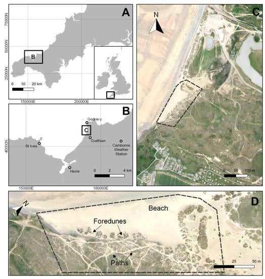
Figure 1.
(A) The location of St Ives bay and Gwithian Towans within the UK and Cornwall; (B) The location of St Gothian Sands Local Nature Reserve; (C) An aerial image (courtesy of Channel Coastal Observatory, https://www.channelcoast.org/) with the dune study system (area of interest) indicated by dashed line; (D) The study system annotated with features of interest.
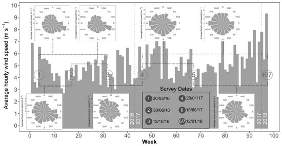
Figure 2.
Wind profile characterising the study system using weather data from Camborne weather station (located approximately 5 km east of St Gothian Sands nature reserve). Histogram displays average hourly wind speed (grouped by week) throughout the study period, and wind roses indicate average hourly wind speed and direction during the periods between pairs of the six KAP and drone surveys used in analysis (indicated by number labels). Weather data obtained from Met Office DataPoint Service (https://www.metoffice.gov.uk/datapoint; contains public sector information licensed under the Open Government Licence).
2.2. Data Capture
KAP was used to collect aerial images of the site. Two variants of the same kite were used, depending on weather conditions, but both were single line foil systems (HQ KAP Foil 1.6 m2 and HQ KAP Foil 5.0 m2) that are renowned for providing stable aerial platforms. The 5.0 m2 model was suitable for lower wind conditions (1.79–8.94 m s−1), whilst the 1.6 m2 model was suitable for higher wind conditions (3.13–13.86 m s−1), which were more typical at the site. A custom 3D printed picavet mount (created by author JPD: https://www.thingiverse.com/thing:1372969) was used to carry a ruggedized, waterproof and dustproof Canon D30 compact digital camera with a 5–20 mm focal length lens and 12.1 effective megapixel sensor (Figure S1). Picavet refers to a system of cords and/or pulleys designed to keep a platform stable. The camera also has an internal GPS sensor, recording positional information and storing it as metadata on each image captured. The Canon Hacking Development Kit (CHDK; [45]) was loaded onto the SD card inside the camera to allow for manual control of settings such as shutter speed, aperture, ISO and the time interval between consecutive image capture. The majority of surveys were conducted before 13.00 (GMT), but exact times varied depending on light availability and wind conditions at different times of year (Table 1). Wind conditions dictated the altitude of the kite, and sufficient line was deployed until the platform was deemed stable to commence surveying: Typically this was between 20 m and 40 m of line, but the angle between the kite and the ground varied during and between surveys due to temporally variant wind speeds, resulting in variations in spatial resolution both within and between surveys. The variation in sensor altitude was calculated as part of the SfM-MVS workflow. Six surveys were conducted between 30 March 2016 and 12 January 2018, to capture potential structural change at 3, 6 (intra-annual) and 12 months (inter-annual) periods (Table 1).

Table 1.
Details of each KAP and drone survey undertaken and associated wind conditions. Times (in GMT) are estimations based on the first and last photos that are deemed useable in the photogrammetry workflow. Wind data from Camborne weather station (located approximately 4.7 km ESE from the study system (Figure 1B)). Weather data obtained from Met Office DataPoint Service (https://www.metoffice.gov.uk/datapoint; contains public sector information licensed under the Open Government Licence).
To deliver an independent dataset for comparison to the KAP-SfM-MVS data, a single additional survey was undertaken using a 3DR Solo lightweight multirotor drone on the same date as survey 6 (Table 1) over a small sub-area of the dune study system, specifically to answer research question 1 (Figure S2). This type of drone has been previously used to collect high quality proximal sensing observations of coastal seagrass environments [33]. A short ~4-min flight with a fixed altitude of 40 m and speed of ~3 m s−1 was undertaken ~30 min after survey 6 (Table 1). Resulting data allowed for the direct comparison of point clouds constructed with images from the kite platform to those from the drone platform. The same sensor and setup (Cannon D30 with CHDK) was used with the multirotor drone as was used with the KAP methodology, with identical camera settings.
To provide independent ground control for spatial constraint of the SfM-MVS model [46], 14 black and white chequered 300 mm × 300 mm plastic ground control points (GCPs) were distributed across the area of interest (except for survey 1, where 14 were deployed but only 12 successfully measured due to technical issues with field equipment). A laminated card with a letter (a unique identifier, e.g., “A”) and a notice to ask beachgoers not to interfere with the target was placed alongside. The position of these GCPs was measured both with a handheld GPS device (Garmin GPSMap 64) and using a Leica GS-08 differential Global Navigation Satellite System (D-GNSS). The D-GNSS system uses a base and rover to deliver a differentially corrected geospatial location dataset with approximately 10 mm accuracy in x, y, z dimensions. Geospatial data collected with these two devices were recorded in the British National Grid projection (EPSG:27700). A cross was etched into on a concrete platform within the dunes, marking a single point to be used throughout the study period, as the base location for each repeat survey (easting = 158,199.7 m, northing = 41,825.74 m, altitude = 6.34 m). Ground-based photos were also taken of this point and its surroundings to aid in its relocation at the beginning of each survey. To minimise the distribution of error across the dataset, GCPs were placed in approximately the same positions according to their position from survey 1, using the handheld GPS as a guide to locate these positions during each revisit to the site. The data collection, processing and analysis workflow can be seen in Figure 3.
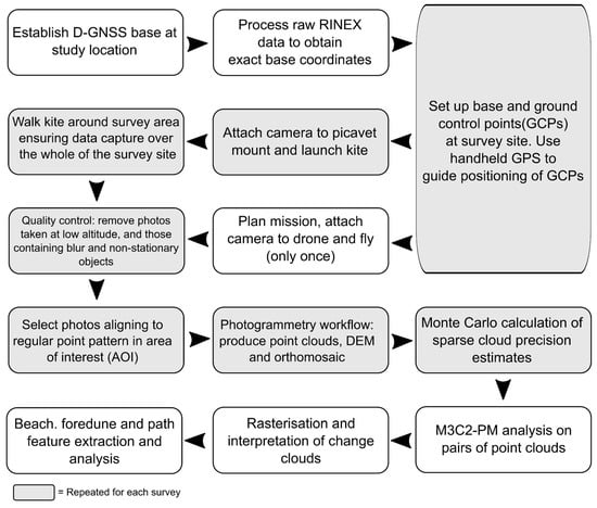
Figure 3.
Data collection, processing and analysis workflow for KAP and drone surveys.
Weather data were obtained from the Met Office DataPoint Service (https://www.metoffice.gov.uk/datapoint which provides public sector information licensed under the Open Government Licence). The nearest Met Office weather station to the study site with hourly recordings of weather conditions including wind speed and direction was Camborne in Cornwall (latitude: 50.218, longitude: −5.327), which is approximately 4.7 km ESE from the study system (Figure 1B). This data assisted in characterising the general wind conditions within the study system and between survey dates (Figure 2).
2.3. Data Processing
2.3.1. Sub-Setting Images
Images from each survey were manually filtered. First, those with visible blur, non-stationary objects (e.g., humans and dogs), and “low-altitude” images (e.g., captured during take-off and landing) were removed. A copy of all remaining images were loaded into Photoscan and a ‘low-quality’ alignment procedure conducted. This process estimates a camera position in the x, y and z dimensions for each image. These positions were then tagged to the metadata of each image using the freely available exiftool software package [47]. Given the level of processing required in the SfM-MVS workflow and the number of images collected during each survey, ~300 was chosen as a suitable number of images to include for photogrammetry processing. Using the spatstat package [48] in R 3.3.3 [49], a regular point pattern (n = 298, spacing between points ~7.70 m) was constructed within the bounds of the area of interest, and then a nearest neighbour procedure was conducted to find the closest image to each point. The nearest neighbour analysis was conducted iteratively, recording the identity of the image with the shortest Euclidean distance, removing the image and regular point from the selection and repeating. This resulted in a subset of 298 images for each survey. These subsets were then used as ‘raw data’ for the photogrammetric workflows (Figure 3).
2.3.2. Photogrammetry Workflow
Point clouds and associated elevation models and orthomosaics were built using Agisoft Photoscan (v 1.3) [50]. Processing reports for each build can be found in the supplementary information. Using the subset of 298 images from the sub-setting procedure as an index, the images containing metadata with positional information captured by the sensors internal GPS (original images) were assigned for the SfM-MVS workflow. Prior to processing, the latitude and longitude metadata values were converted from WGS84 (EPSG:4326) to British National Grid (EPSG:27700) format to match the co-ordinate system which was used for surveying ground control points with the D-GNSS. This conversion was undertaken in the statistical software R (version 3.3.3) [49], using the sp package [51] and image metadata were modified with exiftool [47]. Once initial alignment was undertaken, and a mesh constructed based on the sparse cloud, GCPs were located within the images and positional information from the D-GNSS attached. Further details on the full processing workflow in Photoscan can be found in the supplementary information.
2.4. Analysis
To investigate morphological change between surveys, a modified M3C2 approach which incorporates precision estimates for the point clouds was used [42,43]. This technique is well-suited to multi-temporal KAP topographic change estimation, where variation in data capture between surveys requires consideration within the analysis. Precision estimates for each point in the sparse clouds were calculated with Monte Carlo iterative processing in Photoscan, utilising pseudo-random offsets applied to the image observations and control measurements on each iteration. Full details can be found in the supplementary information of [43]. Given that the clouds varied in size between surveys, the number of iterations in the process varied (restricted by computer memory availability), with the estimated maximum possible number rounded down to the nearest 100 (Table S1). The estimates were then mapped (with a nearest neighbour approach) to the associated dense clouds and the M3C2-PM approach used to calculate changes in distance between pairs of clouds using the M3C2-PM plugin in Cloud Compare [43,52]. The M3C2 change detection was then conducted on the two clouds and their precision estimates, and a change cloud derived as a result for pairs of surveys. Within the change cloud, points that changed significantly in position were flagged to differentiate them from other points in the cloud. Change clouds were exported scaled down, reducing their density to approximately 0.5 m between points, so they could be analysed and rasterised for visualisation more effectively.
For the specific features (beach, foredunes, paths), polygons were manually constructed with guidance of the orthomosaics produced with images from surveys 4 and 6. The polygons were then used as masks to extract relevant parts of the dense cloud, and the M3C2-PM process was repeated in Cloud Compare as was applied for the full clouds. Change clouds were exported at the native resolution of the dense cloud of survey 4. From this, the proportions and distributions of the data were analysed in R [49].
3. Results
Using an SfM-MVS workflow (Figure 3), point cloud, DEM and orthomosaic products (Figures S3 and S4) were produced for each of the six KAP surveys and one drone survey undertaken at the study site (Table 1). Figure 4 shows examples of these photogrammetry products for two of the six KAP surveys. A single transect was taken across the dune system to show elevational changes (derived from DEMs) across the six surveys (Figure 5). Changes in elevation between surveys were generally in the decimetre range, and quantifying differences at this spatial scale is a suitable application of M3C2-PM (see Section 2.4). The proceeding results sections describe analysis using this technique, rather than calculating differences between DEMs over time.
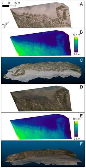
Figure 4.
(A) Orthomosaic constructed with data from survey 4 conducted on 20 January 2017; (B) Digital Elevation Model (DEM) of survey 4; (C) Screenshot of dense point cloud made with data from survey 4; (D) Orthomosaic constructed with data from survey 6 conducted on 12 January 2017; (E) DEM of survey 6; (F) Screenshot of dense point cloud made with data from survey 6. Scale bar in (A) also applied to (B,D,E).
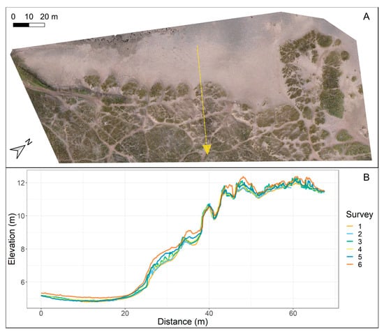
Figure 5.
(A) Orthomosaic constructed with data from survey 5 (conducted on 16 June 2017) overlaid with a transect; (B) Elevation profiles of the transect constructed with data from DEMs of all 6 KAP surveys.
3.1. Drone versus KAP Survey
Survey 6 with the KAP setup and the drone survey were undertaken on the same day and within one hour of each other. The drone flight covered part but not all of the area of interest (Figure 6A and Figure S2). The two surveys were compared to evaluate the relative uncertainties within both the drone and KAP methods, especially as the positioning of the sensor and resulting image overlap varied between the two (Figure 6B,C). In x, y and z dimensions, M3C2-PM precision estimations were smaller for the dense cloud constructed with data from the drone survey compared to the KAP survey (Table 2). Mean precision estimates were approximately 6 times greater for points in the KAP cloud in x and y dimensions (e.g., 31.3 mm and 29.5 mm respectively). For the z axis, mean precision estimations were almost 10 times greater in the KAP cloud at 87.9 mm (Table 2). DEMs created for the subset area used for this comparison show overall elevational range of 9.8 m, with sandy beach areas on the western edge and foredunes running approximately SW-NE (Figure 6D,E). The mean difference between the two DEMs was 30.7 mm, and the 5% and 95% quantiles were −41 mm and 177.3 mm respectively (Figure 6F). Beyond differences between DEMs, M3C2-PM was conducted using the dense clouds from each survey, to create a change point cloud (Figure 6G). Within this change cloud, 19% of points had significant differences, of these 89% were positive (showing greater elevation in the kite survey than the drone survey) and 11% negative (Figure 7). The distribution of significant change points was bi-modal, falling either side of 0 (no change; Figure 7), with a mean of 160 mm. The greatest differences between the point clouds derived from the KAP survey and drone survey were on stabilised and mostly vegetated parts of the dunes (Figure 6G), the positive differences greater (median: 128 mm; maximum: 313.6 mm) than negative differences (mean: −56 mm; maximum: −48 mm).
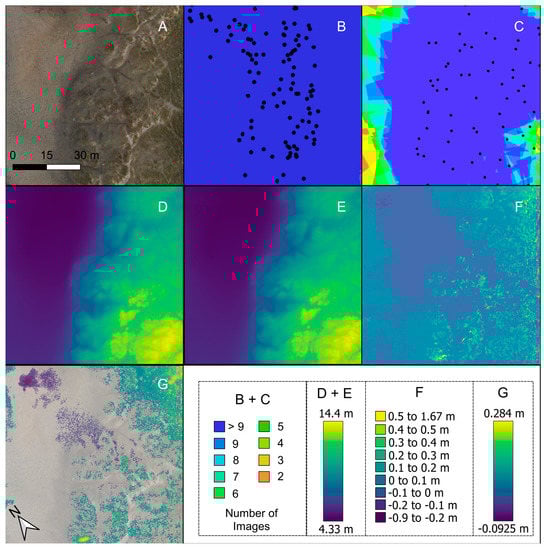
Figure 6.
Comparisons between KAP survey 6 and the drone survey (A) An orthomosaic created from images captured in KAP survey 6; (B) Image overlap for the KAP survey (taken from Photoscan report); (C) Image overlap for the drone survey (taken from Photoscan report). Black dots show estimated camera positions; (D) Digital elevation model (DEM) for the KAP survey; (E) DEM for the drone survey; (F) A DEM of difference between the KAP and drone DEMs; (G) Rasterised representation (spatial resolution of 0.1 m for display purposes) of significant results from M3C2-PM change analysis between point clouds created with data from KAP and drone surveys (overlaid on orthomosaic (at 50% transparency) from panel (A). Non-significant change points are absent from (G).
Table 2.
M3C2-PM derived precision estimations for the points contained in the KAP versus drone subset area of interest (Figure S2).
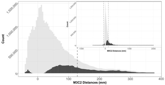
Figure 7.
Distribution of M3C2 distances between the kite survey and drone survey. Main figure shows data cropped to 5% and 95% quantiles with inset histogram showing all data. Points falling outside the common area between surveys have been removed, as they cannot be used in M3C2 analysis. Point cloud exported at native resolution of drone derived point cloud. Light grey shows all points in the change cloud and darker grey indicates significant changes in distance. Dashed lines indicate the positive (128 mm) and negative (−56 mm) median values of significant changes.
3.2. KAP Surveys
Considering all KAP surveys, the number of useable (e.g., non-blurry and without humans/animals) images collected in each survey varied from 374 (52% of the total collected during survey 6) to 774 (64% of the total collected during survey 2). Camera positions were calculated in Agisoft Photoscan, (rather than using the camera’s internal GPS unit) providing estimated x and y positions alongside the altitude at which each image was captured. The mean altitude was 36.9 m with 5% and 95% quartiles showing as 19 m and 56.8 m respectively (Figure S5). The accuracy of the point clouds when compared to check points for validation varied between surveys. Four ground control points were withheld for validation in each survey dataset, to assist in understanding the total error in products produced by the SfM-MVS workflow (compared to the D-GNSS measurements). Root mean square error (RMSE) calculated across x, y and z dimensions for all check points for each survey show that error was higher in surveys 4 and 5 (39.7 and 44.0 mm) than the other four surveys (ranged 15.9–18.9 mm; Table S2). The higher RMSE in survey 4’s check points was driven mainly by one point, especially in the z dimension (117.4 mm), whereas for survey 5, z dimension RMSE were higher for all points than seen in the other surveys (Table S2). Total RMSE calculated with error from all check points for all surveys was 19.7 mm in the horizontal (x/y), 39.4 mm in the vertical (z) and 27.9 across all (x/y/z) domains.
3.3. Intra-Annual Variation
Three pairs of surveys (1 & 2 (pair 1), 2 & 3 (pair 2) and 3 & 4 (pair 3)) were undertaken approximately 3 months apart (Table 1). In all 3 pairs of surveys, the majority of significant change across the dune system was positive (accretion), indicating elevational gain in the survey undertaken at the later date of the 2 in a pair. For all 3 surveys, more of the significant change was positive than negative (Table 3). Whilst most of the change in pairs 1 and 2 was between 0–500 mm, 40% points in pair 3 showed negative change (erosion) of between 0–500 mm (Table 3). Significant changes in elevation between surveys 1 & 2 were distributed across the whole area of interest whereas they were more concentrated in results from surveys 2 & 3 (Figure 8). There was far less significant change in pair 3 compared to pairs 1 and 2, with most of it negative and situated in areas of foredune. The mean positive change for each of the 3 months comparisons was pair 1: 121.8 mm, pair 2: 218.3 mm and pair 3: 197.7 mm.
Table 3.
Proportions of total number of significant points in M3C2-PM change rasters between pairs of surveys. Rasters were created from change clouds at a resolution of 0.75 m, with the mean of intersecting points in horizontal space assigned as the value in each cell.
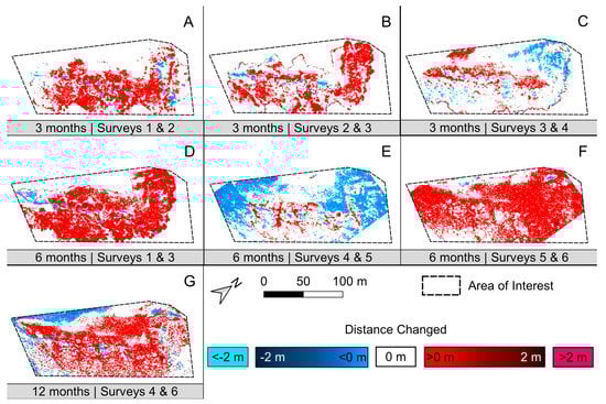
Figure 8.
Significant differences indicated by M3C2-PM comparisons between pairs of dense clouds. Changes were mostly between −2 and 2 m as indicated by the split colour ramps. Rasters were created from change clouds at a resolution of 0.75 m, with the mean of intersecting points in horizontal space assigned as the value in each cell and cropped to the area of interest (Figure 1). Panels (A–G) show rasterised M3C2-PM differences for pairs of surveys explored in intra- and inter-annual KAP comparisons.
Three pairs of surveys (1 & 3 (pair 1), 4 & 5 (pair 2) and 5 & 6 (pair 3)) were undertaken approximately 6 months apart (Table 1). Significant gain in sand dune elevation (accretion) was seen in the M3C2 results for pair 1, both in foredune areas and further inland (Figure 8). For pair 2, the north-eastern and south-western sides of the area of interest were concentrated areas of significant reduction in elevation, generally between 0–500 mm. For pair 3, elevational changes were almost exclusively positive and seen across the whole area of interest (Figure 8). Most of this change (97% of significantly changed points) was between 0–500 mm (Table 3). The mean significant positive change for pair 1 and pair 3 was 199.8 mm and 229.1 mm respectively. The mean negative change (erosion; as these were more numerous than positive changes) in survey pair 2 was −178.1 mm.
3.4. Inter-Annual Variation
Surveys 4 and 6 were conducted in January of 2017 and 2018 respectively (Table 1) providing an opportunity to explore change over a period of 12 months. The majority of significant change in this period was positive (accretion), with nearly 74% of points in the change cloud in the 0–500 mm category (Table 3). Some negative change (erosion) was also detected, with approximately 20% of points showing elevation reduction of between 0 to −500 mm (Table 3). The majority of negative changes were on the seaward side of the area of interest, whereas positive changes were seen along the dune fronts and further back towards the more stabilised part of the ecosystem (Figure 8).
3.5. Change within Specific Features
In order to further understand how specific components of the dune ecosystem changed in topography over time, beach, foredune and path areas were investigated on an inter-annual timescale. Of the three chosen features, points in beach areas experienced the lowest proportion of significant change compared to the total number of points sampled (42%). The majority of points in foredune and path environments changed significantly over 12 months, with 72% in foredunes and 83% on paths (Figure 9). Within beach features, significant change was exclusively positive with a mean of 130 mm change (Figure 9). For foredunes, the distribution was bimodal (median positive = 254 mm, median negative = −75 mm), although the majority of change was still positive (Figure 9). Change on footpaths was also bimodal (median positive = 388 mm, negative = −164 mm), but the distances (amount of change) were much greater than the other two features, with a range of −290 mm to 980 mm (Figure 9).
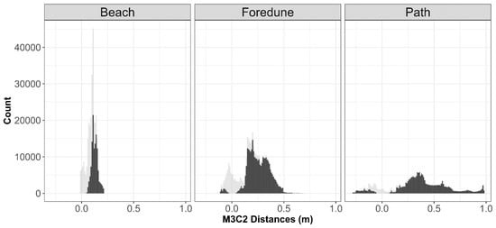
Figure 9.
Analysis of M3C2 change clouds for specific features within the study system. Change was calculated between surveys 4 and 6 (12 month timespan). Histograms show the distribution of all points (light grey) overlaid with the distribution of significant change points (dark grey) for each of the three features (beach, foredune, path) analysed.
4. Discussion
Here we have described the novel coupling of KAP for data capture with M3C2-PM analysis to track fine spatial scale changes in a coastal dune environment. We also provide a direct comparison of point clouds created with data from a lightweight multirotor drone and a KAP setup. The experimental design applied here, employing M3C2 analysis has allowed for consideration of repeatability (KAP versus drone) on the same date, assuming a consistent measurand, and between-date reproducibility to be quantified and taken into account (intra- and inter-annual KAP surveys). We argue that this is particularly important when the survey methodology (KAP) is likely to be affected by differing conditions at the time of each survey (wind, kite height, angular acquisition properties) such that consistent survey grid designs (as could be delivered from a drone or other aerial platform) are not guaranteed. In the subsequent sections, we discuss the major findings of the experiment and place these in the broader context of coastal monitoring using KAP based proximal sensing.
4.1. Drone versus KAP Survey
First, the assessment of the point cloud precision estimates (Table 2) showed that individual drone and KAP surveys captured on the same date exhibited precision estimates below 90 mm in all dimensions across both techniques. Precision estimates for the drone-derived point cloud were exceptionally small, and whilst the KAP precision estimates were greater they were still small at ~30 mm horizontally and 90 mm vertically. Even though the precision estimates of the KAP are higher (Table 2) the overall uncertainties are still small in magnitude. Comparing these results to one of the most commonly used methods for coastal topographic monitoring (airborne LiDAR), we have demonstrated that the KAP method can deliver orthomosaics with ~6 mm spatial resolution and point clouds with greater accuracy (x/y: 19.7 mm, z: 39.4 mm (see Table S2)). This exceeds the current typical capability of a the UK Environment Agency LiDAR system which generally have a spatial resolution of approximately 250 mm, and poorer z (150 mm) and x/y (400 mm) RMSE derived accuracy estimations [53]. Importantly, the level of precision shown in the KAP data is still suitable from a dune management point of view, where topographic change upwards of the decimetre scale is likely to be of interest.
Second, our results show that despite data collection at very similar periods of time (less than 60 min between flights), M3C2-PM analysis still highlighted topographical differences between the point clouds. On the more stabilised vegetated parts of the dune system, topography in the drone survey was more elevated than data from the KAP survey. The predominant type of vegetation in this zone of the dune system is Marram grass, which is easily moved in windy conditions, most likely explaining differences seen in these areas. Negative differences between the drone and KAP point clouds (5% quantile −42 mm) were of a smaller magnitude than positive differences (95% quantile 380 mm) (Figure 7). Most of these points were located within the foredune and beach zones, which although had high estimated image overlap (>9; Figure 6B,C), the KAP survey contained more images in this area compared to the drone. The differences seen between the drone and the KAP survey also highlight the presence of methodological uncertainty in proximal sensing techniques. The position of the sensor when it captured images of the study system most likely drove this difference between the resultant point clouds. The drone survey was flown with a ‘cross-hatch’ pattern meaning that parallel lines 90 degrees from each other were used as a flight path, with the aim to increase the number of viewing angles of features on the ground, and the drone camera geometry was fixed at nadir. The kite survey was walked across the study system with a less control resulting in less evenly spaced camera positions than the drone survey (after image quality checks and subsequent removal) (Figure 6B,C). Furthermore, the design of the picavet mount meant that the sensor could swing, naturally providing varying viewing angles during data capture with the KAP system, whereas the drone provided a more level platform. We also acknowledge that lighting conditions would have varied between these two surveys, driven by both sun angle and the level of cloud at the time of survey (see also Section 4.4). Despite these identified differences in methodology, there was a far greater proportion of cloud points that were not significantly different between the KAP and drone surveys (81%), compared to those that were (19%).
4.2. KAP Surveys
The time-series analysis of intra- and inter-annual KAP survey data evidenced that the majority of change in the dune system, both positive and negative topographic change, was small in absolute magnitude (less than 500 mm accretion or erosion; Table 3). Furthermore, despite the measurement uncertainties, the M3C2 analysis showed that the KAP survey method was capable of measuring these changes since they were highlighted as being significant (i.e., exceeding the point-based uncertainty measures). Finally, the mixture of 3-, 6- and 12-month comparisons demonstrate how KAP can be used to monitor change in coastal systems over different timescales and at different times of year where pressures on the system may differ. For example, within the 3 month datasets, the period between pairs 1 and 2 was characterised by enhanced tourist activity, when visitor numbers, and thus, trampling pressures were higher. In contrast the inter-annual survey encompasses change from a multitude of sources throughout the season including weather events and human activity.
The variety in camera positions (in x, y, z) between the 6 KAP surveys resulted in irregular spatial extent in the point cloud, orthomosaics (Figure S3) and DEMs (Figure S4) produced from the SfM-MVS workflow. Given that the majority of the area of interest was covered in each survey, the irregularity in coverage found with the KAP survey method was not an issue for M3C2-PM analysis. Furthermore the M3C2-PM technique does not require the exact matching of data points in space to conduct change analysis between point clouds, and also provides more spatially heterogenous error assessment compared to difference of DEM techniques [43]. The technique is therefore well suited for survey-to-survey variable measurement uncertainty, such as comparing methodologies or multi-temporal change analysis as is presented in this study.
The presence of Marram grass and other dune vegetation likely drove the changes in elevation detected in stabilised parts of the dune system between pairs of surveys. For example, the difference between surveys 1 & 2 exhibited positive elevational changes in areas behind the foredunes, where Marram grass is present (Figure 8 and Figure S3). These surveys were conducted in March and June 2016, a period of Spring to Summer transition where vegetation in the dune environment ‘greens up’. In this experiment we used only a RGB sensor so vegetation metrics (e.g., normalised difference vegetation index (NDVI)) could not be determined. However, we suggest that including infra-red based vegetation index data such as NDVI could be used to further enhance the M3C2-PM analysis by separating vegetation from bare sand areas to improve identification of the more dynamic parts of the dune environment, as has been shown by Reference [36].
4.3. KAP as a Tool for Coastal Monitoring
Conducting proximal sensing topographic surveys in coastal dune environments is not a trivial task. First, with reference to the positioning of GCPs, there are very few static features that can be utilised as known points in space between surveys. In this case we managed to measure the positioning of two fixed features (concrete base and an entrance stone). Leaving GCPs for more than half a day was not a feasible option due to the risk of human interference. For one survey presented in this study, one GCP was removed by a member of the public only hours after being placed. However, the financial gains (compared to other coastal monitoring techniques) and fine temporal resolution offered with proximal sensing make this a valuable tool for monitoring the coastal environment [54].
The windy conditions found at the coast (Figure 2) make KAP a useful alternative proximal sensing technique when compared to drones (which are more difficult to operate in windy conditions). Their ease-of-use, low-cost [55] and less strict regulation surrounding their use make the technique a democratic and appropriate technology [29]. When collecting data for an SfM-MVS workflow, we have shown that KAP can be an advantageous platform for optical sensors due to the variation in camera position created by movement of the kite, shown by the larger precision estimations calculated in the Monte Carlo processing stage (Table 2). This in turn offers oblique viewing angles of features on the ground which helps reproduce steep sided features (such as those found in dunes) which may be absent in nadir images, especially when the features are orthogonal to the sensors’ orientation. Furthermore oblique imagery reduces the doming effect sometimes visible in SfM-MVS data products [56].
4.4. Other Sources of Uncertainty
As we stated at the beginning of the discussion, the method followed allowed us to consider various sources of measurement uncertainty, both within (i.e., precision/repeatability; Table 2) and between surveys (i.e., reproducibility (e.g., Figure 8 and Table 3), and with reference to independent checkpoints surveyed with a D-GNSS (Table S2). The M3C2-PM technique takes into account sources of calibration (e.g., internal camera sensor calibration), equipment (specific camera performance) and method (e.g., accuracy of GCP locations) uncertainty relating to the collection and processing of SfM-MVS data and propagates these through the analysis. However, other sources should also be considered including operator and environment related uncertainties. Here the same operator (author JPD) conducted all surveys and so we cannot quantify this within our experiment, but we suggest that it would be important to consider if multiple kite operators were used. This may be particularly pertinent in the event that KAP surveys were used as a crowdsourcing data collection effort. Uncertainties related to the environmental conditions under which the measurements were collected can manifest as differences in (i) sky illumination (potentially explaining differences between the KAP and drone survey in this study), (ii) reflectance of wet/dry surfaces relating to weather conditions prior to and during the survey, (iii) wind conditions affecting the position of vegetation, and (iv) the presence of aerosols (airborne sand or salt particles). We argue that these scene- and site-dependent environmentally-driven uncertainties will have been captured to some extent within the large dataset analysed and so are likely accounted for within the M3C2-PM results. Disaggregating their individual impacts is impossible without undertaking a series of separate experiments where those parameters are varied individually, and the impacts quantified. This lies outside of the scope of our work but could form the basis of a series of interesting follow-up studies.
5. Conclusions
It is in the interest of coastal communities and populations in general to maintain high quality sand dune systems, especially in vulnerable coastal environments. Dunes and their associated vegetation communities can help form part of a realistic and sustainable coastal protection system [57]. The impacts of disturbances in dune systems such as trampling until now have focused largely on the changes in plant communities [9], but less on changes to dune structure. Given that trampling can lead to the destabilization of dune systems [1], there is a need to monitor change in topography over time. Sand dunes are highly dynamic and change rapidly over time, and thus a flexible method that allows for data capture are user-dictated times makes KAP a well-suited method for dune monitoring efforts. Furthermore, the technique presented in this study can be readily deployed by others to monitor changes in dune topography in relation to anthropogenic disturbance events alongside the monitoring of natural change over time. From a management point of view, one could perform KAP surveys before and after interventions such as fencing or signposting to understand their effectiveness in preserving environmental integrity. This approach lends itself to the implementation of proactive rather than reactive interventions, allowing managers to monitor coastal environments at temporal scales tailored to their specific needs. Our approach also shows that specific areas (i.e., foredune) can be specifically analysed to aid in the understanding of change in specific parts of dune systems. This work develops that of [19,58,59,60] but takes a more robust quantitative approach to multi-temporal monitoring by accounting for many forms of uncertainty with the M3C2-PM methodology.
Beyond monitoring natural dynamic coastal environments, the technique could also be used to monitor movement and/or damage to structures such as jetties, rock defences, sea walls and other property. For example, the effects of storm damage to sea walls could be detected immediately post storm in a cost-effective manner that doesn’t require airborne LiDAR or TLS capabilities, in turn reducing the cost of surveying. KAP is a low-cost, self-service, highly-portable technique that has lower barriers to entry than other proximal sensing techniques (e.g., drone technology). When applied at relevant spatial and temporal scales KAP is a powerful data capture method well suited for monitoring coastal environments.
Supplementary Materials
The following are available online at http://www.mdpi.com/2072-4292/10/9/1494/s1, dune_ms_supp_figures.docx (containing all supplementary figures), dune_ms_supp_tables.docx (containing all supplementary tables), dune_ms_agisoft_photoscan_and_m3c2_workflow.docx (containing detailed methods descriptions) and Photoscan reports for all KAP and the drone survey.
Author Contributions
Conceptualization, J.P.D., J.D.S., K.A.; Methodology, J.P.D., M.J.W., L.D., K.A.; Software, J.P.D., M.J.W., L.D.; Validation, J.P.D.; Formal Analysis, J.P.D.; Investigation, J.P.D., K.A.; Resources, J.P.D., M.J.W., K.A.; Data Curation, J.P.D.; Writing—Original Draft Preparation, J.P.D.; Writing—Review & Editing, J.P.D., J.D.S., M.J.W., L.D., K.A.; Visualization, J.P.D.; Supervision, J.P.D., J.D.S., M.J.W., K.A.; Project Administration, J.P.D.; Funding Acquisition, J.P.D., J.D.S., K.A.
Funding
This research was funded by [Natural Environment Research Council] grant number [570009815].
Data Access Statement
The research data supporting this publication are openly available from the University of Exeter’s institutional repository at: https://doi.org/10.24378/exe.723.
Acknowledgments
We would like to thank Colin Anderson, Jonathan Crocker, Ned Crowley, Sarah Crowley, Joel Forsmoo, Cecily Goodwin, Darren Jones, Nicole Parr, and Polly Shutler for their assistance with data collection. Also, thank you to Cornwall Council for allowing us to conduct research on the St. Gothian Sands Local Nature Reserve. We are grateful to Mike James (Lancaster University) for his guidance with data processing and analysis and Peter Land (Plymouth Marine Laboratory) for constructive comments on the manuscript. We also thank three anonymous reviewers and the editor for their constructive comments which have improved the manuscript.
Conflicts of Interest
The authors declare no conflict of interest.
References
- Barbier, E.B.; Hacker, S.D.; Kennedy, C.; Koch, E.W.; Stier, A.C.; Silliman, B.R. The value of estuarine and coastal ecosystem services. Ecol. Monogr. 2011, 81, 169–193. [Google Scholar] [CrossRef]
- Hardisty, J. Beach and nearshore sediment transport. In Sediment Transport and Depositional Processes; Pye, K., Ed.; Blackwell: London, UK, 1994; pp. 216–255. [Google Scholar]
- Hesp, P. Foredunes and blowouts: Initiation, geomorphology and dynamics. Geomorphology 2002, 48, 245–268. [Google Scholar] [CrossRef]
- Sigren, J.M.; Figlus, J.; Highfield, W.; Feagin, R.A.; Armitage, A.R. The Effects of Coastal Dune Volume and Vegetation on Storm-Induced Property Damage: Analysis from Hurricane Ike. J. Coast. Res. 2018, 34, 164–173. [Google Scholar] [CrossRef]
- Acosta, A.; Carranza, M.L.; Izzi, C.F. Are there habitats that contribute best to plant species diversity in coastal dunes? Biodivers. Conserv. 2009, 18, 1087–1098. [Google Scholar] [CrossRef]
- Everard, M.; Jones, L.; Watts, B. Have we neglected the societal importance of sand dunes? An ecosystem services perspective. Aquat. Conserv. Mar. Freshw. Ecosyst. 2010, 20, 476–487. [Google Scholar] [CrossRef]
- Defeo, O.; McLachlan, A.; Schoeman, D.S.; Schlacher, T.A.; Dugan, J.; Jones, A.; Lastra, M.; Scapini, F. Threats to sandy beach ecosystems: A review. Estuar. Coast. Shelf Sci. 2009, 81, 1–12. [Google Scholar] [CrossRef]
- Brown, A.C.; McLachlan, A. Sandy shore ecosystems and the threats facing them: Some predictions for the year 2025. Environ. Conserv. 2002, 29, 62–77. [Google Scholar] [CrossRef]
- Santoro, R.; Jucker, T.; Prisco, I.; Carboni, M.; Battisti, C.; Acosta, A.T.R. Effects of Trampling Limitation on Coastal Dune Plant Communities. Environ. Manag. 2012, 49, 534–542. [Google Scholar] [CrossRef] [PubMed]
- Lemauviel, S.; Rozé, F. Response of Three Plant Communities to Trampling in a Sand Dune System in Brittany (France). Environ. Manag. 2003, 31, 227–235. [Google Scholar] [CrossRef] [PubMed]
- Davidson-Arnott, R.; Hesp, P.; Ollerhead, J.; Walker, I.; Bauer, B.; Delgado-Fernandez, I.; Smyth, T. Sediment budget controls on foredune height: Comparing simulation model results with field data. Earth Surf. Process. Landf. 2018, 43, 1798–1810. [Google Scholar] [CrossRef]
- Roelvink, D.; Reniers, A.; van Dongeren, A.; van Thiel de Vries, J.; McCall, R.; Lescinski, J. Modelling storm impacts on beaches, dunes and barrier islands. Coast. Eng. 2009, 56, 1133–1152. [Google Scholar] [CrossRef]
- Feagin, R.A.; Williams, A.M.; Popescu, S.; Stukey, J.; Washington-Allen, R.A. The Use of Terrestrial Laser Scanning (TLS) in Dune Ecosystems: The Lessons Learned. J. Coast. Res. 2014, 30, 111–119. [Google Scholar] [CrossRef]
- Smith, A.; Gares, P.A.; Wasklewicz, T.; Hesp, P.A.; Walker, I.J. Three years of morphologic changes at a bowl blowout, Cape Cod, USA. Geomorphology 2017, 295, 452–466. [Google Scholar] [CrossRef]
- Schubert, J.E.; Gallien, T.W.; Majd, M.S.; Sanders, B.F. Terrestrial Laser Scanning of Anthropogenic Beach Berm Erosion and Overtopping. J. Coast. Res. 2015, 31, 47–60. [Google Scholar] [CrossRef]
- Buckley, S.J.; Howell, J.A.; Enge, H.D.; Kurz, T.H. Terrestrial laser scanning in geology: Data acquisition, processing and accuracy considerations. J. Geol. Soc. 2008, 165, 625–638. [Google Scholar] [CrossRef]
- Westoby, M.J.; Brasington, J.; Glasser, N.F.; Hambrey, M.J.; Reynolds, J.M. ‘Structure-from-Motion’ photogrammetry: A low-cost, effective tool for geoscience applications. Geomorphology 2012, 179, 300–314. [Google Scholar] [CrossRef]
- Zhang, C.; Kovacs, J.M. The application of small unmanned aerial systems for precision agriculture: A review. Precis. Agric. 2012, 13, 693–712. [Google Scholar] [CrossRef]
- Westoby, M.J.; Lim, M.; Hogg, M.; Pound, M.J.; Dunlop, L.; Woodward, J. Cost-effective erosion monitoring of coastal cliffs. Coast. Eng. 2018, 138, 152–164. [Google Scholar] [CrossRef]
- Hugenholtz, C.H.; Levin, N.; Barchyn, T.E.; Baddock, M.C. Remote sensing and spatial analysis of aeolian sand dunes: A review and outlook. Earth Sci. Rev. 2012, 111, 319–334. [Google Scholar] [CrossRef]
- Li, J.; Roy, D.P. A Global Analysis of Sentinel-2A, Sentinel-2B and Landsat-8 Data Revisit Intervals and Implications for Terrestrial Monitoring. Remote Sens. 2017, 9, 902. [Google Scholar] [CrossRef]
- Rader, A.M.; Pickart, A.J.; Walker, I.J.; Hesp, P.A.; Bauer, B.O. Foredune morphodynamics and sediment budgets at seasonal to decadal scales: Humboldt Bay National Wildlife Refuge, California, USA. Geomorphology 2018, 318, 69–87. [Google Scholar] [CrossRef]
- Stockdon, H.F.; Sallenger, A.H., Jr.; List, J.H.; Holman, R.A. Estimation of Shoreline Position and Change Using Airborne Topographic Lidar Data. J. Coast. Res. 2002, 18, 502–513. [Google Scholar] [CrossRef]
- Burningham, H.; French, J. Understanding coastal change using shoreline trend analysis supported by cluster-based segmentation. Geomorphology 2017, 282, 131–149. [Google Scholar] [CrossRef]
- Bazzichetto, M.; Malavasi, M.; Acosta, A.T.R.; Carranza, M.L. How does dune morphology shape coastal EC habitats occurrence? A remote sensing approach using airborne LiDAR on the Mediterranean coast. Ecol. Indic. 2016, 71, 618–626. [Google Scholar] [CrossRef]
- Chust, G.; Galparsoro, I.; Borja, Á.; Franco, J.; Uriarte, A. Coastal and estuarine habitat mapping, using LIDAR height and intensity and multi-spectral imagery. Estuar. Coast. Shelf Sci. 2008, 78, 633–643. [Google Scholar] [CrossRef]
- Mumby, P.J.; Green, E.P.; Edwards, A.J.; Clark, C.D. The cost-effectiveness of remote sensing for tropical coastal resources assessment and management. J. Environ. Manag. 1999, 55, 157–166. [Google Scholar] [CrossRef]
- Anderson, K.; Gaston, K.J. Lightweight unmanned aerial vehicles will revolutionize spatial ecology. Front. Ecol. Environ. 2013, 11, 138–146. [Google Scholar] [CrossRef]
- Duffy, J.P.; Anderson, K. A 21st-century renaissance of kites as platforms for proximal sensing. Prog. Phys. Geogr. 2016, 40, 352–361. [Google Scholar] [CrossRef]
- Cunliffe, A.M.; Brazier, R.E.; Anderson, K. Ultra-fine grain landscape-scale quantification of dryland vegetation structure with drone-acquired structure-from-motion photogrammetry. Remote Sens. Environ. 2016, 183, 129–143. [Google Scholar] [CrossRef]
- Ota, T.; Ogawa, M.; Shimizu, K.; Kajisa, T.; Mizoue, N.; Yoshida, S.; Takao, G.; Hirata, Y.; Furuya, N.; Sano, T.; et al. Aboveground Biomass Estimation Using Structure from Motion Approach with Aerial Photographs in a Seasonal Tropical Forest. Forests 2015, 6, 3882–3898. [Google Scholar] [CrossRef]
- Mancini, F.; Dubbini, M.; Gattelli, M.; Stecchi, F.; Fabbri, S.; Gabbianelli, G. Using Unmanned Aerial Vehicles (UAV) for High-Resolution Reconstruction of Topography: The Structure from Motion Approach on Coastal Environments. Remote Sens. 2013, 5, 6880–6898. [Google Scholar] [CrossRef]
- Duffy, J.P.; Pratt, L.; Anderson, K.; Land, P.E.; Shutler, J.D. Spatial assessment of intertidal seagrass meadows using optical imaging systems and a lightweight drone. Estuar. Coast. Shelf Sci. 2018, 200, 169–180. [Google Scholar] [CrossRef]
- Sturdivant, E.J.; Lentz, E.E.; Thieler, E.R.; Farris, A.S.; Weber, K.M.; Remsen, D.P.; Miner, S.; Henderson, R.E. UAS-SfM for Coastal Research: Geomorphic Feature Extraction and Land Cover Classification from High-Resolution Elevation and Optical Imagery. Remote Sens. 2017, 9, 1020. [Google Scholar] [CrossRef]
- Otero, V.; Van De Kerchove, R.; Satyanarayana, B.; Martínez-Espinosa, C.; Fisol, M.A.; Ibrahim, M.R.B.; Ibrahim, S.; Mohd-Lokman, H.; Lucas, R.; Dahdouh-Guebas, F. Managing mangrove forests from the sky: Forest inventory using field data and Unmanned Aerial Vehicle (UAV) imagery in the Matang Mangrove Forest Reserve, peninsular Malaysia. For. Ecol. Manag. 2018, 411, 35–45. [Google Scholar] [CrossRef]
- Nolet, C.; Van Puijenbroek, M.; Suomalainen, J.; Limpens, J.; Riksen, M. UAV-imaging to model growth response of marram grass to sand burial: Implications for coastal dune development. Aeolian Res. 2018, 31, 50–61. [Google Scholar] [CrossRef]
- Madurapperuma, B.; Close, P.; Fleming, S.; Collin, M.; Thuresson, K.; Lamping, J.; Dellysse, J.; Cortenbach, J. Habitat Mapping of Ma-le’l Dunes Coupling with UAV and NAIP imagery. Proceedings 2018, 2, 368. [Google Scholar] [CrossRef]
- Duffy, J.P.; Cunliffe, A.M.; Debell, L.; Sandbrook, C.; Wich, S.A.; Shutler, J.D.; Myers-smith, I.H.; Varela, M.R.; Anderson, K. Location, location, location: Considerations when using lightweight drones in challenging environments. Remote Sens. Ecol. Conserv. 2018, 4, 7–19. [Google Scholar] [CrossRef]
- Fraser, W.R.; Carlson, J.C.; Duley, P.A.; Holm, E.J.; Patterson, D.L. Using Kite-Based Aerial Photography for Conducting Adélie Penguin Censuses in Antarctica. Waterbirds 1999, 22, 435–440. [Google Scholar] [CrossRef]
- Feurer, D.; Planchon, O.; El Maaoui, M.A.; Slimane, A.; Boussema, M.R.; Pierrot-Deseilligny, M.; Raclot, D. Using kites for 3-D mapping of gullies at decimetre-resolution over several square kilometres: A case study on the Kamech catchment, Tunisia. Nat. Hazards Earth Syst. Sci. 2018, 18, 1567–1582. [Google Scholar] [CrossRef]
- Bryson, M.; Johnson-Roberson, M.; Murphy, R.J.; Bongiorno, D. Kite Aerial Photography for Low-Cost, Ultra-high Spatial Resolution Multi-Spectral Mapping of Intertidal Landscapes. PLoS ONE 2013, 8, e73550. [Google Scholar] [CrossRef] [PubMed]
- Lague, D.; Brodu, N.; Leroux, J. Accurate 3D comparison of complex topography with terrestrial laser scanner: Application to the Rangitikei canyon (N-Z). ISPRS J. Photogramm. Remote Sens. 2013, 82, 10–26. [Google Scholar] [CrossRef]
- James, M.R.; Robson, S.; Smith, M.W. 3-D uncertainty-based topographic change detection with structure-from-motion photogrammetry: Precision maps for ground control and directly georeferenced surveys. Earth Surf. Process. Landf. 2017, 42, 1769–1788. [Google Scholar] [CrossRef]
- Natural England St Gothian Sands LNR. Available online: https://designatedsites.naturalengland.org.uk/SiteLNRDetail.aspx?SiteCode=L1122976&SiteName=G&countyCode=6&responsiblePerson=&SeaArea=&IFCAArea= (accessed on 1 March 2018).
- CHDK Development Team Canon Hack Development Kit. Available online: http://chdk.wikia.com/wiki/CHDK (accessed on 17 September 2018).
- James, M.R.; Robson, S.; D’Oleire-Oltmanns, S.; Niethammer, U. Optimising UAV topographic surveys processed with structure-from-motion: Ground control quality, quantity and bundle adjustment. Geomorphology 2017, 280, 51–66. [Google Scholar] [CrossRef]
- Harvey, P. Exiftool: Read, Write and Edit Meta Information! Available online: http://owl.phy.queensu.ca/~phil/exiftool/ (accessed on 17 September 2018).
- Baddeley, A.; Rubak, E.; Turner, R. Spatial Point Patterns: Methodology and Applications with R; Chapman and Hall/CRC Press: London, UK, 2015. [Google Scholar]
- R Core Team. R: A Language and Environment for Statistical Computing; R Core Team: Vienna, Austria, 2017. [Google Scholar]
- Agisoft LLC Photoscan Professional (1.3.1). 2017. Available online: http://www.agisoft.com/ (accessed on 17 September 2018).
- Pebezma, E.; Bivand, R.; Rowlingson, B.; Gomez-Rubio, V.; Hijmans, R.; Sumner, M.; MacQueen, D.; Lemon, J.; O’Brien, J.; O’Rourke, J. Sp: Classes and Methods for Spatial Data, R Package Version 1.2-5; 2017. Available online: http://www.et.bs.ehu.es/cran/web/packages/sp/index.html (accessed on 17 September 2018).
- CloudCompare (Version 2.10) [GPL Software]. 2017. Available online: https://www.danielgm.net/cc/ (accessed on 17 September 2018).
- Environment Agency. Environment Agency LIDAR Data: Technical Note; Environment Agency: Bristol, UK, 2016.
- Gonçalves, J.A.; Henriques, R. UAV photogrammetry for topographic monitoring of coastal areas. ISPRS J. Photogramm. Remote Sens. 2015, 104, 101–111. [Google Scholar] [CrossRef]
- Conlin, M.; Cohn, N.; Ruggiero, P. A Quantitative Comparison of Low-Cost Structure from Motion (SfM) Data Collection Platforms on Beaches and Dunes. J. Coast. Res. 2018. [Google Scholar] [CrossRef]
- James, M.R.; Robson, S. Mitigating systematic error in topographic models derived from UAV and ground-based image networks. Earth Surf. Process. Landf. 2014, 39, 1413–1420. [Google Scholar] [CrossRef]
- Feagin, R.A.; Figlus, J.; Zinnert, J.C.; Sigren, J.; Martínez, M.L.; Silva, R.; Smith, W.K.; Cox, D.; Young, D.R.; Carter, G. Going with the flow or against the grain? The promise of vegetation for protecting beaches, dunes, and barrier islands from erosion. Front. Ecol. Environ. 2015, 13, 203–210. [Google Scholar] [CrossRef]
- Autret, R.; Dodet, G.; Suanez, S.; Roudaut, G.; Fichaut, B. Long-term variability of supratidal coastal boulder activation in Brittany (France). Geomorphology 2018, 304, 184–200. [Google Scholar] [CrossRef]
- Bryson, M.; Duce, S.; Harris, D.; Webster, J.M.; Thompson, A.; Vila-Concejo, A.; Williams, S.B. Geomorphic changes of a coral shingle cay measured using Kite Aerial Photography. Geomorphology 2016, 270. [Google Scholar] [CrossRef]
- Seymour, A.C.; Ridge, J.T.; Rodriguez, A.B.; Newton, E.; Dale, J.; Johnston, D.W. Deploying Fixed Wing Unoccupied Aerial Systems (UAS) for Coastal Morphology Assessment and Management. J. Coast. Res. 2018, 34, 704–717. [Google Scholar] [CrossRef]
© 2018 by the authors. Licensee MDPI, Basel, Switzerland. This article is an open access article distributed under the terms and conditions of the Creative Commons Attribution (CC BY) license (http://creativecommons.org/licenses/by/4.0/).