1. Introduction
Snow has important relevance for society spanning from environmental and economical to recreational and aesthetic values. Environmentally snow influences the climate and ecology of an area through its effect on solar energy absorption and by constraining land cover characteristics [
1,
2]. Snowmelt results in significant decrease of surface albedo and releases the water stored in seasonal snowpack, providing water for humans and the environment [
3,
4]. Water managers in hydropower and water supply sectors consider snow storage in mountain areas as a natural reservoir [
5]. During the past decades, hydrological models have been used to assess the amount and spatiotemporal distribution of this important resource [
6,
7]. However, the modeling process in general and model calibration in particular is prone to various sources of uncertainty [
8]. Further, the objective functions commonly used for parameter inference using inverse modeling are based on aggregate measures of model performance and usually yield to poorly constrained model parameters [
9]. A combined approach of model calibration followed by data assimilation is one of the strategies commonly followed to deal with model uncertainty [
10,
11]. Data assimilation (DA) is the means to obtain an estimate of the true state through use of independent observations and the prior knowledge (model state) with appropriate uncertainty modeling [
9,
12].
Ensemble-based filtering and smoothing techniques are commonly used in solving DA problems [
9]. The filtering techniques involve updating of state variables and/or parameter values at each observation time with subsequent production of error statistics that can be cycled to future analysis times; while in smoothing all observations are assimilated in a single step [
4,
13]. Some of the filtering- (sequential) based DA schemes commonly used in hydrological data assimilation include the Ensemble Kalman Filter [
14] and the Particle filter [
15], while some examples from the smoother-based DA schemes include the ensemble batch smoother [
16] as well as the particle batch smoother (Pbs) [
17]. The smoother-based DA schemes have the advantage of low computational cost coupled with the flexibility in running independent of the forward model [
4,
18,
19].
In recent years, remote sensing data in general and optical fractional snow cover area (fSCA) in particular has been increasingly used in hydrologic modeling for constraining model parameters through inverse modeling and various DA schemes [
20]. This can be attributed to the readily available observations of this data for large areas and at a relatively high temporal resolution [
21,
22]. In DA, fSCA has been used from a simple rule-based (direct-insertion) approach [
23] to advanced filtering and smoothing techniques [
24,
25]. The collection of fSCA measurements and their temporal evolution during the ablation period reflect the peak snow water equivalent (SWE) better than a single fSCA measurement does. Hence, the batch assimilation techniques are preferable over filtering techniques when the assimilated observation is fSCA in a snow depletion curve model [
17]. The Pbs and particle filter DA schemes have been gaining interest as fSCA assimilation schemes in snow models due to their distribution free likelihood and their capability to estimate the SWE state vector directly at a relatively low computational cost [
17,
26]. However, these schemes assume crisp and equal informational value for all observations of the assimilated data. Further, in these schemes, most of the weights are assigned to one or very few ensemble members and this may lead to degeneration of the statistical information in the ensembles [
27,
28]. An alternative approach that ensures fair distribution of weights among ensemble members is the limits of acceptability (LoA) [
29]. This approach provides flexibility in choosing different shapes for representing the error within specified error bounds. It further allows the incorporation of different hydrological signatures in the evaluation criteria. As such, it is more process-based as compared to the simple residual-based objective functions since it transforms the observed and simulated data into hydrologically relevant signatures [
30].
In this study, the informational value of fSCA measurements is considered to be fuzzy, carrying a considerable amount of uncertainty. In previous studies different approaches have been used to increase the amount of information that can be extracted from time series data during parameter inference using inverse modeling [
30]. Some of these measures include: breaking up the time series data into different periods, for example, the different components of a hydrograph [
31] as well as transforming the time series data to emphasise on some aspects of the system response [
32]. In several snow related DA studies all measurements are assumed to carry the same amount of information in constraining the model states and parameters. However, the amount of information that can be extracted from remote sensing data varies depending on several factors including the presence of certain physical limitations such as clouds and lack of sufficient light [
33]. For example, high latitudes are characterized by polar darkness and frequent cloud cover and errors emanating from such sources can reduce the informational value of MODIS fSCA product for snow assimilation [
34,
35].
The informational value of MODIS fSCA was divided into three timing windows; and an automatic change point (CP) detection scheme was employed to identify the spatially and temporally variable location of the CP in the time-axis. CP detection deals with the estimation of the point at which the statistical properties of a sequence of observations changes [
36]. In hydrology, CP detection methods have been applied in various studies including the assessment of non-stationarity in time series data [
37,
38] as well as in the assessment of flow-solute relationship in water quality studies [
39]. Nevertheless, their application has been limited when it comes to the analysis of remote sensing snow cover data. Although, snowmelt at high latitudes is a rapid process, the start date of an ablation period may vary by several weeks from year to year in response to such factors as the amount of accumulated SWE before the onset of snowmelt and the availability of melt energy [
40]. Spatially, the onset of snow melt varies from one grid-cell to another depending on variability in physiographic characteristics of the area in addition to the above mentioned climatic factors. During the accumulation period, spatial variability of snow results from snow-canopy interaction in forested areas, snow redistribution by wind, and orographic effects [
41]. During the ablation period, snow melts from preferential locations, yielding heterogeneous patterns [
42].
The main goal of this study is to get an improved estimate of SWE during the maximum accumulation period using fuzzy logic-based ensemble fSCA assimilation schemes and by incorporating uncertainties in selected model forcing and parameters. The first objective is to assess whether the assumption of variable informational value of fSCA observations depending on their location in different timing windows can reduce the uncertainty in SWE reanalysis. We introduce a novel approach that accommodates this concept by incorporating a fuzzy coefficient in the ensemble-based SWE reanalysis schemes. The second objective is to evaluate the viability of statistical change point detection methods to locate the critical points that constitute the timing windows. The third objective is to compare effect of the assumed variability in informational value of fSCA observations on relative performance of the Pbs and the LoA-based DA schemes. As of our best knowledge, the LoA approach was not used before for DA purposes; and this study will assess the feasibility of this approach as an ensemble smoother DA scheme.
This paper is organized as follows.
Section 2 presents the snow model followed by description of the study area as well as the static and time-series data used in this study. This section also presents setup of the different DA schemes and methodologies followed to detect the critical dates in the ablation period. Results from the DA schemes in comparison to the observed values as well as sensitivity of the evaluation metrics to location of the change points in the ablation period are presented in
Section 3. Finally, certain points from the methodology and results sections are discussed in
Section 4 in light of previous studies; and relevant conclusions are drawn in
Section 5.
2. Methods and Materials
2.1. The Hydrological Model
The forward model used in this study, PT_GS_K, is a conceptual hydrological model (method stack) within the Statkraft Hydrological Forecasting Toolbox (Shyft,
https://github.com/statkraft/shyft). This model and the modeling framework were described in previous studies [
43,
44] and this section presents main features of the model with focus on its snow method. PT_GS_K encompasses the Priestley–Taylor (PT) method [
45] for estimating potential evaporation; a quasi-physical-based snow method (GS) for snow melt, sub-grid snow distribution and mass balance calculations; and a simple storage-discharge function (K) [
46,
47] for catchment response calculation.
PT_GS_K operates on a single snow layer and it can be forced by hourly or daily meteorological inputs of precipitation, temperature, radiation, relative humidity, and wind speed. The Model uses a Bayesian Kriging approach to distribute the point temperature data over the domain, while for the other forcing variables it uses an inverse distance weighting approach. The model generates streamflow, fSCA, and SWE as output variables.
The potential evaporation calculation in the PT method requires net radiation, the slope of saturated vapor pressure, the Priestley–Taylor parameter, the psychometric constant, and the latent heat of vaporization [
48]. Actual evapotranspiration is assumed to take place only from snow free areas and it is estimated as a function of potential evapotranspiration and a scaling factor.
The energy balance calculation in GS method follows a similar approach as used by DeWalle and Rango [
49] (Equation (1)). The precipitation falling in each grid-cell is classified as solid or liquid precipitation depending on a threshold temperature (
tx) and on the local temperature values. The available net snow melt energy (
) is the sum effect of different energy sources and sinks in the system. These include: incoming short wave radiation (
), incoming (
) and outgoing (
) long wave radiation, the subsurface energy flux (
) as well as the turbulent sensible (
) and latent (
) energy fluxes emanating from rainfall, solar radiation, wind turbulence and other sources.
Among other factors, the energy contribution from short wave radiation depends on snow albedo. For a given time step (
t), the snow albedo of each grid cell depends on the minimum (
) and maximum (
) albedo values as well as on air temperature (
) (Equation (2)). In this method the decay rates of albedo due to snow aging as a function of temperature, i.e., the fast (
) and slow (
) albedo decay rates corresponding to temperature conditions above and below 0 °C respectively, are parameterized [
50].
The incoming and outgoing longwave radiations are estimated based on the Stephan–Boltzmann law. Turbulent heat contribution is the sum of latent and sensible heat. Wind turbulence is linearly related to wind speed using a wind constant and wind scale from the intercept and slope of the linear function, respectively [
50]. The subsurface energy flux is a function of snow surface layer and the snow surface temperature.
The sub-grid snow distribution in each grid cell is described by a three parameter Gamma probability distribution snow depletion curve (SDC) [
51,
52]. This SDC is based on the assumption that certain proportion of a grid cell area (
) remains snow-free throughout the winter season such as in steep slopes and ridges due to wind erosion or avalanches [
53]. As such, the two parameter Gamma distribution function, characterized by the average amount of snow
(mm) and the sub-grid snow coefficient of variation (
) at the onset of the melt season (Equation (3)), is applied only to the remaining portion of a grid cell area to estimate the fraction of the initially snow covered area where snow has disappeared (
). Following this formulation, the bare ground fraction at each time step (
is estimated using Equation (4).
where,
denotes the Gamma probability density function and
is the incomplete Gamma function with shape
and scale
. The variables
and
respectively refer to point snow storage and the accumulated melt depth (mm) at time t since the onset of the melt season.
Although, the catchment response function (K) was used for estimating the regional model parameter values through calibration against observed streamflow data, this method was not directly employed in this study.
2.2. Study Area and Data
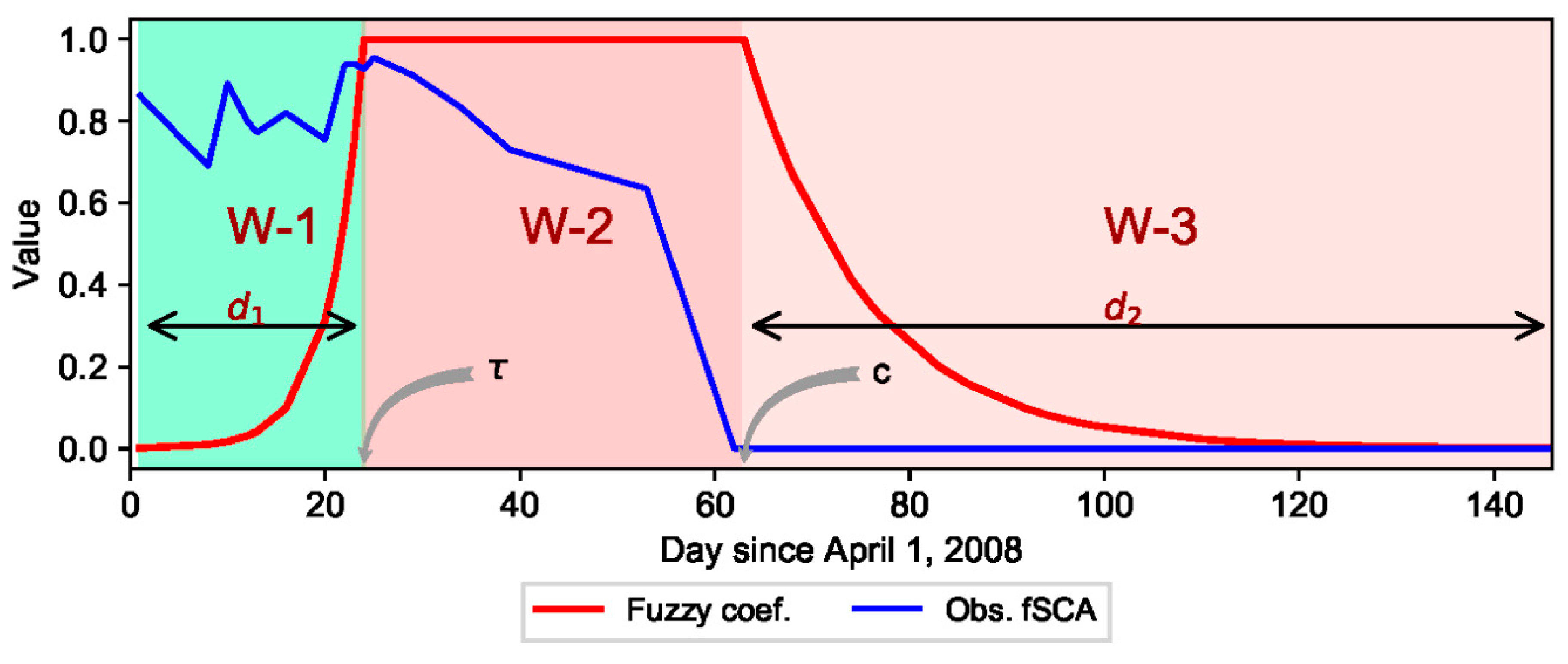
The study sites are located in Nea-catchment, Sør-Trøndelag County, Norway (
Figure 1). The Nea-catchment covers a total area of 703 km
2 and its geographical location ranges from 11.67390° to 12.46273° E and from 62.77916° to 63.20405° N. Altitude of the study sites ranges from around 700 masl at site-1 to above 1200 masl at site-7. The fact that the model was previously setup for the study area plus the availability of long term SWE data, i.e., for nine years and in nine different sites, make the Nea-catchment an appealing study area to apply the DA schemes. The observed SWE data cover the hydrological years 2008–2016; and the datasets in these years were used in validating the DA schemes. The highest and lowest average catchment peak SWE values estimated from the nine sites during these hydrological years were 717 and 331 mm respectively in years 2012 and 2014. Mean annual precipitation for the nine hydrological years was 1279 mm. The highest and lowest average daily temperature values for this period were 20 and −23 °C, respectively.
The SWE reanalysis was conducted on 33 grid cells located at nine sites (
Table 1). The location of these grid-cells was constrained by the availability of snow course measurements in the catchment. Daily time series data of most meteorological forcing variables, i.e., temperature, precipitation, radiation, and wind speed were obtained from Statkraft [
54] as point measurement, while daily gridded relative humidity data were retrieved from ERA-interim [
55]. Different physiographic and observational datasets were also used to generate the simulation results and in subsequent reanalysis using the DA schemes as well as during evaluation of the results. The model was setup over each grid cells of 1 km
2; requiring average elevation, grid cell total area, as well as the areal fraction of forest cover. Data for these physiographic variables were retrieved from two sources: the land cover data from Copernicus land monitoring service [
56] and the 10m digital elevation model (10m DEM) from the Norwegian mapping authority (Kartverket.no). The land cover data show that, the catchment is mainly dominated by moors, heathland and some sparse vegetation; and only limited part of the catchment is forest covered (3%). The grid cells considered in the DA study are located on the open areas of the catchment. The median SWE data of each grid cell were derived from radar measurements provided by Statkraft [
54]. The data were collected once a year in the month of April, where accumulated snow storage approximately attains its peak magnitude. The radar measurements roughly follow the same course each year in the nine representative sites of the catchment. Daily fraction of snow cover area (fSCA) was retrieved from NASA MODIS snow cover products [
57]. Frequent cloud cover is one of the major challenges when using MODIS and other optical remote sensing data in Norway. A composite dataset was thus formed using data retrieved from the Aqua and Terra satellites, MYD10A1 and MOD10A1 products respectively in order to minimize the effect of obstructions and misclassification errors emanating from clouds and other sources. The days with available snow cover data were used without filtering based on further criteria such as the remaining clouds. A direct assessment of the bias associated with this product was not done in this study as independent snow cover observations were not available for the study domain. The estimated annual average bias of these MODIS fSCA products for Northern Hemisphere is approximately 8 % in the absence of cloud [
58] and in forest dominated areas it may reach up to 15% [
59]. This MODIS product was reported to have a relatively lower accuracy as compared to other more recent products, e.g., the MODSCAG algorithm [
1] mainly due to its limited use of the available information in a given scene [
60].
2.3. The Data Assimilation Strategy
This section presents the perturbed forcing and model parameters followed by description of the two main DA schemes employed in this study, i.e., Pbs and LoA as well as other two similar versions of these schemes that take into account for variability in informational value of fSCA. The ensemble-based DA schemes involve two steps, namely prediction and updating. The prediction step provides the prior estimates of SWE using the dynamic (meteorological) and static (physiographic) forcings. In the updating step, the DA schemes are applied to constrain the prior SWE estimates using the fSCA observations and thereby yielding a posterior SWE estimates. Each grid cell is updated independently.
2.3.1. Perturbed Forcing and Model Parameters
In this study, one meteorological forcing and two model parameters are randomly perturbed to produce an ensemble of 100 model realizations. Precipitation was perturbed since meteorological forcing, in general and precipitation in particular, are the major sources of uncertainty in simulating snow storage and depletion processes [
61,
62]. Considering uncertainty in precipitation provides the means to control the amount of accumulated SWE in the absence of a viable spatial snow redistribution mechanism [
17]. The perturbed model parameters are sub-grid snow coefficient of variation (CV
s) and initial bare ground fraction (
). Snow coefficient of variation affects the SDC through its impact on the rate of snow depletion. In snow models with the sub-grid snow distribution component parameterized using statistical probability distribution function, the rate of snow depletion is inversely related to CV
s [
41]. Thus, when the sub-grid snow cover is more variable, the ground gets exposed earlier than when it is uniformly distributed [
20]. The initial bare ground fraction plays an important role in the SDC especially during the onset of snow melt when the fraction of initial snow covered area where snow has disappeared (
) is at its lowest [
52].
Both log-normal and logit-normal probability distributions are used to perturb the model forcing and parameters. A log-normal distribution was assumed for precipitation, while for CV
s and
a logit-normal distribution was assumed. A similar approach to previous SWE reanalysis studies [
17,
28] was followed in perturbing precipitation and the model parameters. Instead of directly perturbing the precipitation input at each time step (
), a perturbation parameter (
) was randomly generated from a log-normal distribution and the generated,
values are used as multiplicative biases for their respective ensemble member,
j (Equation (5)). Since the correction for wind induced precipitation under-catch was previously done, it was assumed that the average ensemble,
, value is unbiased with a value of unity. The snow coefficient of variation (CV
s) estimated during calibration of the model against observed streamflow was adopted as the prior mean value. The mean value of
was set to 0.04 based on previous studies in Norway [
52]; and its variability was kept to a narrow range, since this parameter can easily compensate for differences between the observed and simulated fSCA values [
52].
A standard deviation (
) of 15% was used to represent the measurement error in fSCA. This value is set based on previous studies focused on MODIS measurement errors [
59].
Table 2 presents the perturbation parameters and their assumed prior values.
2.3.2. fSCA Assimilation using Particle Batch Smoother
Previous studies indicate that the batch smoother is better suited than the filtering approach when dealing with SWE reanalysis through assimilation of fSCA observations [
17,
63]. A particle batch smoother (Pbs) uses an ensemble of independent randomly drawn Monte Carlo samples (particles) and estimates the posterior weight of each particle. The procedure involves generating ensemble of model realizations by running the model over the full seasonal cycle followed by the assimilation of all fSCA measurements at once. The Bayes theorem forms the basis for estimating the updated relative importance (weight,
wj) of each ensemble member (Equation (6)).
where
refers to the likelihood of the observations (y) given the state value of the jth ensemble member (
); and
denotes prior values.
In Pbs, all ensemble members are implicitly assigned equal prior weights of 1/Ne [
17]. When using the Gausian likelihood, this yields [
17,
28]:
where
and
respectively refer to
vector of perturbed fSCA observations and predicted fSCA for the
jth particle in the
matrix (
).
denotes
diagonal observation error covariance matrix.
Pbs assumes that both the prior and posterior states of the particles remain the same [
17]. It updates the particle weights in such a way that particles with their predictions closer to the observations get higher weight than those with farther from the observations. The median and prediction quantiles are estimated from the cumulative distribution of the sorted SWE values and their associated weights.
2.3.3. fSCA Assimilation Using the LoA
We use two hydrologic signatures to constrain the perturbation parameters by the LoA scheme through weighting the relative importance of the particles with a fuzzy rule. In a fuzzy rule, the information contained in a fuzzy set is described by its membership function [
64]. The first signature is based on the ability of each ensemble member to reproduce the observations within pre-defined error bounds of fSCA observations. The same value of measurement error as used in Pbs was also adopted here, i.e., 15% (
Table 2). The deviation between the observed and simulated values was converted into a normalized criterion using a fuzzy rule-based scoring function. A triangular membership function was assumed with its support representing the uncertainty in MODIS fSCA observations and the pointed core representing a perfect match between the observed and predicted fSCA (Equation (8)). The weight of each ensemble member with respect to this signature (
) is calculated as the membership grade of the prediction error, summed over all observations (Equation (9)).
where
is the membership grade of each prediction error
corresponding to the observed fSCA value
;
is the point in the support with perfect match between the observed and predicted fSCA values. The variables
and
respectively refer to the lower and upper bounds of the fSCA observation error.
The second hydrologic signature is based on the degree of persistency of an ensemble member in reproducing the observations. This is estimated by the percentage of observations (
) where the predicted values fall within the MODIS fSCA error bounds. Ensemble members whose prediction failed to reproduce at least 50% of the observations within the error bounds are considered as non-persistent and assigned a membership grade of zero. The degree of membership linearly increases for those that satisfy the condition from 50% to 95% of the observations; and attains its maximum value after 95%. Thus, ensemble members that are able to reproduce 95% to 100% of the observations within the error bounds are considered as the most persistent and accordingly assigned a membership grade of 1.0. The weight of each ensemble member with respect to its persistence in reproducing the observations (
) is equal to the degree of membership (
Equation 10). The combined weight (
) resulting from the two membership functions is determined by calculating the product of
and
followed by normalizing the result in such a way that all particle weights would sum up to 1.
where
is the membership grade of each ensemble member with respect to its persistency (
p) in reproducing the observations;
represents the minimum bound of the support (
p = 50%) and
refers to the point in the support where the membership grade starts to attain its maximum value (
p = 95%).
2.3.4. DA Schemes with an Account for Fuzzy Informational Value of fSCA
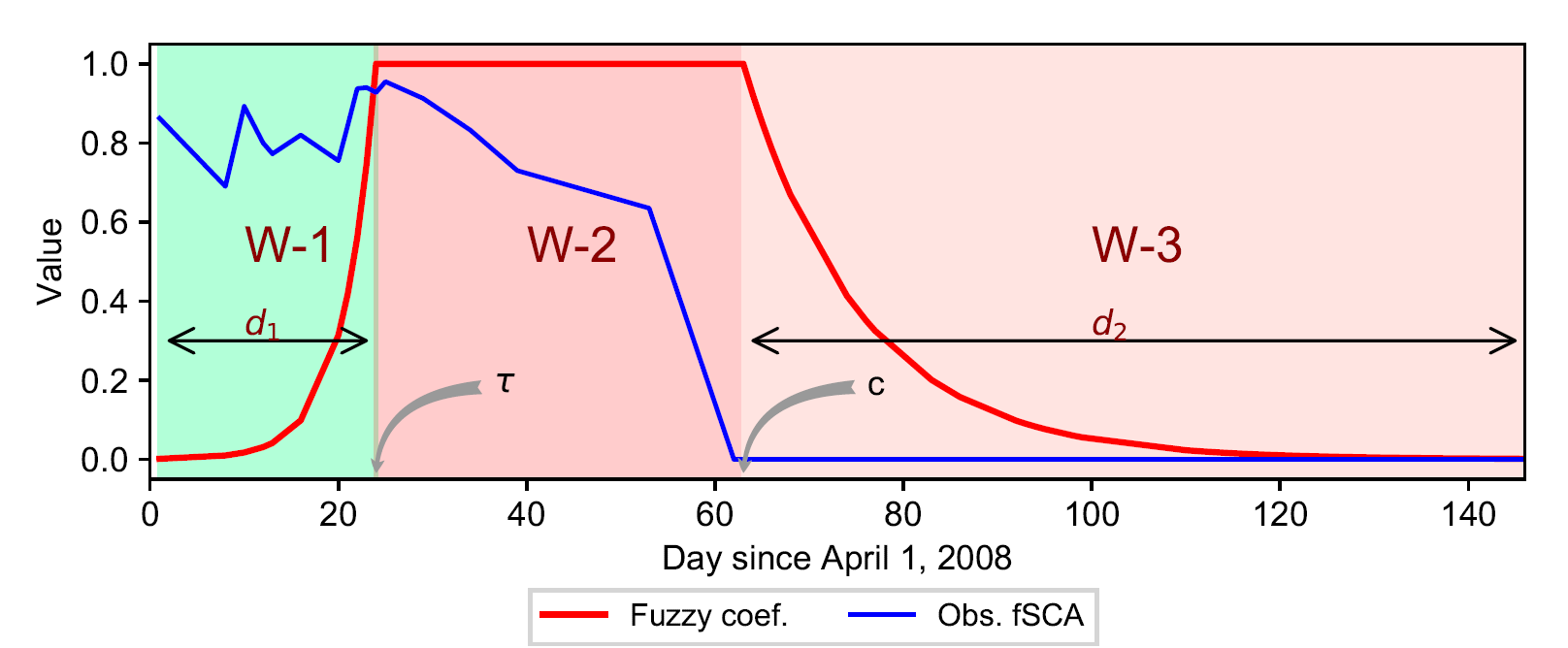
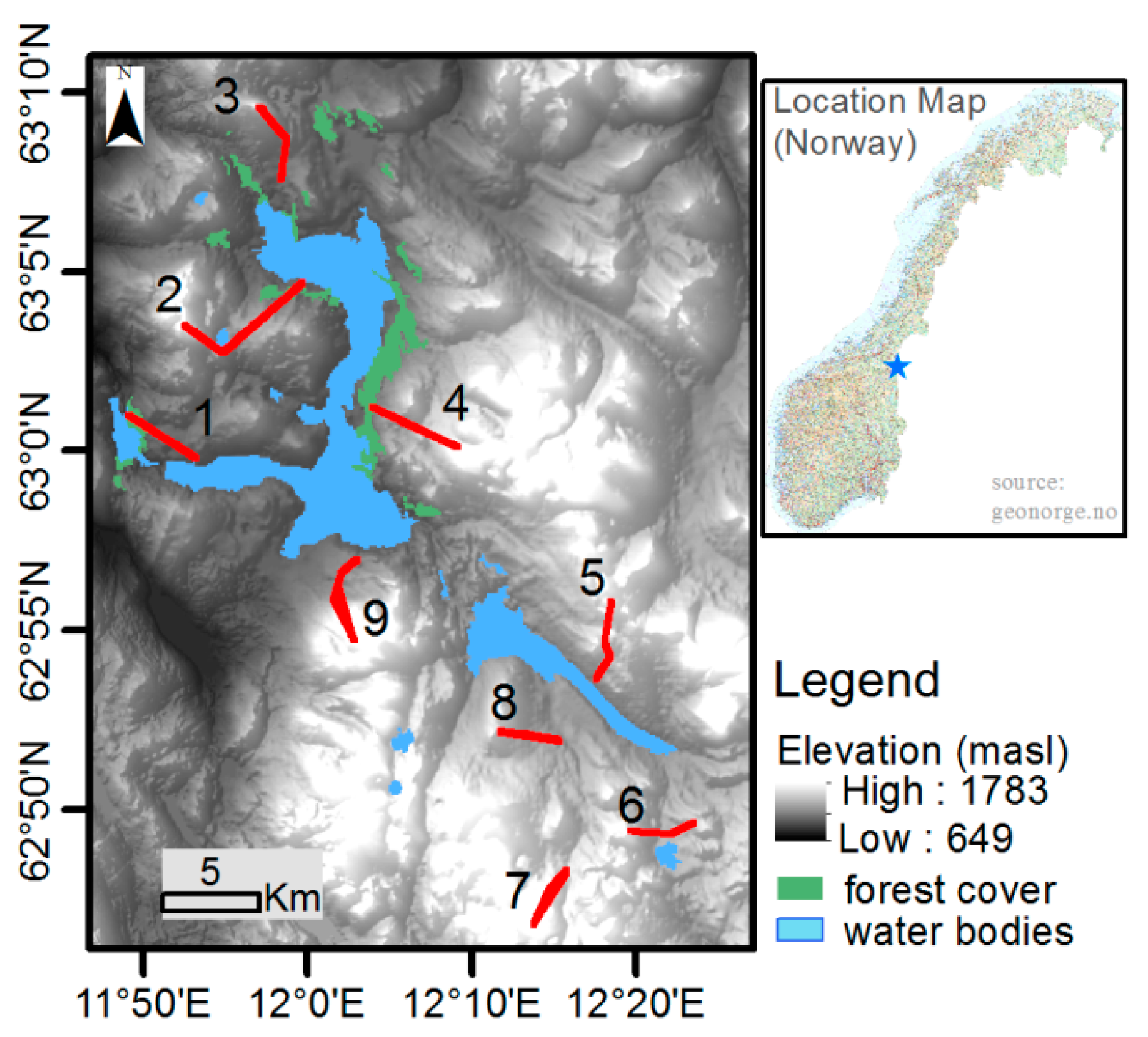
Here, the ablation period is divided into three timing windows with respect to the assumed relative informational value of fSCA observations (
Figure 2). This assumption is based on the concept that information is gained from an observation only if there is uncertainty about it; and an event that occurs with a high probability conveys less information and vice versa [
65]. The plot shows temporal distribution of fSCA for a sample grid-cell in the study area. The first timing window (W-1) is characterized by some snow melt with a subsequent decrease in SWE while the fSCA remains close to its maximum value. The fSCA observations from this window are characterized by low signal-to-noise ratio. In the second window (W-2), fSCA starts to drop at a faster rate and this window is characterized by high signal-to-noise ratio with a strong decreasing trend with time. The third window (W-3) corresponds to the complete melt-out period; and with the exception of few fSCA observations from sporadic snow events, fSCA is expected to remain null throughout this period. The fSCA observations in W-1 and W-3 are thus relatively certain, conveying less information as compared to observations in W-2.
The informational value of MODIS fSCA observation is considered to be fuzzy and varying with location of each observation in the time axis and with respect to the aforementioned conceptualization of the informational value of fSCA in the three timing windows. A fuzzy coefficient (α) was introduced in the original formulations of Pbs and the LoA schemes in order to account for the variability in informational value of fSCA on the DA results. This coefficient was described by a fuzzy degree of membership function whose value is greater than zero based on the assumption that all observations contribute certain information in constraining the perturbation parameters. An exponential trapezoidal membership function was adopted to describe α (Equation (11)). The informational value of the MODIS fSCA observations is assumed to exponentially increase in W-1 until it reaches end of this timing window at
. After start of the complete melt-out period (
), the informational value is assumed to exponentially decay with time in W-3. The fSCA observation is assumed to be most informative in the period between these two timing windows, i.e., in W-2. Hence, all observations in this period are assigned a maximum α value of unity.
where
is the membership grade of each fSCA observation date index (
);
and
respectively refer to the change point and start of the melt-out period in the time-axis.
and
respectively denote the widths of W-1 and W-3 in the time-axis.
The α value of each fSCA observation is equal to the membership grade corresponding to that observation (
); and this fuzzy coefficient is incorporated in the likelihood measure of Pbs in a way that it rescales the level of uncertainty of the residuals corresponding to each observation (Equation (12)).
For the LoA-based DA scheme, the membership grades of the fSCA prediction errors (, Equation (8)) were rescaled through multiplication by their respective α value before taking sum of . The remaining steps are similar to the procedure followed in the LoA scheme described earlier, i.e. to get the product of and with subsequent rescaling of the result in such a way that the weights of all ensemble members would sum up to unity.
2.4. Detection of Critical Periods with Respect to the Informational Values of fSCA
The critical dates that form the timing windows and the fuzzy coefficient curve (
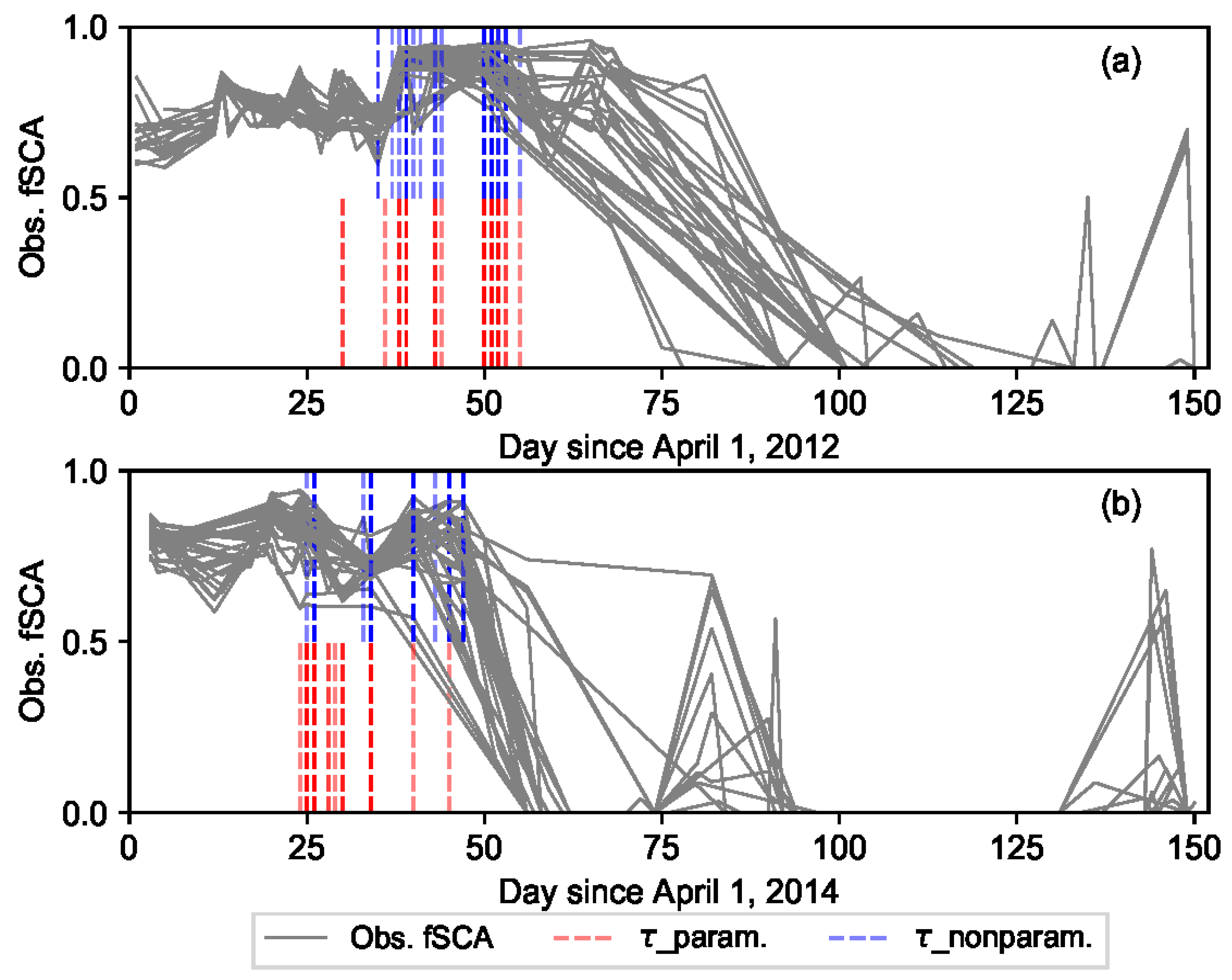
Figure 2) were identified using a change point detection algorithm. The two critical dates, i.e., the point in the time axis where the change in mean snow cover of a given grid-cell occurs and start of the melt-out period in that grid cell, vary from year to year; and spatially from one grid-cell to another in response to various climatic and physiographic characteristics of an area. The use of a flexible change point detection scheme is a viable option to address the impact of such spatially and temporally variable factors on critical dates and thereby on spatiotemporal variability of SWE. The timing for start of the melt-out period in each grid cell was identified as the first incident with null fSCA observation. Detection of the CP location was realized by performing an offline change point analysis using the likelihood-based parametric approach. For the sake of comparison, change points were also estimated using the non-parametric approach. In order to minimize effect of the noisy data, the change point detection methods were applied over the transformed fSCA data (cumulative sum of fSCA). This section describes the methodology followed in detecting the change points using these two approaches.
The CP detection schemes are based on the idea that given n ordered sequence of data,
, a change point is expected to occur within this set when there exists a time,
, such that the statistical properties (e.g., mean or variance) of
and
are different in some way. The parametric change point analysis scheme employed in this study was adopted from previous studies focused on implementation of the methodology based on the likelihood ratio [
36,
66,
67]. Change point detection was presented as a hypothesis test where the null hypothesis corresponds to no change in mean; while under the alternative hypothesis, a change point is expected to occur at time
. The parametric method based on the likelihood ratio requires the calculation of the maximum log-likelihood under both null and alternative hypotheses [
36]. Assuming the transformed fSCA data (
) as independent and normally distributed random variable, the likelihood ratio under the null (
) and alternative (
) hypotheses as well as the resulting log-likelihood ratio (
) can be described as follows.
where
,
and
respectively denote mean value of the transformed fSCA for the whole observation period, before the change point and after the change point.
refers to variance of the transformed fSCA data.
The generalized log-likelihood ratio
is estimated as:
The null hypothesis is rejected if , where is a predefined critical value; and the value of that maximizes is taken as the change point position. In this study the Bayesian Information Criterion (BIC) was employed to define this critical value, i.e., , where is the number of extra parameters used to define the change point (here = 1).
When performing the change point analysis using a nonparametric approach, the method of Taylor [
68] was followed. The procedure involves calculation of the cumulative sums (
) of the differences between the observations and their mean value (Equation (17)). The index in the time axis corresponding to the maximum cumulative sum (Equation (18)) is adopted as location of the change point
.
where
and
respectively refer to the transformed fSCA observations and their mean value. For the first observation
= 0 and the cumulative sum ends at
= 0.
The confidence level for the change point was determined by performing bootstrap analysis. First, the magnitude of the change is estimated as the difference between the maximum and minimum
(
). Then, N = 1000 bootstraps of
n observations are sampled through random reshuffling of the original data. For each bootstrap sample, the
values corresponding to each observation as well as the difference between the maximum and minimum
values (
) are calculated. Accordingly, the percentage confidence level (
) is estimated using Equation (19).
where,
2.5. Evaluation Metrics
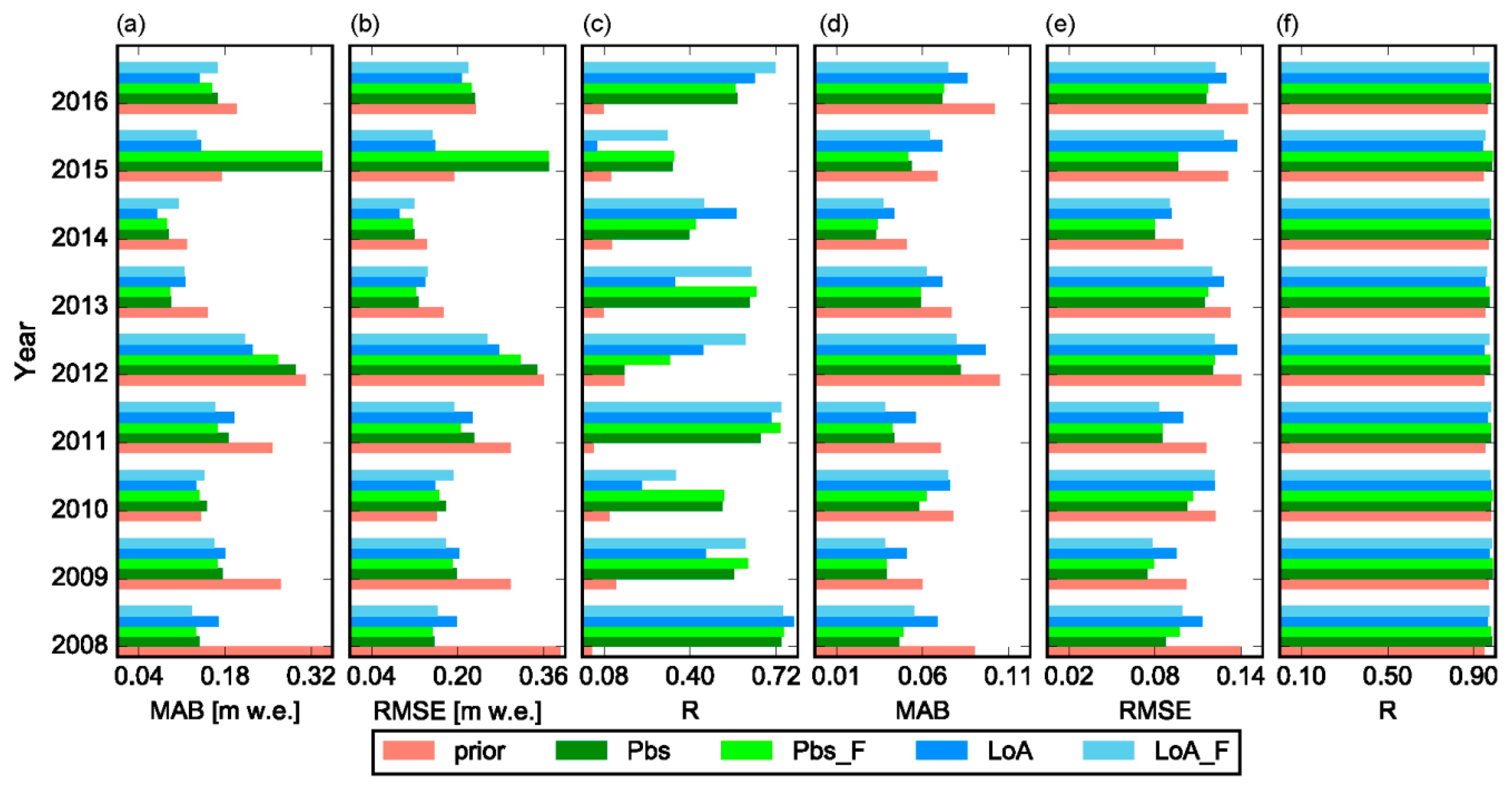
The performance of each DA scheme was evaluated through comparison of the median value of the ensemble predictions () against the observed () values. The following three evaluation metrics, i.e., mean absolute bias (), root mean of squared errors () as well as correlation coefficient () are employed during evaluation of estimated values against fSCA and SWE observations.
where
,
and N respectively refer to standard deviation, covariance, and the number of observations.
4. Discussion
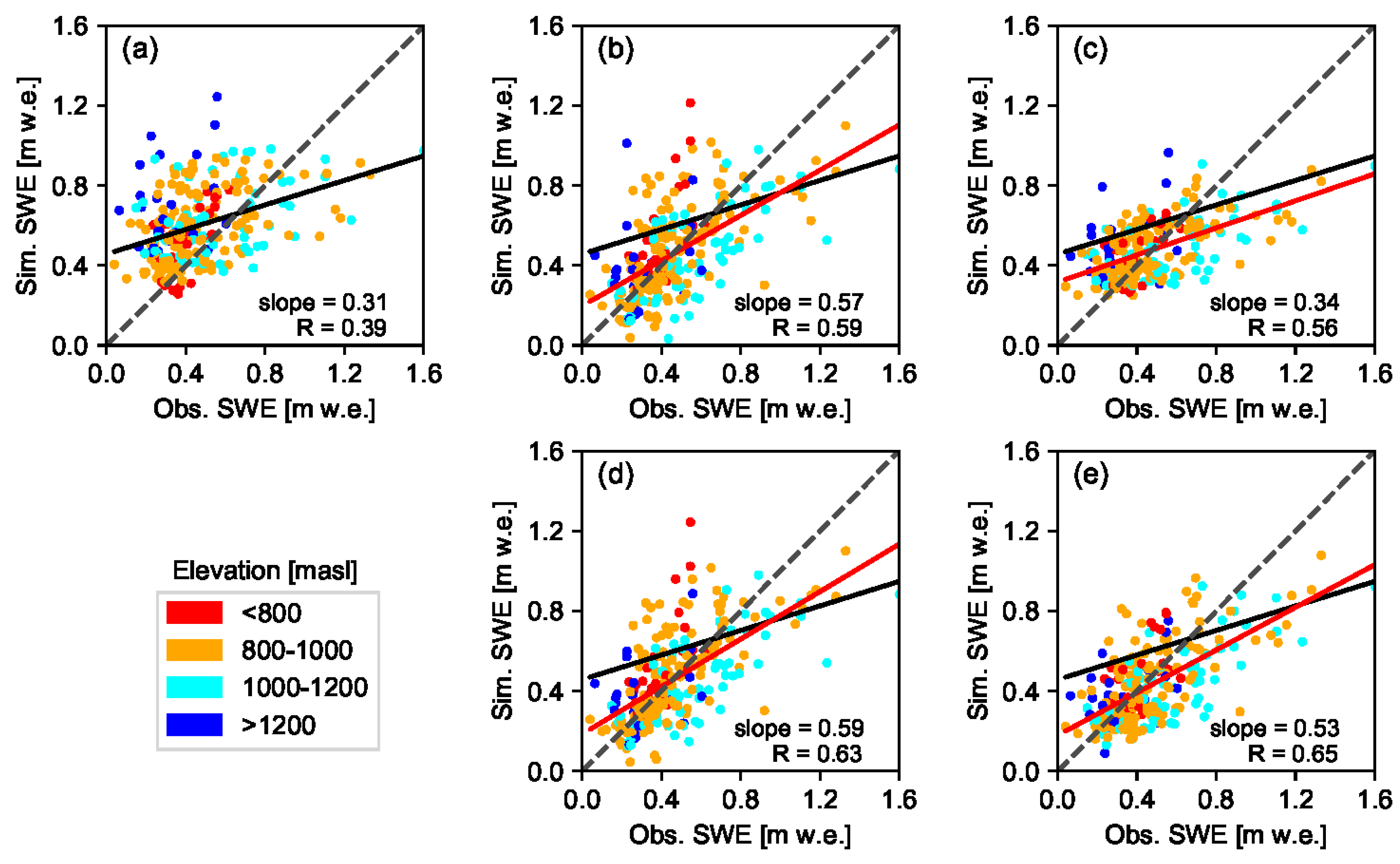
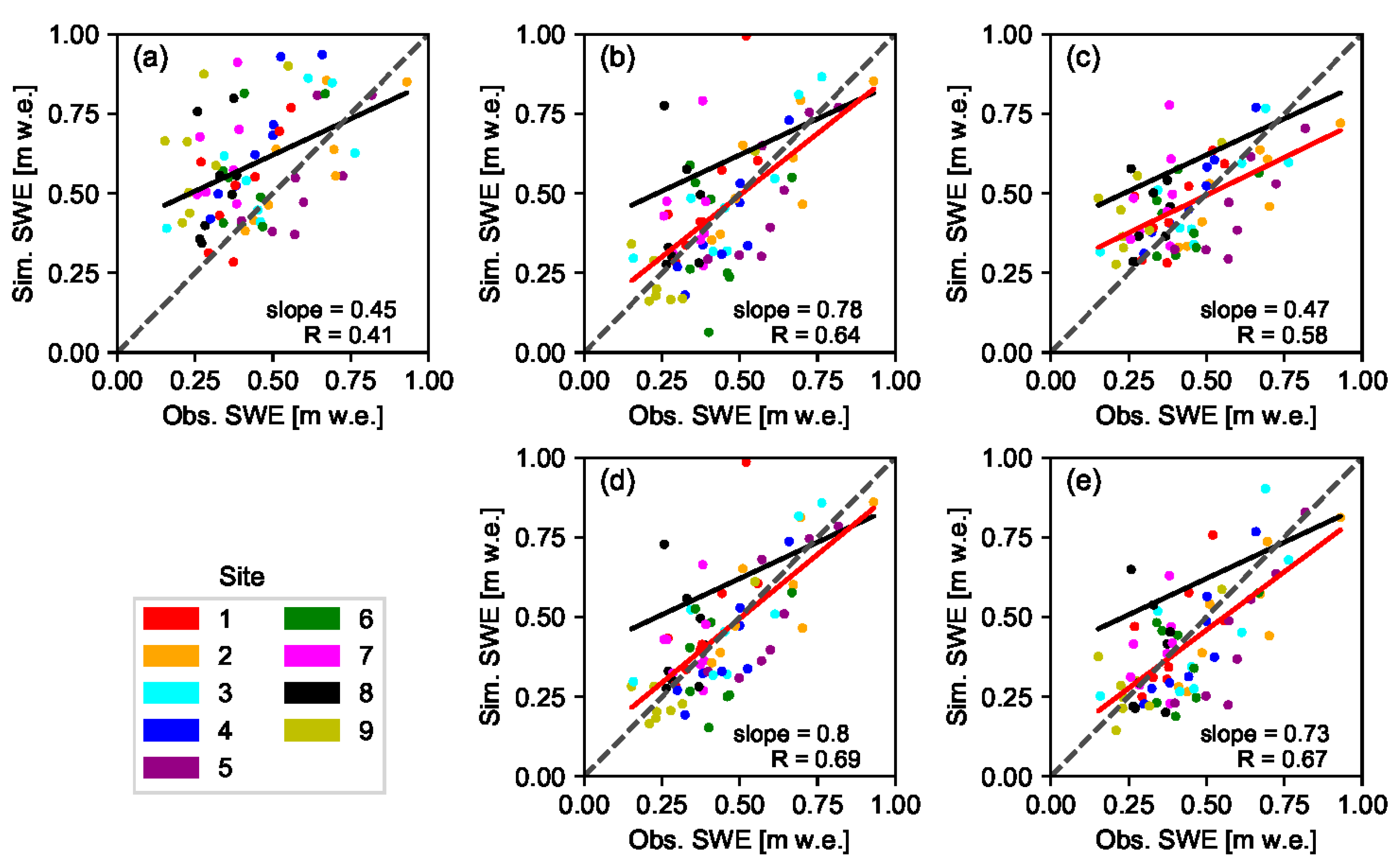
In this study four ensemble-based batch smoother schemes were used to retrospectively estimate SWE during the peak accumulation period through assimilation of fSCA into a snow hydrological model. Effect of the DA schemes was analyzed for nine years and with due consideration to different elevation zones as well as two spatial scales, i.e., at grid-cell and site levels. One of these schemes was based on a Bayesian approach (Pbs), while the other was based on the limits of acceptability concept (LoA). In both approaches, model predictions were scaled proportional to weight of each ensemble member. Due to nature of the likelihood function used, most of the weights in Pbs were carried by few ensemble members, while in the LoA framework, the weights were fairly shared by all ensemble members.
Although reanalysis using these DA schemes has yielded a significant improvement of the correlation coefficient in all analysis years, only a slight improvement was observed in most of these years when accuracy of the reanalyzed SWE was compared against the prior values based on the MAB and RMSE statistical criteria. The result was generally encouraging given the high level of uncertainty associated with remote sensing data in high latitude areas due to frequent clouds and polar darkness. Other similar studies focused on assimilation of MODIS fSCA into hydrological models have also reported only a modest improvement in SWE and streamflow estimates after assimilation; and it was mainly attributed to the very short transition period between the full snow cover and the complete melt-out dates [
24,
20]. On the other hand, studies based on the assimilation of multiple-source remote sensing data have reported significant improvement in these evaluation metrics [
28].
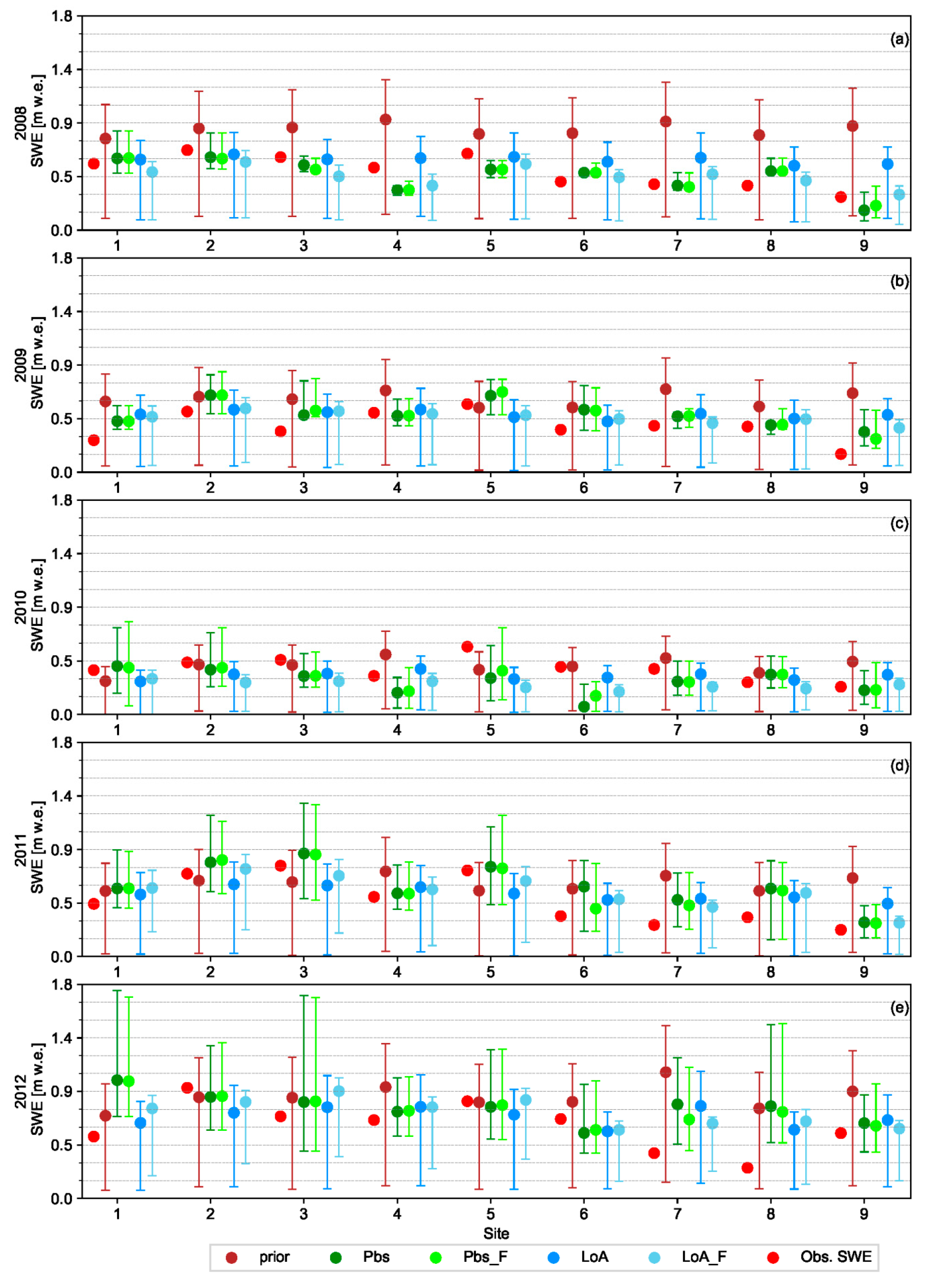
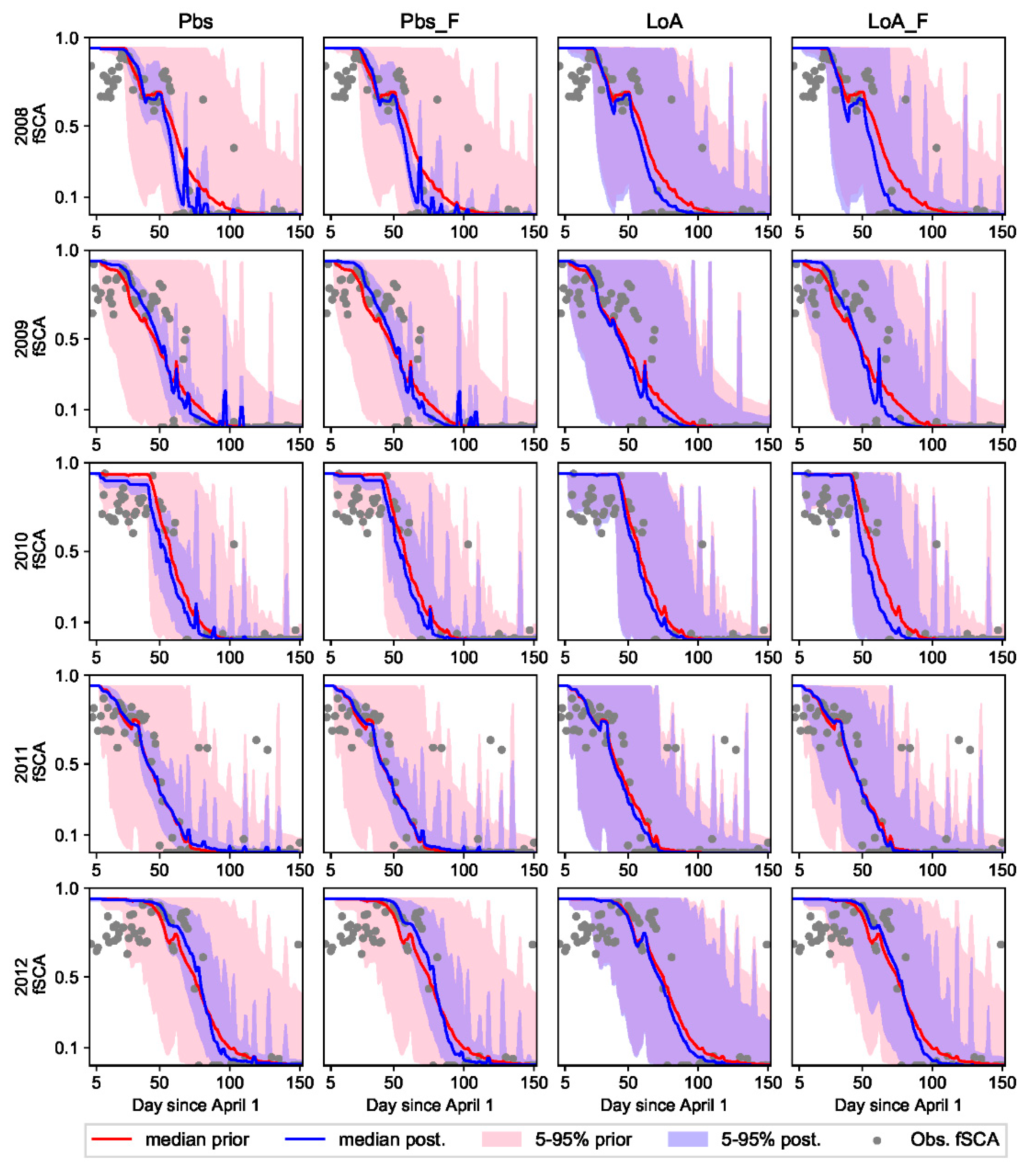
The relative performance of Pbs and LoA varied in response to various factors. LoA was generally more resistant to uncertainties in the assimilated data. When using low quality fSCA measurements with several missing observations, the LoA may yield better result than Pbs. For example, LoA was able to yield relatively better result as compared to the prior estimates in years 2010 and 2015 where there was an overall low performance of the DA schemes in general and Pbs in particular (
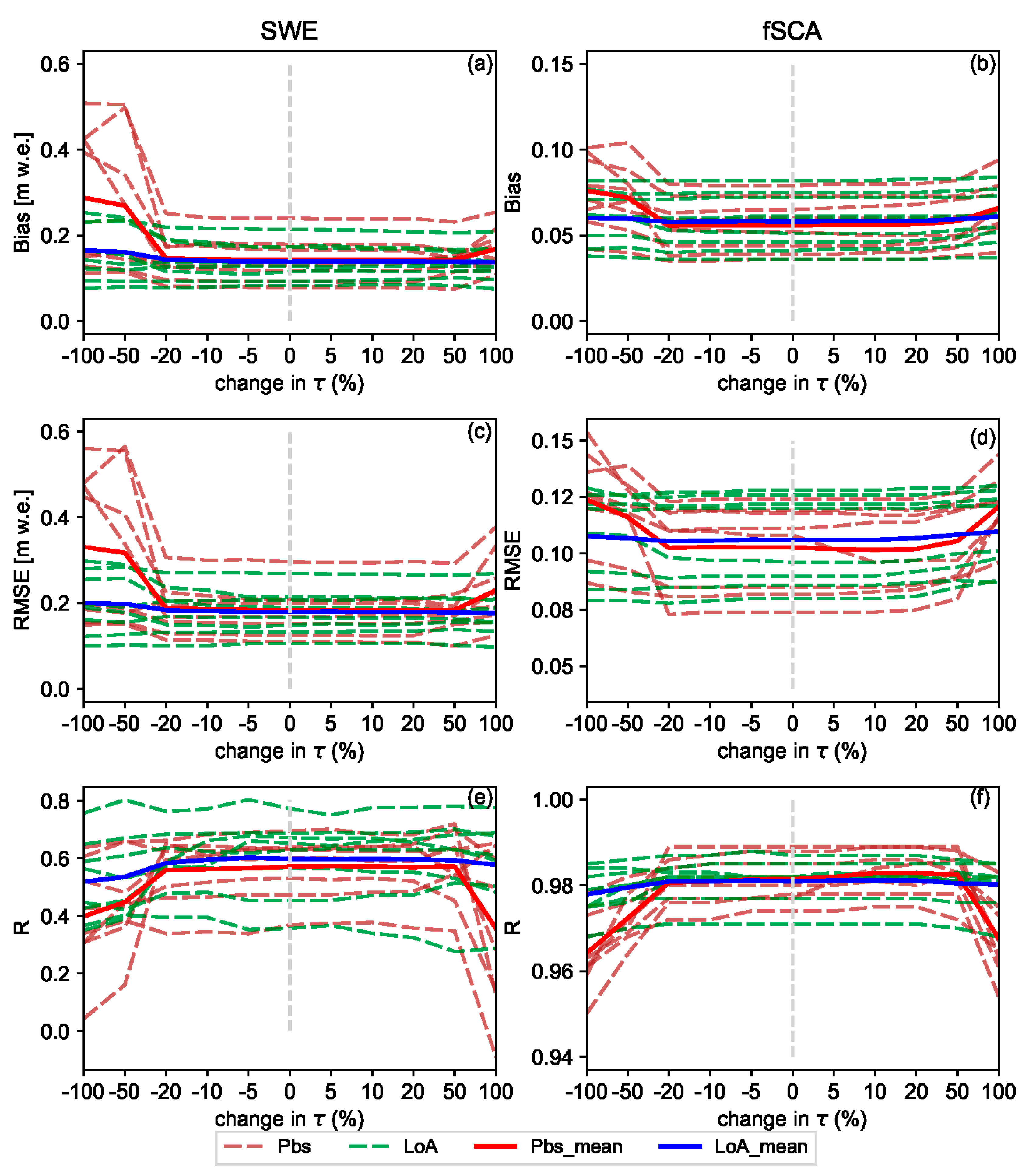
Figure 4). The sensitivity test shown in
Figure 9 also reveals that the Pbs performance gets easily deteriorated as compared to the LoA due to the displacement of the timing window with highest coefficient (W-2) following the changes in location of
. A further advantage of the LoA is that different intuitive evaluation criteria including hydrologic signatures can easily be accommodated in constraining model states and parameters. For example, the overall grade and persistency of an ensemble member in reproducing the observed fSCA within the assumed measurement error bounds are included as evaluation criteria in this study. However, in the presence of several correlated observations such as the fSCA observations from the complete melt-out period, LoA may suffer from identifiability problem to distinguish the best performing ensemble members and this leads to low performance as compared to Pbs. On the other hand, the likelihood with the product of squared residuals renders Pbs a better capability in identifying the optimal ensemble members under such circumstances.
The overall low performance of the DA schemes in years 2010 and 2015 can be attributed to different factors. Following year 2014, these years have lowest observed mean catchment SWE value of 419 and 458 mm respectively as compared to the other years. However, these values are not too far from the average annual value of 525 mm to explain the relatively poor performance of the DA schemes in these years. The total number of fSCA observations in these years and distribution of the observations in the time axis were also assessed since they are expected to have an effect on the DA result. Similarly, no significant difference on the number and distribution of the observations was noticed as compared to the other years. Future studies may thus assess quality of the assimilated MODIS fSCA observations and climatic inputs in relation to the other years since such factors are also expected to play an important role in the DA result.
A fuzzy coefficient was introduced into the original formulations of the two DA schemes in order to take into account for the difference in informational value of fSCA measurements from different timing windows in the ablation period. An fSCA observation in a given time index can assume different informational value depending on its location in the time axis in relation to the critical points. In Pbs and other schemes with square of errors-based likelihood function, value of the efficiency criteria is biased towards data with highest uncertainty, with the bias proportional to the uncertainty squared [
30]. The fuzzy coefficient was thus introduced to rescale the level of this uncertainty with due consideration to the assumed informational value of each observation. The fSCA observations from the more informative period were promoted by allocating higher importance weight, while observations from the other periods were punished in accordance to their location within their respective timing windows. A further assumption in this study was that all observations carry some informational value; albeit to varying degree.
The informational value of fSCA observations with time was assumed to follow an exponential-trapezoidal membership function that broadly divides the ablation period into three timing windows. In W-1, the fSCA measurements close to the onset of snowmelt are generally characterized by low signal to noise ratio. Similarly, during the complete melt-out period (W-3) the measurements are homogenous; and the informational value generally decreases with correlated data that leads to less power in constraining model states and parameters. The critical points of the timing windows, i.e.,
and start of the melt-out period, vary both spatially and temporally in response to various climatic and physiographic factors. This has highlighted the need for a flexible and automatic detection of the critical points. Both the parametric and nonparametric change point detection schemes used in this study yielded similar results with well characterization of the changes. A change point analysis conducted on the transformed data (running total) was found to be more powerful and robust to outliers than the one conducted on the raw data. This can be attributed to the smoothing effect of the noises in the former case. Studies dealing with critical point detection such as the timing of snowmelt onset are also crucial to a better estimate of the surface energy balance in high latitudes, since the fraction of available solar radiation that is actually absorbed almost quadruple during the onset of snowmelt [
3].
The results obtained in this study through assimilation of fSCA into a hydrologic model could also be extended to land surface models (LSMs). Inaccuracies in snow estimates within LSMs can lead to substantial errors in simulation results since snow cover has a significant impact on the surface radiation budget as well as turbulent energy fluxes to the atmosphere [
69]. An assimilation of fSCA into LSMs was reported to improve the simulation result as compared to an open-loop model without assimilation [
69,
70]. Thus, the fuzzy logic-based DA concept presented in this study can also be applied in the assimilation of fSCA, or other variables that display fuzzy informational value with time, into LSMs in order to get an improved result. Alternatively, the use of these schemes could indirectly yield an improvement in the performances of LSMs through improvement in the hydrologic component when LSMs are coupled with the latter. In recent years, there has been growing interest in incorporating a hydrologic component into land surface models (LSMs) in order to improve weather and extreme hydrologic condition forecasts [
71,
72].
Generally an improved estimate of SWE was observed as a result of reanalysis using the DA schemes with a fuzzy coefficient, although, a slight deterioration in some of the evaluation metrics of fSCA was observed when using Pbs_F. This can be attributed to the relatively lower weight assigned to observations from start of the melting period coupled with the fact that most of the weights are carried only by few ensemble members. During the onset of snowmelt, sensitivity of the SDC to the initial bare ground fraction is highest and updates during this period are more likely to be dominated by this parameter than the snow coefficient of variation or precipitation [
52]. The increase in fSCA error was, however, very small as compared to the improvement attained in SWE estimate. Results from this study suggest that, the concept of variable informational value of fSCA observations is consistent with the notion that many of the variables that we usually consider to be crisp quantity and deterministic are actually fuzzy that carry considerable amount of uncertainty [
64].
5. Conclusions
Two ensemble-based data assimilation schemes, i.e. particle batch smoother (Pbs) and the limits of acceptability (LoA) as well as newly introduced versions of these schemes that account for the variability in informational value of the assimilated observation (fraction of snow cover area, fSCA), i.e., Pbs_F and LoA_F, were used to reanalyze the model results. Using the LoA approach as a DA scheme yielded a promising result. All DA schemes resulted in a posterior snow water equivalent (SWE) estimate that is better than the prior estimate in terms of accuracy as measured using one or more of the efficiency criteria used in this study. The result was generally encouraging given the high level of uncertainty associated with optical remote sensing data in general, and MODIS fSCA product in particular in high latitude areas.
Although all fSCA observations in the ablation period were important in constraining the perturbation parameters, some observations were more important than others depending on their location in the time axis with respect to certain critical points in the melt season, i.e., the points where the mean snow cover changes () and the start of a melt-out period. These critical points varied from year to year and spatially between the grid cells. The parametric (likelihood-based) and non-parametric change point detection schemes employed to locate in each grid cell and year yielded reasonable results. A fuzzy coefficient was introduced in the original formulations of Pbs and LoA that renders highest importance weight to the assumed most informative timing window, i.e., to observations between these critical points. A sensitivity test conducted by moving the fuzzy coefficient value assigned to this timing window forward and backward in the time axis revealed that, although somewhat insensitive up to certain distance from its original location, moving this window farther lead to deterioration of the DA results.
The reanalyzed SWE using Pbs_F was superior to Pbs throughout all years, although the degree of improvement in the evaluation metrics varied from year to year. Similarly, an improved estimate of fSCA was obtained for all years when using LoA_F as compared to LoA. On the other hand, the improvement in SWE estimate when using LoA_F in comparison to LoA as measured using a given efficiency criterion was not consistent throughout the analyses years. In many of the analysis years, the relative performance of the DA schemes was also variable from one site to another. Future studies can examine the physiographic and climatic factors affecting the relative performance of these DA schemes in order to get a better insight into the relationship between the underlying concept of the DA schemes and these factors.
Generally, incorporating the variable informational value of the remote sensing data in the DA schemes was a viable option for an improved estimates of the perturbation parameters and thereby the reanalyzed SWE values. The assumed informational values of the fSCA observations with respect to their location in the time axis was based on the general concept that observations with high uncertainty are more likely to have more informational value than certain observations. Future studies can be focused on assessment of the informational values using the well-established techniques based on the information theory and statistical measures. Although this study was focused on fSCA assimilation, the fuzzy logic-based ensemble frameworks presented in this study can be applied to assimilation of other measurements that display variable informational value with time.


