ENSO and Teleconnections Observed Using MISR Cloud Height Anomalies

Abstract

Cloud-top height is an important climate variable due to its greenhouse effect, as well as being a useful indicator of circulation patterns. We use effective height anomalies from stereo retrievals at a horizontal resolution of 1.1 km after subtracting regional and seasonal mean values. After 18 years, any trend in the global average height anomaly remains hidden by the stronger influence of intermittent El Niño–Southern Oscillation (ENSO) events. However, interesting teleconnections and oscillatory patterns in regional cloud heights are starting to emerge. Different teleconnection patterns are now evident during the El Niño and La Niña phases giving rise to high values of the correlation coefficient between many global regions and the Central Pacific, which shows the greatest connection to ENSO. Cloud heights over the Central Pacific and Maritime Continent oscillate out of phase with each other and have nearly synchronous zero anomalies with a mean separation of about 1.8 years. These are lagged by one month from similar zero values in the Southern Oscillation Index. Surface zonal wind anomalies for these two regions also oscillate out of phase with each other, and are highly correlated with the height anomalies, leading them by one month.

1. Introduction

The importance of cloud heights to global climate was noted at least 40 years ago with the realization that a rise of 600 m in the effective cloud-top height would, in isolation, increase equilibrium surface temperature by 2 K [1]. From Davies and Molloy [2], the effective height, H, refers to the integral of the probability distribution of finding a cloud-top in a given altitude range, weighted by altitude. That is,

$$H={\displaystyle \underset{0}{\overset{\infty }{\int }}hf(h)dh}$$

(1)

where $f(h)dh$ is the probability of cloud-top occurrence with height between h and h+dh. Consistent with Davies and Molloy [2], the integral includes the clear sky case when h is the height of the surface above mean sea level. Instantaneous cloud heights observed by the Multi-angle Imaging SpectroRadiometer (MISR) on a horizontal scale of ≈1 km have a standard deviation of ≈2 km when sampled globally. The precision with which H is measured thus depends strongly on the ability to sufficiently sample the height distribution.

The large natural range of cloud-top heights also places strong constraints on the interpretation of observed changes in effective height, especially if this involves databases from different instruments. Cloud height databases, as summarized by Stubenrauch et al. [3], fall into two general classes—radiometric and geometric. Radiometric cloud heights are sensitive to instrument calibration as well as to the choice of ancillary data used to infer altitude [4]. Geometric cloud height databases, such as from the Cloud-Aerosol Lidar with Orthogonal Polarization (CALIOP) [5] and MISR [6], avoid the need for ancillary data, but can have different sensitivities to the detection of thin cloud. Ideally, cloud-top height changes are best studied using a uniform time series from a single instrument, or from essentially identical instruments. An additional consideration due to the large natural range of H is to first remove the long-term seasonal and regional average $\overline{H}$ and to then work only with the height anomalies, $H^{\prime }=H-\overline{H}$. Given a uniform time series from a stable satellite sensor, the precision with which $H^{\prime }$ is obtained depends directly on the number of independent samples.

While time series of global cloud height anomalies are of direct interest to studying global climate change, the length of current records is still too short to identify any significant trend in response to global warming. In a recent paper, Davies et al. [7] used the longest available time series of geometrically measured cloud heights to note that perturbations by El Niño–Southern Oscillation (ENSO) events dominated the 15-year time series of global cloud height anomalies from MISR, but that there appeared to be interesting regional variations associated with these perturbations.

In addition to their global significance, variations in cloud heights provide visual clues to teleconnection patterns that may supplement traditional approaches based on sea surface temperature, winds, precipitation or 500 hPa heights. In this regard, they are analogous to anomalies in outgoing longwave radiation (OLR), which were shown by Chiodi and Harrison [8] to provide a useful perspective on ENSO events. The merits in using MISR cloud height anomalies are: that they are relatively independent of near surface conditions, being strongly dependent on changes in upper level clouds through Equation (1); that they sample uniformly over latitude and are unaffected by the relative absence of Southern Hemisphere observations that may affect reanalysis products; and that they, being geometric, are not affected by temperature anomalies that also affect OLR.

This paper extends our earlier results [2,7] by over three years, to May 2018. This longer time series now includes the strongest El Niño since the launch of the Terra satellite in December 1999 and motivates us to examine the regional behavior of cloud heights in greater depth. There are now sufficient data to extract different subsets in global teleconnection patterns that are related to ENSO. The connection between ENSO and cloud heights is also very strong in certain equatorial regions, and we can relate the observed oscillatory behavior in these cloud heights to changes in the Southern Oscillation Index with high confidence. We can also identify the relative phase differences between cloud heights, surface wind anomalies, and the Southern Oscillation Index (SOI).

2. Data Sources and Analysis Methods

The MISR cloud heights come from the Level 2 cloud-height product (TC_STEREO version 17), which are based on retrievals at a 1.1 km horizontal resolution across a swath of width about 380 km, extending almost from pole to pole in a sun-synchronous orbit (equatorial crossing at 10:30 a.m. local time). There are 233 distinct orbital paths, broken into 180 “blocks” of length 141 km and effective width of about 380 km. The equator-crossing time of the Terra satellite changed by about 15 minutes over the first two years of the record, creating some artifacts in the results of Davies and Molloy [2]. These artifacts were removed in Davies et al. [7], which discusses the revised sampling and analysis in detail. We used the same approach as [7], but, with the longer time series we changed the baseline used for calculating the long-term means to be from March 2003 to February 2018. This baseline completely exclude the time when the equator crossing changed and is a very conservative approach, given that Davies et al. [7] corrected for the changes in glitter angle. The long-term means were calculated at the path and block level, 26 times a year. That is, each region was specified by its block and path number (≈4 × 10⁴ regions globally), and temporal changes in the annual cycle of mean cloud heights for each region were accounted for by averaging over 14-day increments (the time bins start at March 1 each year, so that the 26th bin contains one or two extra days at the end of February). The subtraction of the regional and time averages yields deseasonalized anomalies that are typically quite noisy and benefit from smoothing using a running mean. The main change from Davies et al. [7] was to make this a 6-month—rather than a 12-month—running mean to give better time resolution when exploring oscillatory behavior.

The Southern Oscillation Index (SOI) used here is that of the Australian Bureau of Meteorology [9]. This is “the standardized anomaly of the Mean Sea Level Pressure difference between Tahiti and Darwin.” These are reported on a monthly basis as the anomaly from the long-term mean for that month, divided by the long-term standard deviation of the pressure difference for that month, and multiplied by 10. Values of SOI > 7 are indicative of La Niña and values of SOI < –7 of El Niño. Between these values, conditions are considered to be neutral.

The surface wind data were taken from ERA-Interim reanalysis data as the daily 10-m zonal winds. These were averaged over the same 26 time bins as the heights and expressed as anomalies by subtracting the long-term mean over the same baseline as the heights. The two regions used were between 3°S and 3°N, from 117°E to 123°E for the Maritime Continent, and 177°E to 177°W for the Central Pacific (the values were not sensitive to the exact dimensions of these regions).

3. Results

3.1. Global Time Series

The time series of global effective height anomalies is shown in Figure 1. As in Davies et al. [7] (Figure 5), the anomalies are averaged uniformly by global area but exclude latitudes poleward of 71.8° to avoid sampling fluctuations in the seasonal illumination of polar regions. The change to a 6-month running mean results in more fluctuations at the start of the time series compared to Davies et al. [7], but otherwise the results are very similar where the time periods agree. The root mean square (rms) interannual fluctuations in annual global height anomaly are ≈17 m, which is greater than the annual sampling error of ≈11 m [7]. Heights have risen slightly over 18 years, but the trend is not significant. This is because the largest anomalies are associated with La Niña (2008, 2011) and El Niño (2016) events. These events clearly affect the global mean anomaly, and the 60 m drop associated with the La Niña in 2008 remains the largest such anomaly. The behavior towards the end of the current time series also appears interesting. The new event of interest occurs during the additional three years when the El Niño rise of 2016 culminates in a sharp drop before rebounding as an even higher anomaly at the end of the record. Clearly, there is more to the global fluctuations than just ENSO perturbations. We await the extension of this series with some interest.

3.2. Teleconnections in MISR Height Anomalies

When regional height anomalies are examined [2,7], it is evident that the amplitudes of some regional anomalies can be far larger than anomalies in the global average, and for many regional areas, these greater amplitudes are not simply a consequence of the reduced sampling. This is especially the case along the equatorial band from 2.9°S to 2.9°N. Davies et al. [7] (Figure 8) showed that the Central Pacific from 160°E to 169°W formed the largest region with coherent height anomalies, followed by the Maritime Continent from 104°E to 133°E. We examined the correlation of height anomalies from all other regions between 60°S and 60°N. To produce images that were a compromise between spatial resolution and noise, we empirically chose a 6-month running mean for each time series, defined the Central Pacific region to lie within (2.5°S–3.6°N, 169°E–176°W), and defined all other regions to be a running mean over 11 consecutive blocks and 13 consecutive paths, or approximately 14°lat by 31°lon. The correlation map for the overall time series is shown in Figure 2. In this and the subsequent two figures, the lighter colors lack statistical significance. Along the Equator this shows the classic dipole between the Central Pacific and Maritime Continent, with secondary centers of positive and negative correlation over the western Indian Ocean and the Atlantic, respectively. The Central Pacific is positively correlated eastward, with regions branching northeast across North America and extending across the Atlantic to Western Europe and North Africa, as well as southeast across the Pacific and continuing around the Southern Ocean with progressively reduced significance, perhaps as far as New Zealand. There is also a strong positive correlation with height anomalies over the Indian Ocean west of 90°E. Negative correlations peak over the Maritime Continent and branch northeast and across the Pacific to about 165°W and southeast across most of Australia to the Southern Ocean as far as 90°W. This generally agrees with the pattern noted by [2] (Figure 3c), but with more data and a change in the relative frequency of positive versus negative SOI values, the average pattern is now more distinct.

The average pattern shown in Figure 2 disguises the variability that occurs in the time series during El Niño and La Niña events. By examining the correlation patterns on a yearly basis, starting in May of each year, we noted that while the majority of years were similar to the average pattern, some were distinctly different, corresponding to La Niña years, and some were stronger, corresponding to El Niño years. The best examples of each are shown in Figure 3 and Figure 4, for La Niña and El Niño, respectively.

During a La Niña year, the Indian Ocean becomes negatively correlated with the Central Pacific, which also extends its influence into the West Pacific. The pattern to the northeast of the Central Pacific also changes significantly.

During an El Niño year, the pattern is similar to the overall average, but some areas of positive correlation have expanded. Note the change to the pattern over much of Australia. The contrast in patterns between 2011 and 2016 is quite striking. The coherence and magnitude of the correlations suggest that there is likely a dynamical explanation for the change in behavior, but it is beyond the scope of this paper to investigate what these may be globally, though in the next section we look more closely at the relative behavior of the Central Pacific and Maritime Continent that is clearly related to the SOI.

3.3. MISR Height Anomalies and the Southern Oscillation Index

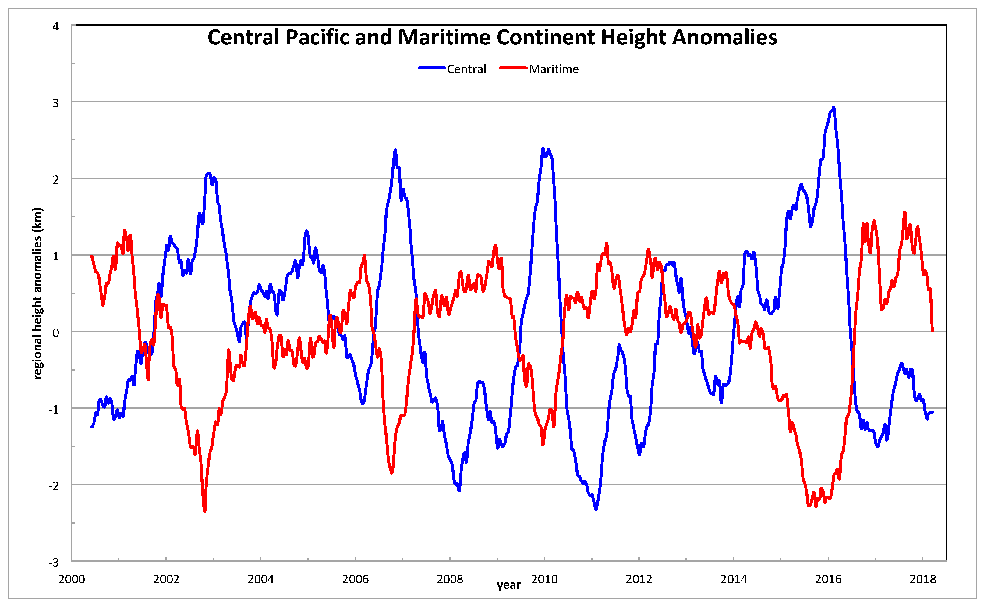
Similar to Davies et al. [7] (Figure 9) but extended by three years and for slightly different regions, Figure 5 shows the complementary oscillation of the Central Pacific and Maritime Continent height anomalies. Here, the Central Pacific region is as described for Figure 2, and the region representing the Maritime Continent is 2.6°S and 2.6°N, 126°E and 134°E (shown as the red rectangle in Figure 2). These regions clearly oscillate out of phase with each other, with peak amplitudes of over 2 km (after 6-month smoothing). The oscillations are closely related to the SOI. In fact, the height anomalies in the two regions can be readily combined to form a height index.

$$\mathrm{HI}=\left(\mathrm{Maritime}\mathrm{Continent}\mathrm{height}\mathrm{anomaly}\right)-\left(\mathrm{Central}\mathrm{Pacific}\mathrm{height}\mathrm{anomaly}\right)$$

(2)

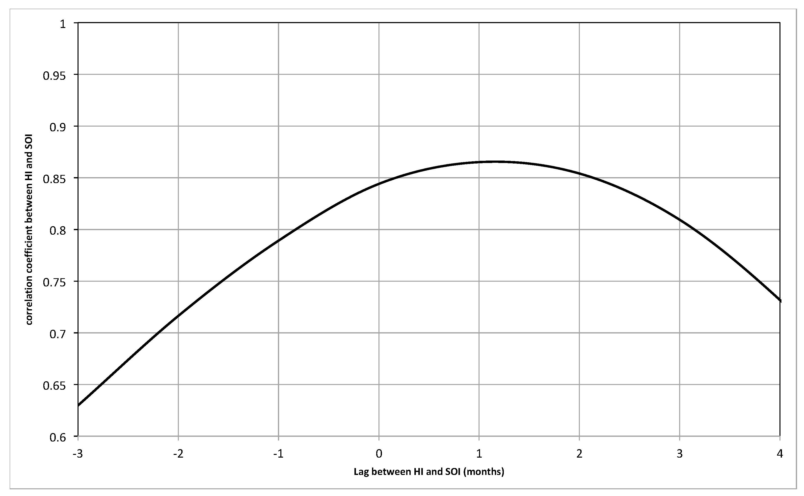
Time series of the Height Indices and the Southern Oscillation Indices are shown in Figure 6. These indices clearly match each other very closely. As defined here, the HI has larger negative values than positive ones because the positive height anomalies are larger for the Central Pacific than for the Maritime Continent, so lacks the relative symmetry of the SOI. We find that HI > 2 km corresponds to La Niña (SOI > 7), and HI < –2 km corresponds to El Niño (SOI < –7). Between these threshold values, the ENSO state is regarded as neutral. While the match between the two indices is very close, with a correlation coefficient of 0.84, this rises to 0.865 when the heights lag the SOI, as shown in Figure 7.

To further explore this lag, we also analyzed the anomalies in the surface zonal winds for the same two regions. Figure 8 compares the height anomalies with anomalies in the near-surface zonal winds, obtained from ERA-Interim reanalysis data [10] over the same time period. The agreement is very good in the Central Pacific. These reach a peak correlation of 0.95, again for a lag of one month. For the Maritime Continent, the presence of land and islands affects the winds somewhat, so that agreement is not quite as good (peak correlation of 0.78 also at a one month lag). The oscillations in wind and effective cloud height are both directly related to ENSO changes, but it appears that the height changes are slightly delayed compared to the winds and to ENSO.

Comparison of Figure 5 and Figure 8 with Figure 6 reveals that the zero crossings of HI and SOI are consistent with the almost synchronous zero anomalies in the regional height and wind anomalies. (In the terminology of statistical physics, the zeros of the HI are degenerate.) As summarized in Figure 9, there are about 10 such zero crossings in the record, with an average separation of 1.8 years. Even though the crossing points have been chosen by inspection, they match the zero anomalies very closely. The 2002 crossing is the least precise, and there is a near-crossing in mid-2011 that we chose to ignore. The SOI has been superimposed on Figure 9 with a one-month lag and inverted to be better comparable with the Central Pacific time series. Despite some differences (there are additional zeros in 2012 and 2015, a delayed zero in 2007, and an earlier zero in 2001) the general agreement between the lagged zeros of the SOI and synchronous zeros of the regional height anomalies gives the impression that the latter are a standard feature of the ENSO system. The regional height anomalies appear to oscillate with a periodicity of about 3.6 years and have an average 1.8-year separation between neutral conditions. The amplitudes of the regional height anomalies vary such that they exceed a threshold of ≈1 km every few oscillations, resulting in $\left|\mathrm{HI}\right|$ > 2 km, coincident with either an El Niño or a La Niña event. Of course, given the one-month lag, the heights are simply a symptom of ENSO behavior, but they may help to characterize it in more detail.

4. Conclusions

We found that remotely sensed cloud heights using MISR’s stereoscopic approach provide a useful tool to analyze climate behavior, both directly on a global basis and indirectly as a clue to circulation patterns through teleconnections and ENSO. On a global basis, we found no significant trend is yet apparent in over 18 years of data. However, large anomalies in the mean global effective height were observed that correspond to El Niño and La Niña events.

The region of the globe with the strongest autocorrelation of height anomalies is located in the Central Pacific. By examining the correlation of other regional height anomalies with the Central Pacific anomalies, we have shown clear teleconnection patterns in height anomalies that stretch around the world (between 60°S and 60°N, Figure 2). These correlation patterns in height bear similarity to earlier studies in cloud cover [11] and OLR [8] and may be a useful indicator for related studies on elongated clouds [12].

By subsetting these teleconnections annually, this paper shows for the first time how such patterns in the correlations of cloud height anomalies differ in individual years, depending on ENSO. The main change from the average pattern occurs during La Niñas, an example of which is shown in Figure 3 for 2011. Here opposite patterns are evident in the western Indian Ocean and much of the Southern Ocean. During a strong El Niño, as shown in Figure 4, the average pattern is mainly reinforced, but with changes over parts of North America and Australia that may be of interest.

This paper also examined the oscillatory pattern between height anomalies in the Central Pacific and the Maritime Continent. As noted in Davies et al. [7], these can be much larger than the global anomalies, and oscillate out of phase with each other (Figure 5). Peak amplitudes of these oscillations, after applying a 6-month smoothing, are between 2 and 3 km. The oscillations were relatively obvious over the 18-year record, defining about 10 fairly clear zero crossings when the Central Pacific and Maritime Continent height anomalies were both zero, resulting in an average separation of about 1.8 years. We have shown in Figure 9 that these zero crossings are closely related to zero crossings in the SOI and zero anomalies in the near surface zonal winds for the same regions. The difference between the height anomalies over the Central Pacific and Maritime Continents provided a robust height index, HI, that matched the Southern Oscillation Index very closely (Figure 6), but with a lag of one month. We are left with the impression that the height oscillations are a routine feature of these regions, and that, once in a while, their amplitudes are large enough to correspond to a recognizable ENSO event. HI greater than 2 km corresponds to La Niña, and less than –2 km to El Niño. The overall cycle, or periodicity, of HI is thus about 3.6 years, on average.

The original intent of this remote sensing paper was to illustrate some of the features present in the stereo-derived cloud heights from MISR over its first 18 years of its operation. However, the connection between height anomalies and ENSO appeared to provide fresh insights to ENSO behavior. The superior sampling of cloud heights at high spatial resolution compared with other currently available techniques allowed a wealth of statistical information to be extracted, supplementing the traditional use of reanalysis data. The convenience of using height anomalies as teleconnection indicators and clues to oscillatory behavior may, it is hoped, encourage further studies, and the MISR time series already appears to be long enough to be useful for such research. For global studies of cloud height feedback in response to global warming, however, it seems that a much longer time series will be needed.

References

- Schneider, S.H. Cloudiness as a global feedback mechanism: The effects on the radiation balance and surface temperature of variations in cloudiness. J. Atmos. Sci. 1972, 29, 1413–1422. [Google Scholar] [CrossRef]
- Davies, R.; Molloy, M. Global cloud height fluctuations measured by MISR on Terra from 2000 to 2010. Geophys. Res. Lett. 2012, 39, L03701. [Google Scholar] [CrossRef]
- Stubenrauch, C.J.; Rossow, W.B.; Kinne, S.; Ackerman, S.; Cesana, G.; Chepfer, H.; Getzewich, B.; Di Girolamo, L.; Guignard, A.; Heidinger, A.; et al. Assessment of global cloud datasets from satellites: Project and database initiated by the GEWEX radiation panel. Bull. Am. Meteorol. Soc. 2013, 94, 1031–1049. [Google Scholar] [CrossRef]
- Stubenrauch, C.J.; Chédin, A.; Armante, R.; Scott, N.A. Clouds as seen by satellite sounders (3I) and imagers (ISCCP). Part I: Evaluation of cloud parameters. J. Clim. 1999, 12, 2189–2213. [Google Scholar] [CrossRef]
- Winker, D.M.; Vaughan, M.A.; Omar, A.H.; Hu, Y.; Powell, K.A.; Liu, Z.; Hunt, W.H.; Young, S.A. Overview of the CALIPSO mission and CALIOP data processing algorithms. J. Atmos. Ocean. Technol. 2009, 26, 2310–2323. [Google Scholar] [CrossRef]
- Moroney, C.; Davies, R.; Muller, J.-P. Operational retrieval of cloud-top heights using MISR data. IEEE Trans. Geosci. Remote Sens. 2002, 40, 1532–1540. [Google Scholar] [CrossRef]
- Davies, R.; Jovanovic, V.M.; Moroney, C.M. Cloud heights measured by MISR from 2000 to 2015. J. Geophys. Res. 2017, 122, 3975–3986. [Google Scholar] [CrossRef]
- Chiodi, A.M.; Harrison, D.E. Global seasonal precipitation anomalies robustly associated with El Niño and La Niña events—An OLR perspective. J. Clim. 2015, 28, 6133–6159. [Google Scholar] [CrossRef]
- Available online: http://www.bom.gov.au/climate/current/soihtm1.shtml (accessed on 25 December 2018).
- Dee, D.P.; Uppala, S.M.; Simmons, A.J.; Berrisford, P.; Poli, P.; Kobayashi, S.; Andrae, U.; Balmaseda, M.A.; Balsamo, G.; Bauer, P.; et al. The ERA-Interim reanalysis: Configuration and performance of the data assimilation system. Q. J. R. Meteorol. Soc. 2011, 137, 553–597. [Google Scholar] [CrossRef]
- Klein, S.A.; Soden, B.J.; Lau, N.-C. Remote Sea Surface Temperature Variations during ENSO: Evidence for a Tropical Atmospheric Bridge. J. Clim. 1999, 12, 917–932. [Google Scholar] [CrossRef] [Green Version]
- Knippertz, P. Tropical–extratropical interactions related to upper-level troughs at low latitudes. Dyn. Atmos. Oceans 2006, 43, 36–62. [Google Scholar] [CrossRef]
Figure 1.
Anomalies in global effective height from MISR from March 2000 to May 2018, smoothed using a 6-month running mean.
Figure 2.
Correlations in effective height anomalies with the Central Pacific from March 2000 to May 2018. The Central Pacific region is defined by the green rectangle between 2.5°S and 3.6°N, and between 169°E and 176°W. Grid lines show latitudes (30°S, 0° and 30°N) and longitudes (90°E, 180° and 90°W). The red rectangle defines the Maritime Continent region used in Section 3.3.
Figure 3.
Similar to Figure 2, but representative of La Niña conditions, from May 2011 to April 2012.
Figure 4.
Similar to Figure 2, but representative of El Niño conditions, from May 2016 to April 2017.
Figure 5.
Time series of regional height anomalies over the Central Pacific and the Maritime Continent from March 2000 to May 2018, smoothed using a 6-month running mean.
Figure 6.
Time series of Southern Oscillation Index (red) and Height Index (black) from March 2000 to May 2018, smoothed using a 6-month running mean. The Height Index, HI, is the difference of the height anomalies in Figure 5 (Maritime Continent–Central Pacific).
Figure 7.
Cross-correlation between Southern Oscillation Index (SOI) and Height Index (HI) as a function of the lag. Positive lag means the HI lags the SOI.
Figure 8.
Similar to Figure 5 for height anomalies (solid lines), with zonal wind anomalies for each region added (dashed lines), both smoothed using a 12-month running mean. CP (blue) refers to Central Pacific, MC (red) refers to Maritime Continent, w (dashed) refers to the wind anomalies, h (solid) refers to the height anomalies.
Figure 9.
Empirically chosen zero crossings (grey) where the Maritime Continent (red) and Central Pacific (blue) height anomalies of Figure 5 are almost synchronously zero. The SOI (black) is plotted with the y-axis inverted and superimposed with a one-month lag, closely matching the Central Pacific height anomalies.
© 2018 by the author. Licensee MDPI, Basel, Switzerland. This article is an open access article distributed under the terms and conditions of the Creative Commons Attribution (CC BY) license (http://creativecommons.org/licenses/by/4.0/).
Share and Cite
MDPI and ACS Style
Davies, R. ENSO and Teleconnections Observed Using MISR Cloud Height Anomalies. Remote Sens. 2019, 11, 32. https://doi.org/10.3390/rs11010032
AMA Style
Davies R. ENSO and Teleconnections Observed Using MISR Cloud Height Anomalies. Remote Sensing. 2019; 11(1):32. https://doi.org/10.3390/rs11010032
Chicago/Turabian StyleDavies, Roger. 2019. "ENSO and Teleconnections Observed Using MISR Cloud Height Anomalies" Remote Sensing 11, no. 1: 32. https://doi.org/10.3390/rs11010032
Note that from the first issue of 2016, this journal uses article numbers instead of page numbers. See further details here.