Crop Classification Based on Temporal Information Using Sentinel-1 SAR Time-Series Data


1
Key Laboratory of Digital Earth Science, Institute of Remote Sensing and Digital Earth, Chinese Academy of Sciences, Beijing 100094, China
2
University of Chinese Academy of Sciences, Beijing 100049, China
*
Author to whom correspondence should be addressed.
Remote Sens. 2019, 11(1), 53; https://doi.org/10.3390/rs11010053
Submission received: 30 November 2018
/
Revised: 20 December 2018
/
Accepted: 25 December 2018
/
Published: 29 December 2018
(This article belongs to the Section Remote Sensing in Agriculture and Vegetation)
Abstract
:With the increasing temporal resolution of space-borne SAR, large amounts of intensity data are now available for continues land observations. Previous researches proved the effectiveness of multitemporal SAR in land classification, but the characterizations of temporal information were still inadequate. In this paper, we proposed a crop classification scheme, which made full use of multitemporal SAR backscattering responses. In this method, the temporal intensity models were established by the K-means clustering method. The intensity vectors were treated as input features, and the mean intensity vectors of cluster centers were regarded as the temporal models. The temporal models summarized the backscatter evolutions of crops and were utilized as the criterion for crop discrimination. The spectral similarity value (SSV) measure was introduced from hyperspectral image processing for temporal model matching. The unlabeled pixel was assigned to the class to which the temporal model with the highest similarity belonged. Two sets of Sentinel-1 SAR time-series data were used to illustrate the effectiveness of the proposed method. The comparison between SSV and other measures demonstrated the superiority of SSV in temporal model matching. Compared with the decision tree (DT) and naive Bayes (NB) classifiers, the proposed method achieved the best overall accuracies in both VH and VV bands. For most crops, it either obtained the best accuracies or achieved comparable accuracies to the best ones, which illustrated the effectiveness of the proposed method.
1. Introduction
Cropland surveillance and land resource allocation are critical to ensure a food supply to feed the global population of over seven billion people. As an all-weather, all-time observation tool, Synthetic Aperture Radar (SAR) is developing rapidly with the recent launches of several space-borne satellites, such as Sentinel-1, Chinese Gaofen-3, and India Risat-1, among others. These satellites are provided with multiple imaging modes, which enlarge the application scope and information content for different demands. With multitemporal or multipolarimetric observations, croplands can be well-characterized through classification [1,2], biological parameter retrieval [3], and phenology monitoring [4,5].
Previous studies of multitemporal cropland classification heavily investigated polarimetric information. For instance, Jiao et al. proposed an object-based classification scheme [6]. Nineteen Radarsat-2 Fine Quad images were used for the experiment. The results with the polarimetric decomposition parameters displayed that the multitemporal data set could acquire high classification accuracies. Whelen et al. utilized the backscattering coefficients and H/A/α decomposition of several L-band UAVSAR data for agricultural classification, and the overall accuracies of the multitemporal error metric method ranged from 75 to 83% [7]. This research noted that the best crop discrimination time should be late spring, late summer or early fall according to a single-year model. Skriver et al. obtained multitemporal C-band and L-band SAR images during a crop-growing season [8]. The classification results of single, dual and fully polarimetric data were compared. The study concluded that multitemporal data were important for single and dual polarimetric SAR classification. In addition, the temporal information might hold a more important status than the polarimetric information. On the other hand, the use of multitemporal intensities alone was also demonstrated to be efficient in crop classification. Skakun et al. combined the multitemporal Radarsat-2 intensity images and the multitemporal Landsat-8 optical data for crop classification with a feed-forward neural network classifier named multilayer perceptron (MLP) [9]. The results showed that the multitemporal SAR intensity data were able to identify winter crops and were helpful in improving summer crop classification results. Kenduiywo et al. developed a classification method with dynamic conditional random fields that combined spatial and temporal information [10]. The method achieved good results, but the spatial interaction model and the temporal interaction model were both embedded in the calculation of random fields, and the crop growth patterns remained invisible.
The above studies either paid more attention to polarimetric information than to the temporal variation of crops or treated multitemporal intensities as independent inputs of machine learning methods. Even though the classifiers, such as SVM [11], RF [12] and DT [13,14], have been demonstrated to be very useful, the backscatter evolution of crops is uninterpretable in these methods. Mindful of this limitation, the intensity variations of multitemporal data are also involved in the classification. Yang et al. considered the temporal variations of backscattering coefficients and introduced the spectral similarity measure (SSM) into the ground classification with manually set thresholds [15]. Whelen et al. presented a case study in North Dakota, USA [16]. The average crop backscattering intensity models were established with repeated trials using different groups of training samples. The classification result was acquired in each trial, and the final result was decided by majority vote. The root mean squared error (RMSE) was applied for the classification, instead of the fixed thresholds applied in his previous work. Murugan et al. designed a knowledge-based classification scheme for harvested and nonharvested sugarcane discrimination [17]. Two criteria were manually set to segment the temporal profiles of the plants. Arias et al. also designed a time-series classification method that used the determination coefficient (R2) and the RMSE as error measures [18].
Those studies explored the effectiveness and potential of multitemporal intensity SAR data in crop classification. However, the methods were either influenced by artificial intervention or by the randomness of a certain model. Thus, in this paper, we propose making a further step with an automatic multitemporal classification scheme with direct descriptions of intensity temporal variations. Compared with the previous studies, this paper contributed in two aspects. First, the automatic temporal model matching method, triggered by the spectral matching techniques of hyperspectral image processing, was designed, which discriminated among crops with their unique backscattering changes. Since the choice of distance measure was not explained in any of the previous studies, in this paper, we demonstrated the superiority of the spectral measure that was applied in the proposed method. Second, considering the diversities in crop growth patterns, multiple models were generated for each crop. The classification result of each pixel was determined through the matchings between intensity curve and temporal models. The effectiveness of our method was illustrated through the comparison with other classifiers.
The rest of this paper is organized as follows: Section 2 illustrates the methodology of the proposed method; Section 3 demonstrates the experimental results and provides brief analyses; Section 4 presents detailed discussions regarding the usability and performance of the proposed method; and finally, Section 5 presents the study’s conclusions.
2. Methodology
In this paper, we proposed a new classification scheme to discriminate different crop cultivation areas with Sentinel-1 data. Multitemporal backscattering coefficients were utilized in this method. For each class, temporal models were generated from multitemporal intensities to characterize the phenology information of the corresponding crop.
Figure 1 gives the flow chart of the proposed method. The method consisted of three steps: data preparation, temporal model generation, and model matching. The preprocessing of the multitemporal SAR data was the data preparation step, which included coregistration, filtering, radiometric calibration and geocoding. The temporal model generation was the second step. In this step, our intent was to find the intrinsic phenology pattern of each class. The K-means clustering method was applied to generate the temporal models of crops. The temporal intensity vector of an N-image sample is taken as the input feature, where xi represents the backscattering coefficients of the ith pixel and N denotes the number of images. The input intensity vector was also regarded as the temporal intensity curve. For each class, several clusters were gathered by the K-means clustering method. Each cluster contained pixels with a similar phenology pattern. The different clusters had slightly different growth patterns, but all belonged to the same class. In addition, the intensity curves of cluster centers were then regarded as the temporal models.
In the final step, temporal model matching was used to realize the classification. The spectral similarity value (SSV) measure was adopted to evaluate the intensity curve similarities between pixel and temporal models [19]. Given an N-dimensional intensity vector and a model center intensity vector , SSV was defined by
where μi and μc denote the means of sample xi and center xc, respectively, and σi and σc represent the standard deviations of sample xi and center xc, respectively. ED is the Euclidean distance, and SCS refers to the spectral correlation similarity. These two measures are also frequently used in hyperspectral curve matching. As a combination of these two measures, SSV characterizes both shape and distance similarities between two spectral curves. In the model matching process, the SSV value was computed between the intensity curves of an unlabeled pixel and each temporal model. The temporal model with the highest similarity was chosen, and the unlabeled pixel was assigned to the class to which this temporal model belonged.
In a single-temporal image, different crops might have similar backscattering responses. However, with multitemporal data, the characterization of the intrinsic crop growth pattern becomes possible. The physical attributes that influence backscattering change continuously with crop growth. These changes are usually distinctive for each crop, because it is unlikely for two crops to have exactly the same temporal variation pattern. The differences between their temporal variation trends are the key to their discrimination. Thus, the idea of temporal model generation is triggered. With reliable temporal models, crop backscattering evolutions can be described directly, and their connections with vegetation biological parameters can be analyzed. However, in reality, the backscattering coefficients of plants are influenced by many factors, such as varieties, plowing directions, and sowing times, among others. These factors often lead to diverse biological and phenological evolutions. As a result, for a certain crop, one temporal model might not be sufficient to interpret the temporal variation comprehensively. Thus, in the proposed method, the K-means clustering was utilized to generate multiple temporal models. The users can set the number of clusters according to their prior knowledge of local agriculture.
Note that the proposed classification method was designed for multitemporal intensity images. The performance of the method is closely related to the number of images. As the image number decreases, the proposed method could lose efficacy. When the number of images decreases to 1, the proposed method becomes a minimum distance classification using a single-temporal intensity image. As a result, the generation of an ideal temporal model requires observation of a complete crop growth cycle.
3. Experimental Results
3.1. Experimental Data and Study Areas
In this paper, two study areas were used to illustrate the effectiveness of the proposed method. The areas had different locations and crop cultivation calendars. Introduced in detail in the following sections are data collection, field research, and local cultivation situations.
3.1.1. Site 1: Wuqing District
The first study site was in the Wuqing district, Tianjin city, China. Nine Sentinel-1 IW mode dual-pol SLC images (VH/VV bands) were acquired from July 2, 2017/Day-of-Year (DOY) 183 to October 6, 2017/DOY 279, as listed in Table 1. The images were observed in the right-looking direction, ascending orbit, and the mid-swath incidence angle was 33.689°. Figure 2a shows the false color composite (FCC) image of the experimental data, where the VH intensities on DOY 207, 231 and 255 represent the RGB channels, respectively. This area belongs to the North China Plain, one of the most important crop-producing regions of northern China. The dominant crop in the study site was summer corn, along with some rice and soybean fields. In addition, the data set covered the full growing seasons of summer corn and soybean. The preprocessing of experimental data was accomplished by Sentinel’s Application Platform (SNAP) software of European Space Agency (ESA), including coregistration, multitemporal filtering, geocoding and radiometric calibration. To acquire accurate knowledge of this area, field studies were carried out to collect ground truth and phenology information of the concerned fields. The ground truth map is shown in Figure 2b, and Figure 3 has some photos of corn in different growth stages. According to the field research, corn accounted for 78.3% of all investigated parcels. Soybean was the second most important crop but only accounted for 8.9% approximately. The amounts of grass and lotus were both approximately 5.7%. Rice only accounted for 1.4%, making rice the most rarely planted crop in this area. The classification accuracies of rice might be influenced by such large differences in cultivation.
3.1.2. Site 2: Fuyu City
The second study site was in Fuyu city, Jilin Province, as shown in Figure 4. Jilin Province is on the Songnen Plain, which is one of China’s major granaries. From May 23, 2017/DOY 143 to October 26, 2017/DOY 299, thirteen Sentinel-1 IW mode dual-pol SLC images (VH/VV bands) were acquired in the left-looking direction, descending orbit. Table 2 gives the data acquisition time. Note that data on DOY 239 are missing because of an observation conflict. The mid-swath incidence angle of the Fuyu area was 39.143°. After image preprocessing, the FCC image of the study area was constructed with VH intensities on DOY 179, 227 and 287, as shown in Figure 4. In this study site, corn was the most common grain in the area, which accounted for approximately 59%. The percentage of peanut, rice, and soybean was approximately 28, 8, and 5%, respectively. The ground truth map was drawn according to the visual interpretation of optical images and prior knowledge of local agriculture. Several parcels were selected according to visual interpretation, as shown in Figure 4. These samples were used for temporal model training and accuracy evaluation.
3.2. Temporal Model Generation
With the observations that covered the full growth cycle of local crops, temporal models were generated for the two study sites. To guarantee sufficient samples for K-means clustering, three thousand pixels were randomly selected for each class. To ensure that the generated temporal models could reflect different growth patterns but meanwhile have little redundancy, the cluster numbers of K-means were tested repeatedly from 1 to 10 for each crop. Table 3 lists the final numbers of the temporal model for each crop type. In general, 5 to 8 clusters were sufficient to basically cover all growth patterns.
Figure 5 and Figure 6 show the temporal models of the two study sites. The multitemporal intensities of clustered centers were plotted, and the green areas denoted the data ranges. In general, VH and VV bands displayed different temporal trends. The backscattering coefficients of the VH band increased as crops germinated and reached the highest levels as plants entered the reproductive stage. When plants entered the maturation stage, the biomass declined because of dehydration, leading to decreases in backscattering coefficients as well. Finally, the intensities sharply decreased after harvest. In contrast, the variations of the VV band presented diverse temporal trends, especially for corn, soybean, and rice. The reason was that the VV band suffered from the complex effects of changes in the scattering mechanism. The developments of stem and leaf changed the dominant scattering mechanism from surface scattering into double-bounce scattering or volume scattering. Moreover, these influences on the VV band also varied with crop type. Note that even though the two study sites both cultivated corn, soybean, and rice, the temporal models of these crops were quite different in the two study sites, especially for corn and rice in the VV band. The reasons were manifold. First, the data acquisition conditions were different: the numbers of images and the image collection times were different, which made the matching of intensity curves difficult and inaccurate. Moreover, the climate differences of the different locations influenced cultivation practices, which caused discrepant backscattering features even for the same crop. Moreover, the backscattering signals were also influenced by the observation geometry. As a result, the different temporal models for these two study sites were quite reasonable.
3.3. Comparison of Similarity Measure
The proposed method extracted the temporal intensity vector from the time-series data and regarded the intensity vector as the intensity curve. The establishment of a temporal model makes the interpretation of the backscatter change during crop growth possible. If the intensity curve of an unlabeled pixel is very similar to that of a temporal model, then the pixel is assigned to the class to which the temporal model belongs. Since the input feature of this process is the intensity curve, the intrinsic nature of the classification is the similarity evaluation between curves, which leads us to the idea of spectral matching techniques.
Many measures evaluate spectral curve similarity from different aspects. In previous studies, the SSV measure was introduced in SAR analysis [11], but whether this measure was superior to other measures was never discussed. Thus, in this section, to demonstrate the effectiveness of SSV, we compared the accuracies of SSV and other spectral matching measures using Site 1. As components of SSV, the distance measure ED and the shape measure SCS were involved in the comparison. Moreover, the spectral angle measure (SAM) and the spectral information divergence measure (SID) [20,21] were also taken into the comparison because of their wide utilization in the hyperspectral image process. As defined in equations (3) to (5), SAM portrays the angle between two spectral vectors, and SID evaluates the probability distribution differences between two spectral vectors:
where and indicate the probability vectors of sample xi and center xc, respectively. Among these measures, SSV, ED, SAM, and SID characterize the difference between two spectral curves so that higher values indicate higher discrepancies; SCS represents the similarity between two curves so that a higher value indicates a higher resemblance. Table 4 gives the classification accuracies of the different measures, and the performances were evaluated by user’s accuracy (UA), producer’s accuracy (PA), overall accuracy (OA) and the kappa coefficient (KA).
As reflected by Table 4, the SSV clearly achieved superior OAs and KAs in the VH and VV bands. The ED measure achieved similar results to those of SSV, so this measure could be taken as an alternate strategy. The SCS measure obtained the lowest OAs and KAs and some very low UAs and PAs. These results indicated that the distance measure might be more important than the shape measure in the curve matching process; the shape measure alone might not be sufficient for temporal model matching. The probability-based measure SID achieved comparable performances to those of SAM. These two measures performed worse in the VV band than in the VH band, especially for corn and grass.
Compared with the VV band, the VH band achieved significantly better OAs because the VH band contained more volume scattering information than that of the VV band. Compared with those of the VH band, the OAs of SSV and ED measures only decreased by 2.30 and 2.35%, respectively, in the VV band. However, for the other three measures, SCS, SAM and SID, the OAs decreased by 16.37, 14.33, and 14.15%, respectively. These results highlighted that a proper similarity measure could ensure good classification performances of the VV band, leading to results comparable to those of the VH band.
A high PA indicates a low omission rate. In both VH and VV bands, the SSV acquired the highest PAs of corn and lotus. In the VH band, soybean was best discriminated with SAM and SID, but the highest PA was only 4.88% higher than that of SSV. Compared with those of SAM and SID, the PAs of rice and grass were approximately 10 and 6% lower, respectively, in the SSV results. However, in the VV band, the SSV achieved the highest PAs of rice and grass, which surpassed those of SAM and SID by approximately 5 and 11%, respectively.
A high UA denotes a low commission rate. The UA can be influenced by sample sizes. Since corn was the dominant grain in Site 1, the commission pixels from other classes composed only a small percentage among all classified corn pixels, which led to high UAs in all measures. The VH band also performed slightly better than the VV band, because the VH band characterized the volume scattering mechanism more properly. However, for the other crops, the commission pixels from corn affected the UAs severely. In the VH band, the UAs of corn, soybean, and grass were similar for all measures. The UAs of lotus in the SSV and ED results were approximately 15% higher than those in the SCS, SAM, and SID results. However, SSV and ED obtained much lower UAs of rice because of the misclassified corn and soybean pixels. In the VV band, the UAs of soybean, grass, and lotus in the SSV and ED results were obviously higher than those of the others. Compared with the VH band, the UAs of rice in the VV band largely increased for SSV and ED and were only 2% lower than the highest one. These results might be related to the double-bounce scattering effects between stems and water surface, which made rice more distinctive and reduced the misclassified pixels from corn and soybean. For a similar reason, lotus also obtained better UAs in the VV band, except for the case of SCS. Compared with the VH band, the UAs of grass were much lower in the VV band, because the VV band was strongly influenced by the surface scattering mechanism, which added difficulties to grass discrimination. However, under such a circumstance, SSV and ED still achieved better UAs than those of the other measures.
3.4. Comparison with Other Classifiers
To illustrate the effectiveness and robustness of the proposed temporal model matching method, we compared its classification results with those of two classic and widely used classification algorithms: decision tree (DT) and naive Bayes (NB) classifiers. The same training samples that generated the temporal models were used in the DT and NB classifiers. The DT classifier is one of the most commonly used machine learning methods for multifeature classification. In this paper, equal weights were set to the input features. The NB method is based on the maximum likelihood estimation. In the experiments, the Gaussian distribution was assumed for the independent input features. The prior probabilities were computed from the frequencies of the training samples. The classification results of the proposed method and the two classic methods were compared qualitatively and quantitatively.
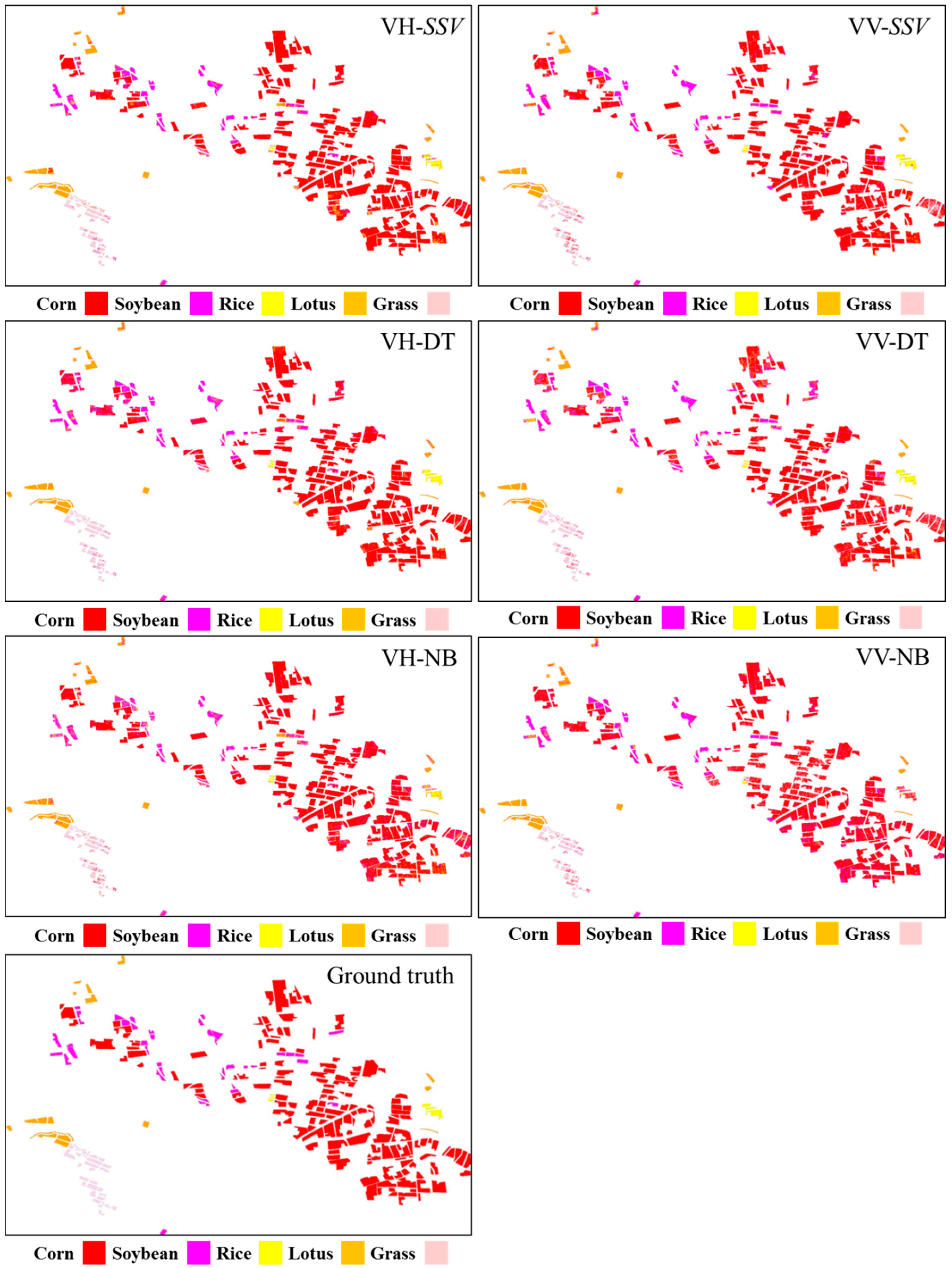
Figure 7 and Figure 8 display the classification maps of the two study sites. The ground truth map of Site 1 and the FCC image of Site 2 were used for the qualitative evaluation. According to visual interpretations of Figure 7, the results of the three methods were very similar, and thus, the proposed method obtained results comparable to those of the other two classifiers. The performance of the proposed method was slightly better with corn mapping, especially in the VV band. In the VV band, the performance of DT was slightly better than that of the other two methods in the detection of lotus. The proposed method and the DT classifier both outperformed NB in rice discrimination.
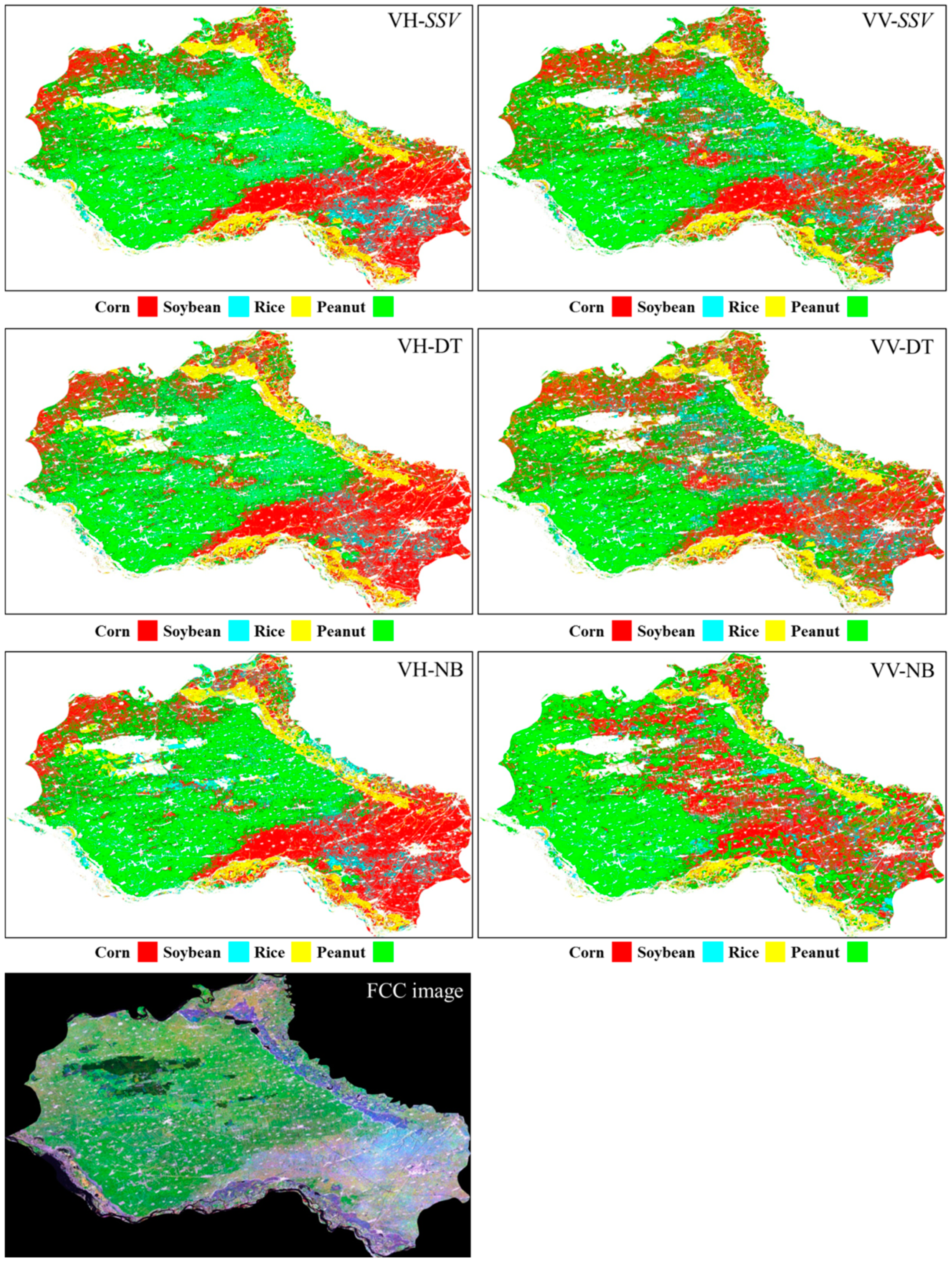
Because of the difficulty in obtaining ground truth data, the intensity of the FCC image in Figure 4 was adopted for the qualitative evaluation of Site 2. As shown in Figure 8, the soybean regions located in the right-bottom part of the image were better recognized by the proposed method than the other two methods. The small area at the image center was mainly cultivated corn, but all methods misclassified this region as peanut in VH band results. The limited numbers of training samples and the complex cultivation practices might have caused this misclassification. However, in general, the VH band classification results of the three methods were in good accordance. In the VV band, the proposed method and the DT classifier performed the best in detecting corn around the image center, but in the right-bottom area, the misclassifications of peanut increased slightly. On the other hand, the NB method wrongly assigned the corn samples at the upper-left corner as peanut and also misrecognized the soybean samples as corn at the right-bottom area and in the center part of the image.
In addition to qualitative comparisons, quantitative evaluations were also made to illustrate the effectiveness of the proposed method. The classification accuracies of the two study sites were evaluated according to the ground truth map in Figure 2b and the labeled samples in Figure 4. Table 5 and Table 6 list the accuracies of the two sites, respectively. In addition, the highest accuracies are noted in bold font. In general, Table 5 and Table 6 reflect similar trends in the qualitative evaluation, and the proposed method achieved good results in the two study sites.
In Site 1, the proposed method achieved the best OAs and KAs in both VH and VV bands and surpassed the NB classifier in all accuracies of all crops. In the VH band, the proposed method achieved the highest PAs of corn and soybean, which demonstrated the effectiveness of the generated temporal model. The PAs of grass and lotus were slightly lower than those of the DT classifier, but the UAs of these two crops were slightly higher than those of the DT and NB methods. The proposed method obtained a higher rice omission rate than that with DT, but the commission rate of rice was similar to that of DT. In the VV band, the proposed method achieved the highest PA of corn and the highest UA of grass and surpassed the NB classifier in all accuracies of corn, soybean, rice, and grass. The UAs of soybean and lotus were comparable to those of the DT method. Although the DT method had the highest PAs of soybean and rice, the method also obtained very low UAs, which indicated severe commission from other classes.
In Site 2, the proposed method acquired OA and KA comparable with those of NB in the VH band and achieved the highest OA and KA in the VV band. In the VH band, the proposed method surpassed the DT classifier in all accuracies and obtained the best accuracies of corn, the highest PAs of soybean and rice, and the highest UAs of rice and peanut. The UA of soybean was lower than that of the NB classifier, because some peanut samples were wrongly recognized as soybean. In the VV band, the proposed method outperformed DT and NB in corn and soybean classification. For rice, the PA of the proposed method was almost the same as that of DT, but the UA was approximately 5% higher than that of the other two methods. The proposed method obtained a lower detection rate of peanut than that with the NB classifier. However, the UA remained the highest. Many corn pixels were misclassified as peanut by NB, leading to the lowest PA of corn, the lowest UA of peanut, and the poorest overall accuracies among the three methods.
4. Discussions
The proposed classification method was composed of two aspects: reliable temporal models and effective model matching strategy. Considering the fluctuations of crop growth patterns, the multiple temporal models were more reasonable than a single model. Thus, to fulfill the requirement for reliable temporal models, the K-means clustering was utilized for temporal model generation. To characterize the variations indicated by the temporal models, the idea of spectral curve matching was introduced. In Section 3.3, different model matching strategies were compared, and the superiority of the SSV value was demonstrated. The results of the ED measure were very close to those of the SSV; thus, it could be taken as an alternate strategy. Through these designs, the availability and effectiveness of the proposed method was determined by data collection and sample selection.
Sufficient multitemporal data and representative training samples are the foundation of reliable temporal models. With a larger number of images, the acquisition of distinctive information is easier; thus, the proposed method required the multitemporal intensity images to cover the crop growth cycle as completely as possible. The selection of training samples requires prior knowledge of the classification area, which can be obtained in many ways, such as field research, optical image reference, and local agriculture investigation. Similar to any other supervised classification method, the training samples should be placed in homogeneous areas and the edges or areas of mixture avoided. Moreover, the temporal models trained in one location can hardly be applied to another location. For instance, the two study sites in this paper both cultivated corn, soybean, and rice. However, the temporal models of Site 1 could not be used for the classification of Site 2. The reason was found in two aspects. First, the image numbers of the two data sets were different. The intensity curves with different lengths should be adjusted before matching, and the classification performances could not be guaranteed. This problem was beyond the concern of this paper but will be investigated in our future research. Second, the backscattering coefficients were also different. Climate differences led to discrepant cultivation practices and backscattering levels of the same crop. For example, in Site 1, the highest VV band backscattering coefficients of soybean were approximately -2 dB. However, in Site 2, the peak value of soybean in the VV band was approximately 3 dB. This type of difference happened many times, which made the temporal models distinct for different locations.
The effectiveness of the proposed method was illustrated by comparison with the DT and NB classifiers. The controlled experiments were carried out on both VH and VV bands with the same training samples. The experimental accuracies directly reflected the abilities of the methods in distinguishing different crops. Compared with the other two methods, the proposed method achieved the highest OAs and KAs in both VH and VV bands of the two study sites. The OAs were all above 90% except the VV band result of Site 1, whose OA was 89.74% and was only 2.3% lower than that of the VH band. In Site 2, the OAs of VH and VV bands were very close and were both approximately 90%. These results illustrated that the proposed method could achieve satisfactory performance in both VH and VV bands. The OAs of the DT method were slightly lower than those of the proposed method but were also close in the two bands, especially in Site 2. However, the cases for the NB classifier were different. In Site 1, the NB classifier achieved comparable OAs in the two bands. However, in Site 2, the OA of the VV band was only 75.52%, which was 14.57% lower than that of the VH band. These results indicated that the performance of the NB method could be influenced by the choice of polarimetric information.
Although the proposed method achieved the best overall accuracies, the method performed differently in different crops. Corn was the dominant crop in the two study sites. The proposed method achieved the best PAs of corn, indicating the best discrimination rates. For the other crops, the proposed method either achieved the best accuracies or obtained comparable results to the best values. In most cases, the differences between the results of the proposed method and the highest accuracies were less than 5%. The exceptions are noted by the gray background in Table 5 and Table 6.
As indicated by Table 5, in the VH band results, the proposed method was slightly inferior to DT in the PAs of grass and lotus and the UA of corn. However, the accuracy differences were no more than 5%, which indicated comparable performances. The only exception was the PA of rice in the VH band. According to the confusion matrix (not shown to save space), more rice samples were misclassified as soybean by the proposed method, so the PA was much lower than that of the DT classifier. However, the UAs of the proposed method and DT were very close and were only approximately 50%, because rice only counted for a small percentage of all crops, and the misclassification from corn and soybean samples severely influenced the UAs. In the VV band, the PA of the proposed method was 93.25%, which was only 4.84% lower than that of DT. Nonetheless, the DT classification results contained many false alarms from corn, which led to a very low UA. As a result, despite that the proposed method was inferior to DT or NB in some accuracies, the differences were small in most cases. This result proved that the proposed method could at least achieve comparable results to those of the widely used classifiers.
According to Table 6, the proposed method achieved the best performances in most cases. However, the proposed method was surpassed by NB in the UA of soybean and the PA of peanut in the VH band results. The comparison between confusion matrixes showed that the proposed method recognized more correct soybean samples but also brought more false alarms from peanut. As a result, the UA of soybean and the PA of peanut were both driven down. In the VV band, the PAs of the proposed method and the NB classifier were 90.14% and 95.78%, respectively, which indicated good discrimination ability for both methods. Compared with NB, some peanut pixels were misclassified as the corn class by the proposed method, which influenced the PA. The NB recognized most peanut samples but also wrongly identified many corn pixels as peanut, so the UA of peanut was only 65.58%, which was much lower than that of the proposed method. Even though NB achieved comparable overall accuracies with the proposed method in the VH band, NB performed much worse in the VV band. Thus, generally, the overall capability of the proposed method still outperformed NB.
5. Conclusions
In this paper, a temporal model matching method was proposed for multitemporal SAR crop classification. The method extracted the temporal variation patterns of the crops under certain observation geometry with the K-means clustering method. The SSV measure was introduced from hyperspectral image analysis to evaluate temporal curve similarities, and the classification was accomplished by the temporal intensity curve matching. Two study sites were utilized to justify the performances of the proposed method. The superior of SSV in temporal model matching was demonstrated for the first time through the comparisons with other spectral measures. The effectiveness of the proposed method was demonstrated by the comparison with the DT and NB classifiers. The proposed method achieved the best overall accuracies, and the performances in the VH and VV bands were comparable. In most cases, the proposed method either achieved the best accuracies or obtained comparable results to the best values.
In the future, temporal models with polarimetric features will be investigated, and the joint model of dual polarimetric SAR intensities will be discussed. Moreover, the generalization of the temporal models will also be discussed. By relating the temporal models to climate factors, such as seed variety, latitude, altitude, irrigation, and temperature, the crop growth details under different circumstances could be characterized. A temporal model library could then be established, which could serve not only the crop classification but also the yield estimation and the market price discovery.
Author Contributions
Conceptualization, L.X. and C.W.; Methodology, L.X.; Softwaer, L.X.; Validation, H.Z. and C.W.; Formal Analysis, L.X.; Investigation, L.X. and C.W.; Resources, B.Z. and M.L.; Data curation, L.X. and B.Z.; Writing-Original Draft Preparation, L.X. and H.Z.; Writing-Review & Editing, L.X. and H.Z.; Visualization, L.X. and H.Z.; Supervision, H.Z.; Project Administration, H.Z.; Funding Acquisition, H.Z. and C.W.
Funding
This research was funded by the National Natural Science Foundation of China under Grants number 41331176, 41371352, and 41371413.
Conflicts of Interest
The authors declare no conflict of interest.
References
- Xie, L.; Zhang, H.; Li, H.; Wang, C. A unified framework for crop classification in southern China using fully polarimetric, dual polarimetric, and compact polarimetric SAR data. Int. J. Remote Sens. 2015, 36, 3798–3818. [Google Scholar] [CrossRef]
- Larranaga, A.; Alvarez-Mozos, J. On the added value of quad-pol data in a multi-temporal crop classification framework based on Radarsat-2 imagery. Remote Sens. 2016, 8, 335. [Google Scholar] [CrossRef]
- Jiao, X.; McNairn, H.; Shang, J.; Pattey, E.; Liu, J.; Champagne, C. The sensitivity of Radarsat-2 polarimetric SAR data to corn and soybean leaf area index. Can. J. Remote Sens. 2011, 37, 69–81. [Google Scholar] [CrossRef]
- Yuzugullu, O.; Erten, E.; Hajnsek, I. Rice growth monitoring by means of x-band co-polar SAR: Feature clustering and BBCH scale. IEEE Geosci. Remote Sens. Lett. 2015, 12, 1218–1222. [Google Scholar] [CrossRef]
- Phan, H.; Toan, T.L.; Bouvet, A.; Nguyen, L.D.; Duy, T.P.; Zribi, M. Mapping of rice varieties and sowing date using x-band SAR data. Sensors 2018, 18, 316. [Google Scholar] [CrossRef] [PubMed]
- Whelen, T.; Siqueira, P. Use of time-series l-band UAVSAR data for the classification of agricultural fields in the San Joaquin valley. Remote Sens. Environ. 2017, 193, 216–224. [Google Scholar] [CrossRef]
- Jiao, X.; Kovacs, J.M.; Shang, J.; McNairn, H.; Walters, D.; Ma, B.; Geng, X. Object-oriented crop mapping and monitoring using multi-temporal polarimetric Radarsat-2 data. ISPRS J. Photogramm. Remote Sens. 2014, 96, 38–46. [Google Scholar] [CrossRef]
- Skriver, H.; Mattia, F.; Satalino, G.; Balenzano, A.; Pauwels, V.R.N.; Verhoest, N.E.C.; Davidson, M. Crop classification using short-revisit multitemporal sar data. IEEE J-STARS 2011, 4, 423–431. [Google Scholar] [CrossRef]
- Skakun, S.; Kussul, N.; Shelestov, A.Y.; Lavreniuk, M.; Kussul, O. Efficiency assessment of multitemporal c-band Radarsat-2 intensity and Landsat-8 surface reflectance satellite imagery for crop classification in Ukraine. IEEE J-STARS 2016, 9, 3712–3719. [Google Scholar] [CrossRef]
- Kenduiywo, B.K.; Bargiel, D.; Soergel, U. Higher order dynamic conditional random fields ensemble for crop type classification in radar images. IEEE Trans. Geosci. Remote Sens. 2017, 55, 4638–4654. [Google Scholar] [CrossRef]
- Shao, Y.; Lunetta, R.S. Comparison of support vector machine, neural network, and cart algorithms for the land-cover classification using limited training data points. ISPRS J. Photogramm. Remote Sens. 2012, 70, 78–87. [Google Scholar] [CrossRef]
- Forkuor, G.; Conrad, C.; Thiel, M.; Ullmann, T.; Zoungrana, E. Integration of optical and synthetic aperture radar imagery for improving crop mapping in northwestern Benin, West Africa. Remote Sens. 2014, 6, 6472–6499. [Google Scholar] [CrossRef]
- McNairn, H.; Champagne, C.; Shang, J.; Holmstrom, D.; Reichert, G. Integration of optical and synthetic aperture radar (sar) imagery for delivering operational annual crop inventories. ISPRS J. Photogramm. Remote Sens. 2009, 64, 434–449. [Google Scholar] [CrossRef]
- McNairn, H.; Kross, A.; Lapen, D.; Caves, R.; Shang, J. Early season monitoring of corn and soybeans with terrasar-x and radarsat-2. Int. J. Appl. Earth Obs. Geoinf. 2014, 28, 252–259. [Google Scholar] [CrossRef]
- Yang, H.J.; Pan, B.; Wu, W.F.; Tai, J.H. Field-based rice classification in Wuhua county through integration of multi-temporal sentinel-1a and Landsat-8 oli data. Int. J. Appl. Earth Obs. Geoinf. 2018, 69, 226–236. [Google Scholar] [CrossRef]
- Whelen, T.; Siqueira, P. Time-series classification of sentinel-1 agricultural data over North Dakota. Remote Sens. Lett. 2018, 9, 411–420. [Google Scholar] [CrossRef]
- Murugan, D.; Singh, D. Development of an approach for monitoring sugarcane harvested and non-harvested conditions using time series Sentinel-1 data. In Proceedings of the International Geoscience and Remote Sensing Symposium (IGARSS), Valencia, Spain, 22–27 July 2018; pp. 5308–5311. [Google Scholar]
- Arias, M.; Campo-Bescós, M.A.; Álvarez-Mozos, J. Crop type mapping based on Sentinel-1 backscatter time series. In Proceedings of the International Geoscience and Remote Sensing Symposium (IGARSS), Valencia, Spain, 22–27 July 2018; pp. 6623–6626. [Google Scholar]
- Thenkaball, P.S.; Teluguntla, P.G.; Biggs, T.; Krishna, M.; Turral, H. Spectral matching techniques to determine historical land-use/land-cover (LULC) and irrigated areas using time-series 0.1-degree AVHRR pathfinder datasets. Photogramm. Eng. Remote Sens. 2007, 73, 1029–1040. [Google Scholar]
- Van der Meer, F. The effectiveness of spectral similarity measures for the analysis of hyperspectral imagery. Int. J. Appl. Earth Obs. Geoinf. 2006, 8, 3–17. [Google Scholar] [CrossRef]
- Hosseini, R.S.; Homayouni, S.; Safari, R. Modified algorithm based on support vector machines for classification of hyperspectral images in a similarity space. J. Appl. Remote Sens. 2012, 6, 063550. [Google Scholar] [CrossRef]
Figure 1.
Flow chart of the proposed method.

Figure 2.
Location and ground truth of Site 1: (a) Location of the Wuqing study site and the FCC image represented by the VH intensities on DOY 207, 231 and 255; (b) The ground truth map of cultivation parcels.
Figure 2.
Location and ground truth of Site 1: (a) Location of the Wuqing study site and the FCC image represented by the VH intensities on DOY 207, 231 and 255; (b) The ground truth map of cultivation parcels.

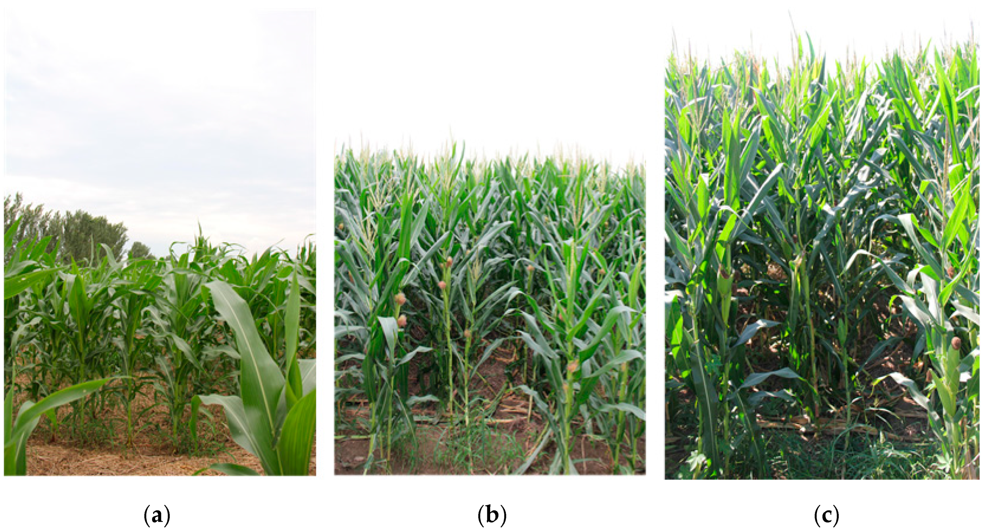
Figure 3.
Photos of corn growth: (a) DOY 207 (jointing stage); (b) DOY 231(jointing stage); (c) DOY 255 (earing stage).
Figure 3.
Photos of corn growth: (a) DOY 207 (jointing stage); (b) DOY 231(jointing stage); (c) DOY 255 (earing stage).

Figure 4.
Location of the Fuyu study site and the distribution of samples, overlaid on the FFC image represented by the VH intensities on DOY 179, 227 and 287.
Figure 4.
Location of the Fuyu study site and the distribution of samples, overlaid on the FFC image represented by the VH intensities on DOY 179, 227 and 287.

Figure 5.
Temporal models of Site 1.

Figure 6.
Temporal models of Site 2.

Figure 7.
Classification results of Site 1: the proposed method and the DT and NB classifiers.

Figure 8.
Classification results of Site 2: the proposed method and the DT and NB classifiers.


Table 1.
Information on the experimental data.
| Acquisition time /Day of year (DOY) | 2017-07-02 /183 | 2017-07-14 /195 | 2017-07-26 /207 | 2017-08-07 /219 | 2017-08-19 /231 |
| Acquisition time /Day of year (DOY) | 2017-08-31 /243 | 2017-09-12 /255 | 2017-09-24 /267 | 2017-10-06 /279 |
Table 2.
Information about the experimental data.
| Acquisition time /Day of year (DOY) | 2017-05-23 /143 | 2017-06-04 /155 | 2017-06-16 /167 | 2017-06-28 /179 | 2017-07-10 /191 |
| Acquisition time /Day of year (DOY) | 2017-07-22 /203 | 2017-08-03 /215 | 2017-08-15 /227 | 2017-09-08 /251 | 2017-09-20 /263 |
| Acquisition time /Day of year (DOY) | 2017-10-02 /275 | 2017-10-14 /287 | 2017-10-26 /299 |
Table 3.
Numbers of temporal models for different crops.
| Site | Site 1: Wuqing | Site 2: Fuyu | |||||||
|---|---|---|---|---|---|---|---|---|---|
| Crops | Corn | Soybean | Rice | Grass | Lotus | Corn | Soybean | Rice | Peanut |
| VH | 7 | 6 | 4 | 3 | 5 | 7 | 10 | 9 | 8 |
| VV | 8 | 5 | 6 | 7 | 7 | 9 | 9 | 8 | 7 |
Table 4.
Classification accuracies with different spectral measures using Site 1 data.
| Band | VH | VV | |||||||||
|---|---|---|---|---|---|---|---|---|---|---|---|
| Class | Corn | Soybean | Rice | Grass | Lotus | Corn | Soybean | Rice | Grass | Lotus | |
| SSV | PA (%) | 93.62 | 78.41 | 85.40 | 92.44 | 92.84 | 90.56 | 80.97 | 93.25 | 89.31 | 91.63 |
| UA (%) | 98.48 | 73.45 | 51.25 | 99.20 | 62.81 | 97.47 | 68.27 | 67.82 | 61.75 | 79.18 | |
| OA (%) | 92.04 | 89.74 | |||||||||
| KA | 0.7998 | 0.7499 | |||||||||
| Class | Corn | Soybean | Rice | Grass | Lotus | Corn | Soybean | Rice | Grass | Lotus | |
| ED | PA (%) | 93.45 | 78.36 | 85.20 | 92.41 | 92.78 | 90.31 | 81.05 | 92.88 | 89.64 | 91.24 |
| UA (%) | 98.47 | 72.62 | 51.05 | 99.15 | 62.64 | 97.49 | 67.55 | 68.41 | 60.63 | 79.57 | |
| OA (%) | 91.89 | 89.54 | |||||||||
| KA | 0.7967 | 0.7459 | |||||||||
| Class | Corn | Soybean | Rice | Grass | Lotus | Corn | Soybean | Rice | Grass | Lotus | |
| SCS | PA (%) | 92.14 | 78.57 | 94.91 | 71.36 | 80.55 | 73.26 | 65.99 | 89.42 | 53.23 | 92.24 |
| UA (%) | 96.77 | 72.97 | 67.01 | 99.66 | 47.05 | 94.89 | 59.84 | 38.64 | 30.12 | 31.69 | |
| OA (%) | 89.17 | 72.80 | |||||||||
| KA | 0.7270 | 0.4568 | |||||||||
| Class | Corn | Soybean | Rice | Grass | Lotus | Corn | Soybean | Rice | Grass | Lotus | |
| SAM | PA (%) | 90.62 | 82.42 | 92.99 | 98.09 | 87.53 | 74.66 | 73.42 | 88.19 | 77.93 | 90.74 |
| UA (%) | 98.60 | 73.14 | 71.32 | 98.69 | 47.31 | 95.52 | 52.64 | 71.05 | 26.65 | 62.37 | |
| OA (%) | 90.16 | 75.83 | |||||||||
| KA | 0.7630 | 0.5107 | |||||||||
| Class | Corn | Soybean | Rice | Grass | Lotus | Corn | Soybean | Rice | Grass | Lotus | |
| SID | PA (%) | 90.74 | 83.29 | 93.63 | 97.99 | 87.97 | 75.15 | 73.92 | 88.60 | 77.69 | 90.77 |
| UA (%) | 98.63 | 72.84 | 72.92 | 98.71 | 48.41 | 95.58 | 53.95 | 68.98 | 26.85 | 62.64 | |
| OA (%) | 90.36 | 76.26 | |||||||||
| KA | 0.7675 | 0.7675 | |||||||||
Table 5.
Classification accuracies of Site 1: comparisons among the proposed method (SSV) and the DT and NB classifiers.
Table 5.
Classification accuracies of Site 1: comparisons among the proposed method (SSV) and the DT and NB classifiers.
| Band | VH | VV | |||||||||
|---|---|---|---|---|---|---|---|---|---|---|---|
| Class | Corn | Soybean | Rice | Grass | Lotus | Corn | Soybean | Rice | Grass | Lotus | |
| SSV | PA (%) | 93.62 | 78.41 | 85.40 | 92.44 | 92.84 | 90.56 | 80.97 | 93.25 | 89.31 | 91.63 |
| UA (%) | 98.48 | 73.45 | 51.25 | 99.20 | 62.81 | 97.47 | 68.27 | 67.82 | 61.75 | 79.18 | |
| OA (%) | 92.04 | 89.74 | |||||||||
| KA | 0.7998 | 0.7499 | |||||||||
| Class | Corn | Soybean | Rice | Grass | Lotus | Corn | Soybean | Rice | Grass | Lotus | |
| DT | PA (%) | 90.25 | 78.03 | 98.49 | 94.34 | 94.76 | 82.08 | 81.06 | 98.09 | 87.28 | 93.56 |
| UA (%) | 98.70 | 60.53 | 51.43 | 97.73 | 61.69 | 98.02 | 52.48 | 27.93 | 57.89 | 74.70 | |
| OA (%) | 89.77 | 83.17 | |||||||||
| KA | 0.7570 | 0.6378 | |||||||||
| Class | Corn | Soybean | Rice | Grass | Lotus | Corn | Soybean | Rice | Grass | Lotus | |
| NB | PA (%) | 86.29 | 64.40 | 79.80 | 86.07 | 91.28 | 83.10 | 70.89 | 26.37 | 86.34 | 92.48 |
| UA (%) | 97.48 | 45.14 | 36.70 | 97.80 | 52.31 | 95.40 | 43.36 | 52.05 | 49.11 | 80.84 | |
| OA (%) | 88.35 | 84.03 | |||||||||
| KA | 0.7743 | 0.7044 | |||||||||
Table 6.
Classification accuracies of Site 2: comparisons among the proposed method (SSV) and the DT and NB classifiers.
Table 6.
Classification accuracies of Site 2: comparisons among the proposed method (SSV) and the DT and NB classifiers.
| Band | VH | VV | |||||||
|---|---|---|---|---|---|---|---|---|---|
| Class | Corn | Soybean | Rice | Peanut | Corn | Soybean | Rice | Peanut | |
| SSV | PA (%) | 94.73 | 85.52 | 97.48 | 82.87 | 88.01 | 97.31 | 90.47 | 90.14 |
| UA (%) | 97.51 | 66.62 | 97.57 | 89.52 | 89.27 | 94.48 | 92.79 | 87.94 | |
| OA (%) | 90.81 | 90.22 | |||||||
| KA | 0.8721 | 0.8626 | |||||||
| Class | Corn | Soybean | Rice | Peanut | Corn | Soybean | Rice | Peanut | |
| DT | PA (%) | 88.49 | 82.65 | 93.68 | 76.41 | 79.74 | 94.90 | 90.95 | 84.90 |
| UA (%) | 93.45 | 59.16 | 89.86 | 86.72 | 85.80 | 85.72 | 87.15 | 83.36 | |
| OA (%) | 85.41 | 85.37 | |||||||
| KA | 0.7980 | 0.7959 | |||||||
| Class | Corn | Soybean | Rice | Peanut | Corn | Soybean | Rice | Peanut | |
| NB | PA (%) | 94.13 | 62.72 | 94.42 | 92.46 | 55.89 | 76.06 | 82.78 | 95.78 |
| UA (%) | 95.30 | 72.48 | 97.19 | 84.79 | 80.14 | 81.26 | 87.21 | 65.58 | |
| OA (%) | 90.09 | 75.52 | |||||||
| KA | 0.8601 | 0.6599 | |||||||
© 2018 by the authors. Licensee MDPI, Basel, Switzerland. This article is an open access article distributed under the terms and conditions of the Creative Commons Attribution (CC BY) license (http://creativecommons.org/licenses/by/4.0/).
Share and Cite
MDPI and ACS Style
Xu, L.; Zhang, H.; Wang, C.; Zhang, B.; Liu, M. Crop Classification Based on Temporal Information Using Sentinel-1 SAR Time-Series Data. Remote Sens. 2019, 11, 53. https://doi.org/10.3390/rs11010053
AMA Style
Xu L, Zhang H, Wang C, Zhang B, Liu M. Crop Classification Based on Temporal Information Using Sentinel-1 SAR Time-Series Data. Remote Sensing. 2019; 11(1):53. https://doi.org/10.3390/rs11010053
Chicago/Turabian StyleXu, Lu, Hong Zhang, Chao Wang, Bo Zhang, and Meng Liu. 2019. "Crop Classification Based on Temporal Information Using Sentinel-1 SAR Time-Series Data" Remote Sensing 11, no. 1: 53. https://doi.org/10.3390/rs11010053
Note that from the first issue of 2016, this journal uses article numbers instead of page numbers. See further details here.