Article

Predictive Ecosystem Mapping of South-Eastern Australian Temperate Forests Using Lidar-Derived Structural Profiles and Species Distribution Models

1
School of Ecosystem and Forest Sciences, Faculty of Science, The University of Melbourne, 500 Yarra Boulevard, Richmond, Victoria 3121, Australia
2
CSIRO Land and Water Business Unit, GPO Box 1700, Canberra 2601, Australia
3
CSIRO Land and Water Business Unit, 15 College Road, Sandy Bay 7005, Australia
4
School of Ecosystem and Forest Sciences, Faculty of Science, The University of Melbourne, 4 Water Street, Creswick 3363, Australia
*
Author to whom correspondence should be addressed.
Remote Sens. 2019, 11(1), 93; https://doi.org/10.3390/rs11010093
Submission received: 30 October 2018 / Revised: 11 December 2018 / Accepted: 11 December 2018 / Published: 7 January 2019
(This article belongs to the Special Issue Advances in Remote Sensing of Forest Structure and Applications)

Abstract

:
Modern approaches to predictive ecosystem mapping (PEM) have not thoroughly explored the use of ‘characteristic’ gradients, which describe vegetation structure (e.g., light detection and ranging (lidar)-derived structural profiles). In this study, we apply a PEM approach by classifying the dominant stand types within the Central Highlands region of south-eastern Australia using both lidar and species distribution models (SDMs). Similarity percentages analysis (SIMPER) was applied to comprehensive floristic surveys to identify five species which best separated stand types. The predicted distributions of these species, modelled using random forests with environmental (i.e., climate, topography) and optical characteristic gradients (Landsat-derived seasonal fractional cover), provided an ecological basis for refining stand type classifications based only on lidar-derived structural profiles. The resulting PEM model represents the first continuous distribution map of stand types across the study region that delineates ecotone stands, which are seral communities comprised of species typical of both rainforest and eucalypt forests. The spatial variability of vegetation structure incorporated into the PEM model suggests that many stand types are not as continuous in cover as represented by current ecological vegetation class distributions that describe the region. Improved PEM models can facilitate sustainable forest management, enhanced forest monitoring, and informed decision making at landscape scales.

Graphical Abstract

1. Introduction

Understanding the composition and structure of forest ecosystems is critical for ecological understanding, and for developing effective forest management strategies. The increased availability of geographic information and remote sensing data for forested ecosystems, in combination with advances in computational modelling, has facilitated the development of predictive ecosystem mapping (PEM) models [1,2,3]. PEM models are defined as methods that identify ecological-landscape relationships from spatial environmental data and field observations (as available) to predict vegetation composition across a landscape [1,2,4,5,6,7]. Using similar approaches but with varying objectives and units, PEM models have been broadly defined as predictive vegetation mapping [1], which also encompass species distribution models (SDMs) [2,3,8,9], bioclimatic envelope models [10,11], habitat suitability or decision-support models [12,13,14], and ecological niche models [15,16]. Such models originated from ecological niche theory whereby vegetation distribution is predicted using variables that either correlate with or define tolerance ranges of species [1,8,9,10,17,18].
There are three typical approaches to modelling community distributions from species and environmental data: (1) assemble species into communities and then predict, (2) predict species individually then assemble into communities, and (3) assemble and predict species together [19,20,21,22,23]. The first approach uses some form of classification, ordination, or aggregation method to generate communities from individual species survey data. The presence-absence locations of each community are then compared with environmental predictors to describe their distributions. The second approach models each species distribution individually as a function of available environmental predictors. A community-level output is then generated from a classification, ordination, or aggregation of all the extrapolated individual species distribution models. The third approach characterizes each community and associated relationships with environmental data in a single process incorporating each species and all environmental data simultaneously. No single approach will be optimal in all circumstances, with the selection dependent on available data and study objectives [21,22]. Ohmann et al. [24] argued that any approach selected should aim to retain information of individual species and patterns of co-occurrence in the final predictions. Joint species distribution modeling (JSDM) is an approach that accounts for both presence-absence and abundance data jointly across species to classify communities [25,26]. Combining independent SDM model outputs may be just as effective as JSDM though where the species of interest do not interact with one another [25]. These techniques all aim to develop predictive models that utilize multidimensional descriptive variables to predict the distribution of vegetation across landscapes.
The use of multiple data types to describe environmental variables and forest structure can result in complex, often non-linear data, which challenges the accuracy of predictive models developed using traditional parametric approaches [27,28,29]. Machine learning techniques have emerged from synergies between computer science and the identification of ecological processes and patterns, known as ecological informatics, which directly address issues of data complexity and non-linearity to generate accurate predictive models [28,29,30]. Some examples of machine learning techniques that have been used for species distribution modelling include artificial neural networks, k-nearest neighbors, support vector machines, boosted regression trees, and random forests [6,8,27,31,32,33,34]. The random forest algorithm, developed by Breiman [35], has two key advantages for forest distribution mapping; (1) the novel variable importance measure, and (2) the proximity measures of similarity among data points [27].
Many predictor variables for PEM models can be measured in the field or collated from various geographic information system layers and remote sensing data [3]. Selection of predictor variables is critical to PEM accuracy [36,37,38,39], with each variable considered in terms of its importance to the distribution of an ecosystem and the ecological basis for its inclusion [18,37]. These variables can include a number of environmental gradients: direct gradients influence growth but are not consumed (i.e., temperature, pH); indirect gradients have a location-dependent correlation with forest distribution but have no functional effect on plant growth (i.e., latitude, altitude, slope); and resource gradients are consumed by vegetation (i.e., light, water) [2,5,18,36]. Interactions between structural and compositional gradients can influence stand development and are important to capture in ecosystem classification [40]. These gradients of structure and composition describe the state of vegetation at a specific point in time (i.e., height, cover, strata), and can be broadly defined as ‘characteristic gradients’. Characteristic gradients are increasingly being included in PEM models with inputs summarizing forest structural complexity into a single metric or multiple metrics when three-dimensional data are available [12,41,42].
Characteristic gradients can be quantified at broad spatial scales using remote sensing compared to spatially limited and cost-intensive field observations. Systematic field observations are often individual locations spread across large areas with limited sensitivity to the vertical assemblage of vegetation. Both horizontal and vertical structure can be obtained across a spatial continuum using light detection and ranging (lidar) technology. Lidar is an active remote sensing technique that uses laser ranging to determine the distance between the sensor and an object. Distance is calculated from half the time-lapse between when the laser pulse is emitted and the detection of the returned pulse after striking an object [14,43,44]. Key sensitivity and accuracy limitations of commonly used optical and radar imagery [45] can be overcome using lidar data [44]. Lidar pulses measure the presence or absence of foliage and topographic structure in three dimensions [46,47,48,49], where optical and radar data responses are generally canopy and mid-canopy driven, respectively [43]. Results from Kane et al. [50] highlight that lidar can accurately characterize forest successional stages in the absence of field measurements. The ability of lidar to exploit small gaps in the forest canopy and capture understorey structure allows for the inclusion of lower strata attributes in predictive vegetation models [51,52,53,54]. Predictive models that include characteristic variables from lidar often use discrete derivatives such as canopy height, foliage cover, leaf area index (LAI), and vegetation density [12,29,50,51,55,56,57,58,59,60]. Recent studies using the vertical continuum of lidar data have typically focused on structure only classifications using random forest [49,61], excluding the use of ecological data pertaining to species composition dominating landscape-scale PEM.
In south-eastern Australia, eucalypt forests have traditionally been delineated based on dominant Eucalyptus species without consideration for associated Acacia, rainforest and understory species [62]. The classification of rainforest focuses on the floristic composition at maturity and excludes changes in species composition over time due to changes in the composition that may be driven by disturbance (i.e., ingress of Acacia and Eucalyptus following fire) [62]. Cameron [62] argued that, while this traditional approach has advantages for interpreting community niche distributions, it is problematic at the ecotones that share dominant species, or where dominant canopy species are replaced by species characteristic of another stand type (e.g., patches of eucalypts within a rainforest mosaic after fire). The potential need to consider both climatic and structural gradients in PEM models for this region was further highlighted in a recent study that indicated both types of variables were important for explaining beta-diversity in the temperate forests of south-eastern Australia [
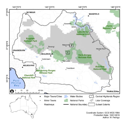
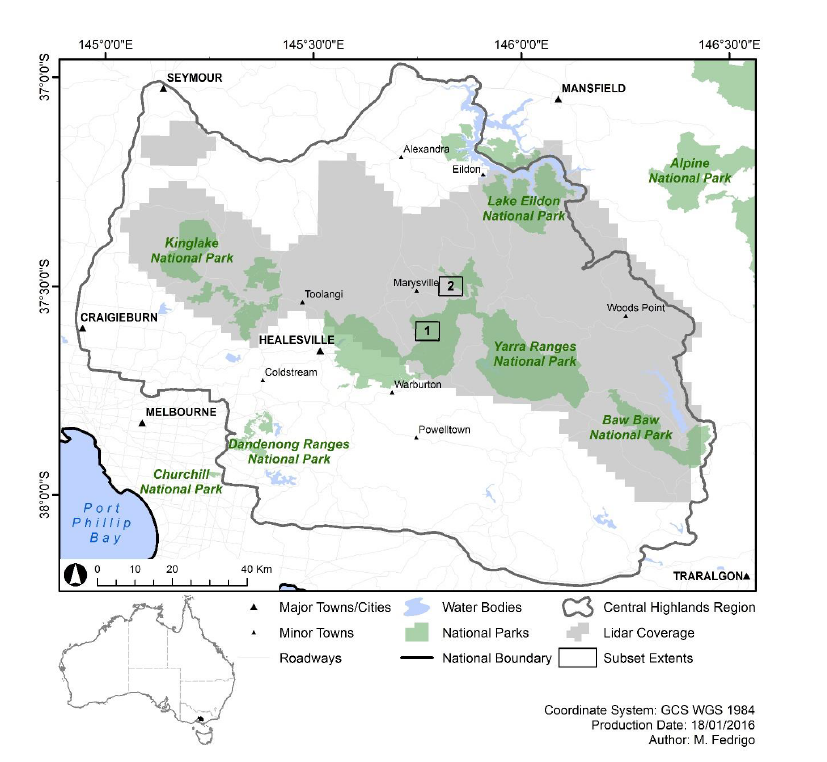
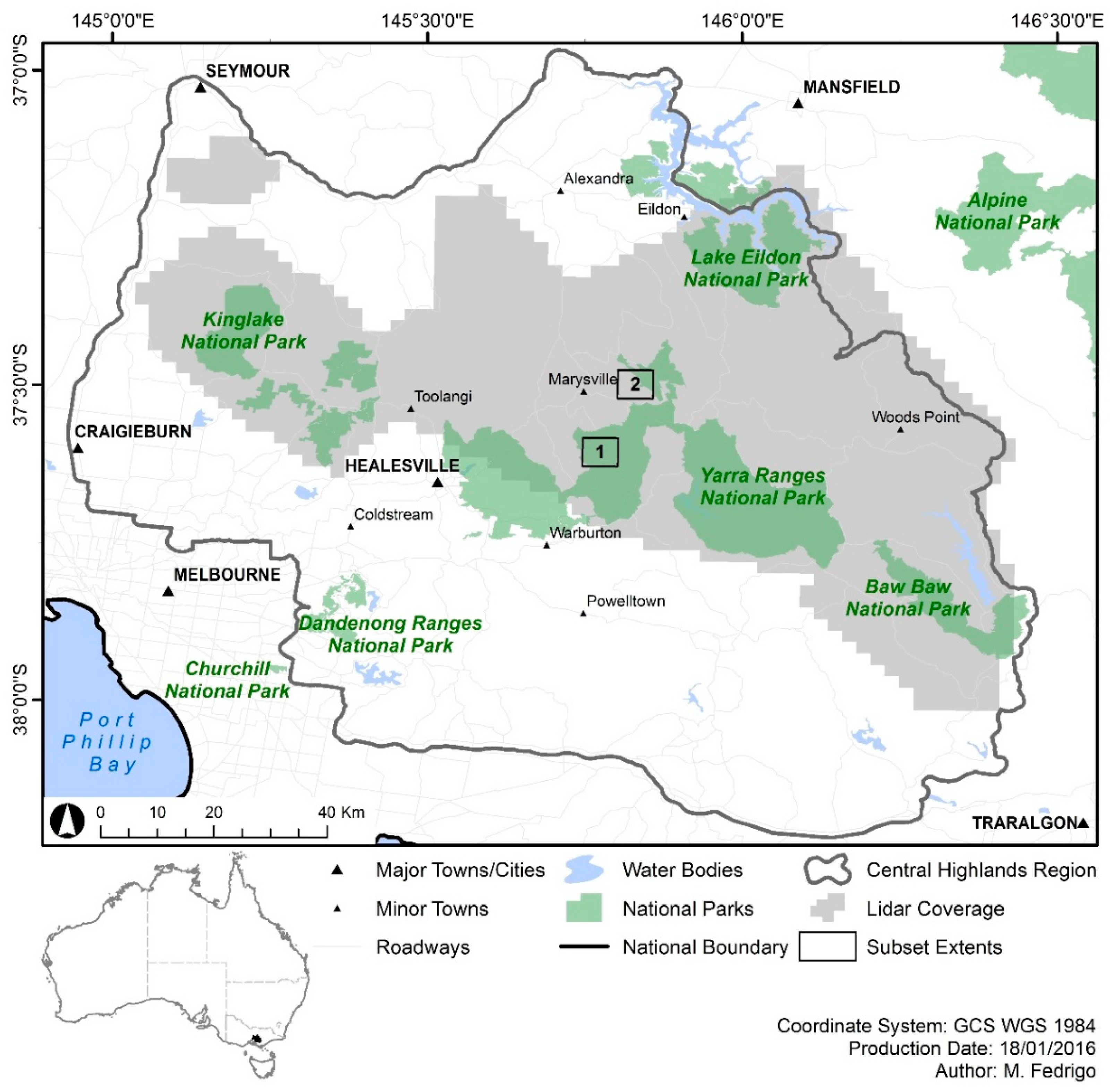
63]. Accordingly, the cool temperature forest landscapes of the Central Highlands region in south-eastern Australia are an ideal case study for examining the potential to improve traditional PEM approaches using structural information such as characteristic gradients. The landscape contains wet sclerophyll forest, rainforest and an ecotone between these two stand types described as ‘cool temperate mixed forest’ [62], which has so far been excluded from the principal vegetation class system in the region (‘Ecological Vegetation Class’, EVC) [64,65].
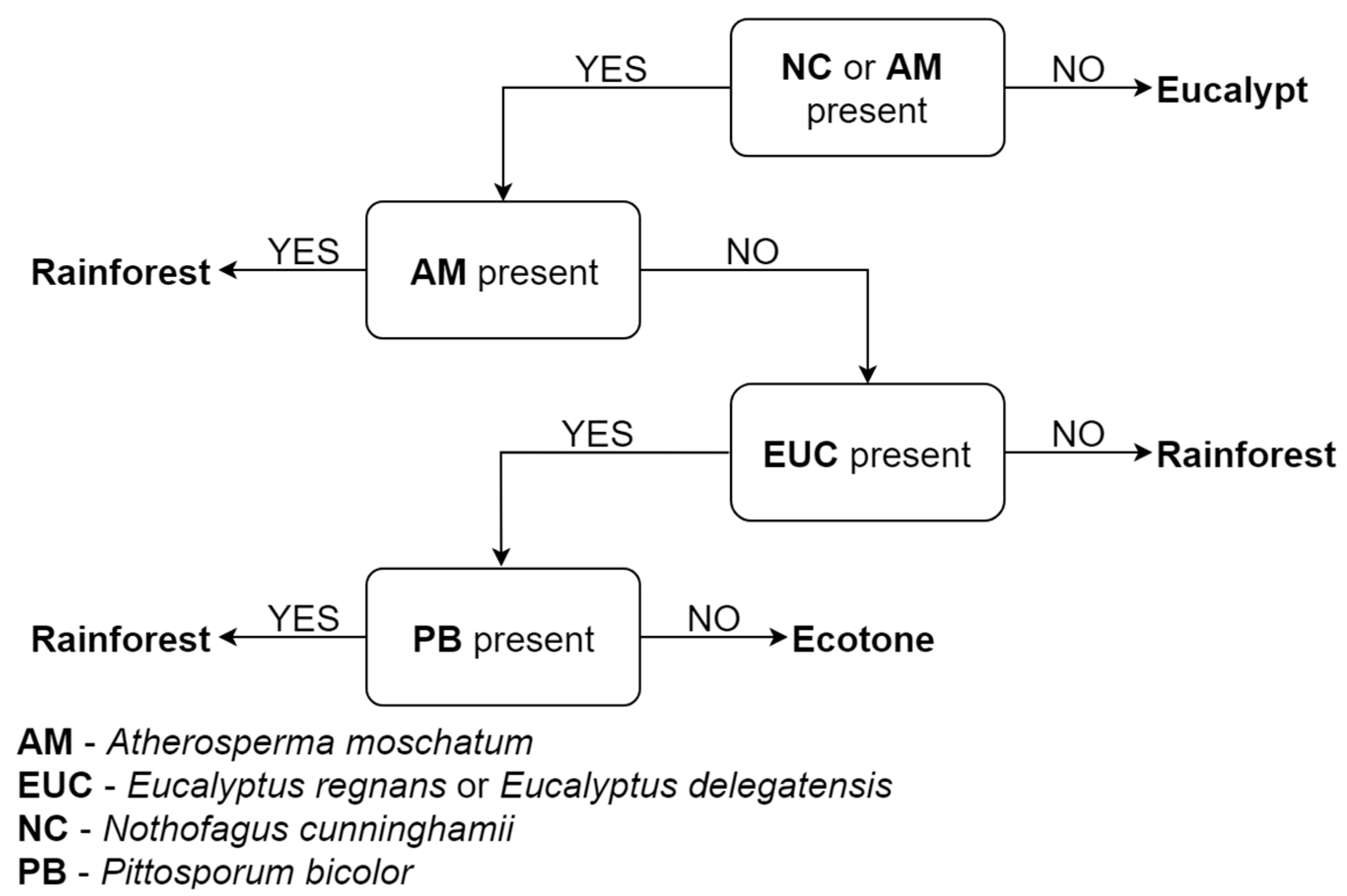
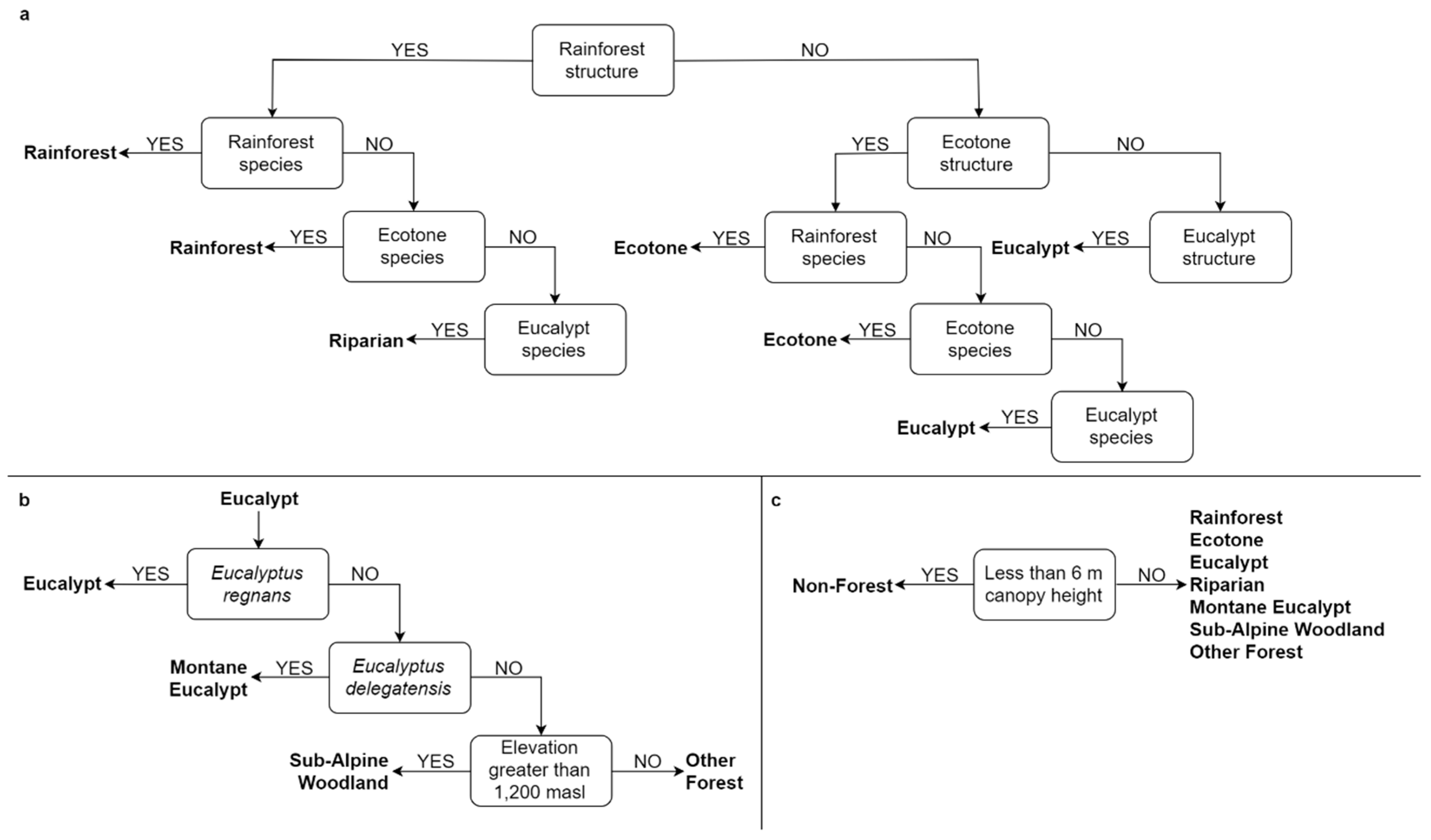
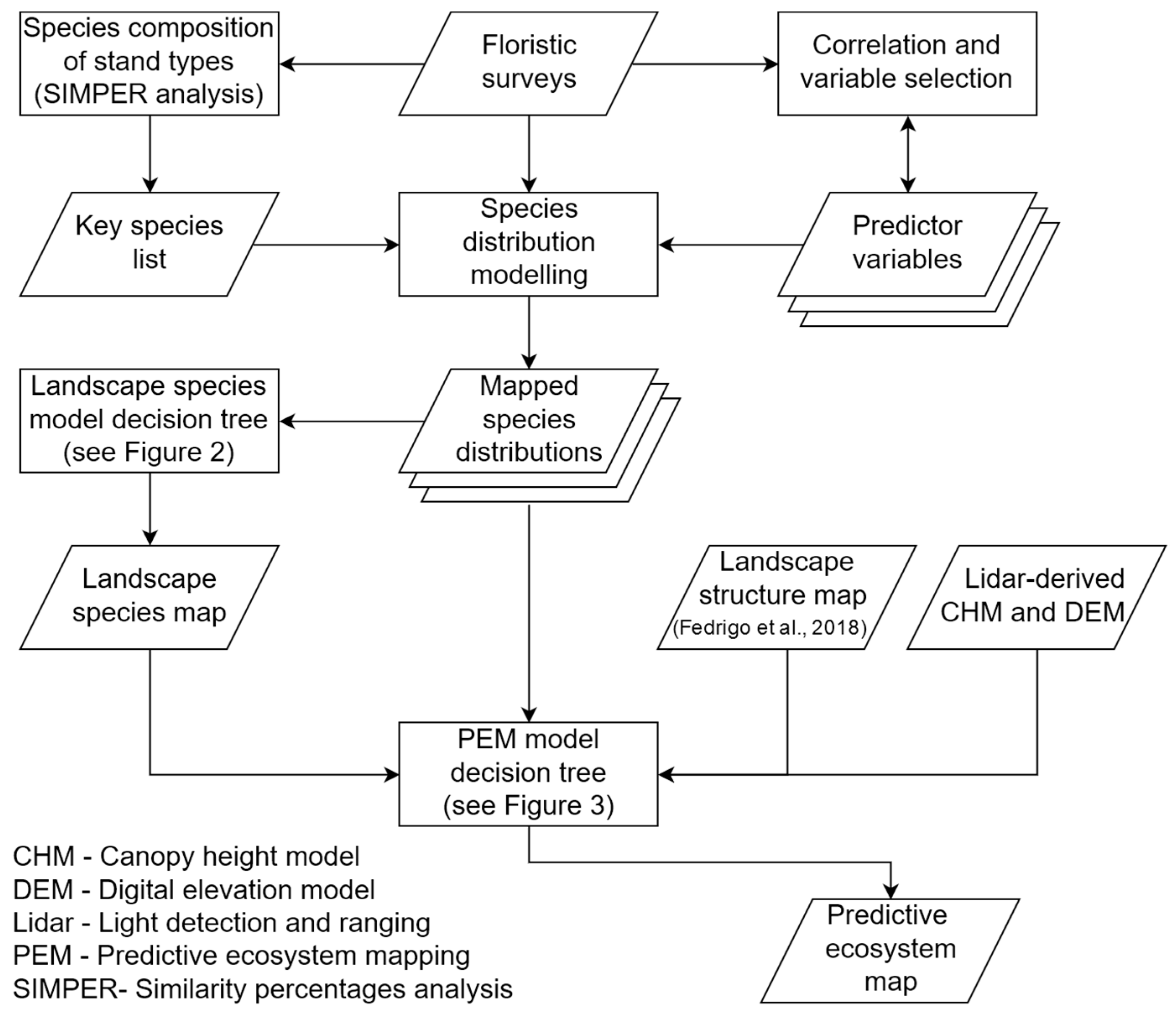
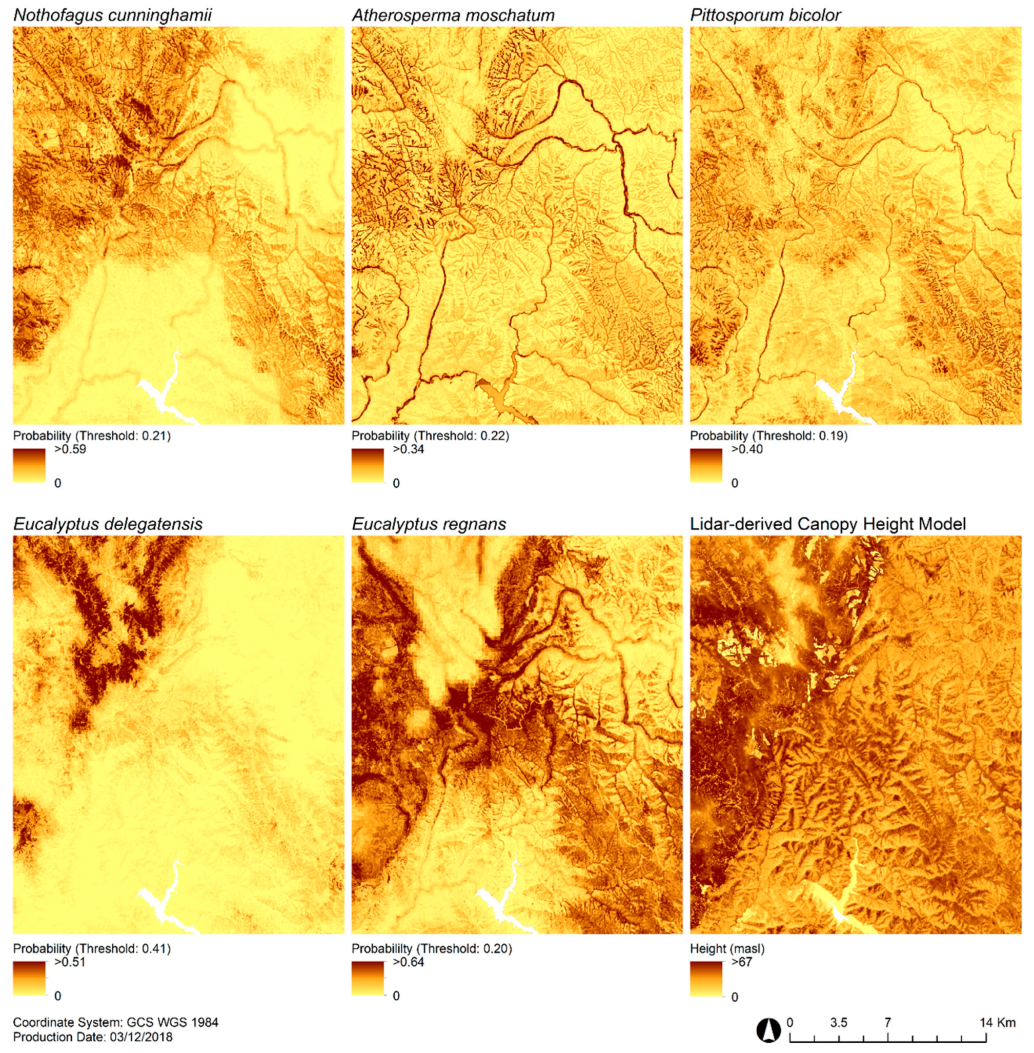
This study seeks to examine the utility of combining recent developments in stand type predictions, using characteristic gradients in lidar structural attributes with complementary sources of ecologically meaningful information. The previously developed lidar-derived stand type map [61] demonstrates the assemble-and-predict approach, which evaluates characteristic gradients (i.e., the vertical profile of vegetation density) across the landscape to predict the distribution of rainforest, ecotone and eucalypt stands. The distribution of species which best characterize stand types in the region were predicted individually and subsequently assembled into community groups in order to provide important ecological context. The lidar-derived and SDM-derived stand type classifications, in addition to auxiliary criteria which further stratify these stand types (i.e., specific individual species, elevation, canopy height) were combined using a series of decision trees to generate a highly detailed PEM model of the study region. This approach to PEM demonstrates a hierarchical, stepwise approach to combining lidar-derived stand type classifications with auxiliary information which provide important ecological context for predicting the spatial distribution of ecological communities. The PEM model demonstrates the potential for defining the spatial distribution of ecological communities at a much higher resolution than existing EVC-based classifications in the study region.

2. Materials and Methods

2.1. Study Area

The Central Highlands region of south-eastern Australia is located in the state of Victoria approximately 100 km north-east of Melbourne (Figure 1). Three spatially contiguous stand types of varying structure dominate the region’s forests: cool temperate rainforest (herein referred to as ‘rainforest’); wet sclerophyll eucalypt forests (‘eucalypt’ forest); and the ‘ecotone’ where rainforest and eucalypt forest species mix [66]. Rainforest stands are dominated by 30–40 m tall Nothofagus cunninghamii, Acacia melanoxylon and Acacia dealbata with understorey species, including up to 20 m tall Atherosperma moschatum. Tree ferns Cyathea australis and Dicksonia antarctica dominate the lower 5 m strata with ground ferns at less than 1 m. Rainforest stands may occasionally include emergent 60 m tall Eucalyptus regnans. Eucalypt stands are dominated by up to 80 m tall E. regnans and occasionally Acacia-dominated understories reaching 40 m in height. Smaller trees and single-stemmed tall shrubs frequently occupy the lower 20 m of these forests. Ecotone forests occur in areas between distinct rainforest and eucalypt stands when eucalypts are co-dominant with rainforest trees in the overstorey above a rainforest understorey. Cameron [62] describes this ‘ecotone stand type’ as ‘cool temperate mixed forest’; a seral community where fire or other recurring disturbances prevent secondary succession to eucalypt-free rainforest.
Other stand types that may be dispersed within or surrounding rainforest, eucalypt and ecotone forests, include a range of eucalypt-dominated forests. Dry sclerophyll forests occur at lower elevations (up to approximately 900 m) and on warm and dry sites (elevated ridge lines and exposed northerly aspects). These dry eucalypt forest canopies are typically dominated by a mix of stringybark, peppermint, and gum-barked eucalypt species, excluding E. regnans and/or E. delegatensis. Similar in dominant overstorey species to wet forest stands, damp eucalypt forest occurs from 200 to 1000 m in elevation on warm, moist sites and contain local abundances of E. obliqua and E. regnans with both species replaced at higher elevations (approximately > 1000 m) by E. delegatensis. Areas of shrubby wet forest are similar to damp eucalypt forest but more consistently dominated by E. delegatensis and a dense understorey of tall shrubs, including Polyscias sambucifolia and Oleria phlogopappa. Montane eucalypt forests include both wet and damp forests, typically at elevations greater than 1000 m, often with a dominance of E. delegatensis that replaces other lower elevation eucalypt species. Sub-alpine woodlands occur at elevations above 1200 m, frequently receive snow, and are dominated by E. pauciflora. Riparian eucalypt forests occur as narrow buffers around inland waterways at lower elevations and occur as patches amongst rainforest at their ecotone. Riparian stands commonly contain E. regnans, E. viminalis, A. melanoxylon and a dense assemblage of understorey vegetation.

2.2. Species Composition of Stand Types

Ecological vegetation classes (EVCs) are used across Victoria to classify vegetation types in different bioregions, defined by climate, geomorphology, geology, soils and vegetation [64,65,67]. EVCs are characterized by floristics, lifeforms and ecological characteristics, with an inferred association to distinct environmental conditions [64,65,67]. Many of these characteristics were either from previously modelled data, derived from Landsat imagery, or from floristic information collected in 2004 and 2005 from an unspecified number of field plots across Victoria [65]. Multiple EVCs correspond to the stand types in this study, including cool temperate rainforest, wet forest, damp forest, shrubby wet forest, riparian forest, montane wet forest, montane damp forest, and sub-alpine woodlands. To facilitate analysis, the wet forest, damp forest, and shrubby wet forest were considered eucalypt stands, and the montane wet and montane damp forest classes were considered as montane eucalypt stands. Cool temperate rainforest, riparian forest, and sub-alpine woodlands retain their classification. There is currently no distinct EVC for ecotone stands. Benchmark lists of species were identified as ‘typical’ to each EVC [68], and were filtered to include only tree, shrub, and tree fern lifeforms.

2.3. Floristic Sampling

Floristic surveys were conducted in 71 field plots (after excluding burnt/logged/observably disturbed plots) that represented our three main stand types (rainforest, ecotone, and eucalypt) from four field campaigns in the study area between April 2011 and October 2014. The presence or absence of all native tree, shrub, and tree fern species were recorded across sites over a broad range of environmental conditions for each stand type (see Section 2.1 Study Area) in fixed-area plots of sizes 20 × 20, 30 × 30, or 10 × 40 m2 (Table S1). Differences in species composition (dependent variable) among stand types (fixed factor) were tested using permutational ANOVA (PERMANOVA), using PERMANOVA+ Version 1.0.6 (PRIMER-E Ltd., Plymouth, UK) [69]. Species composition was based on the Bray-Curtis similarity matrix of the presence or absence of all tree, shrub, and tree fern species. Significance testing of the Bray-Curtis similarity measures and post hoc comparisons were made using 9999 permutations. Permuted residuals were calculated using the Type III (partial) partitioned sum of squares [69]. The similarity percentages (SIMPER) procedure of PRIMER (Version 6.1.15, PRIMER-E Ltd., Plymouth, UK) [70] was used to identify those species that contributed up to 90% similarity within stand types (Table S2) and also those species contributing most to differences among the three main stand types (Table S3). The results of the SIMPER analysis were used to differentiate stand types based on the presence or absence of key species. Species that had an average abundance value of <0.2 (occurs less than 20% of the time) in at least one stand type and also present on the EVC species lists were identified as species which best separate stand types. An exception was made to include E. delegatensis in future analyses as it exists in montane eucalypt forest and typically occurs at elevations between 500 m and 1200 m above sea level [71,72] but was under-represented in the field sampling.

2.4. Lidar-Derived Digital Elevation Model (DEM)

Airborne lidar data were commissioned by the state environment department and were acquired from late 2007 to early 2008 over a subset of the Central Highlands region (Figure 1) from a fixed wing aircraft (Data agreement number DQ201206071138; see Table 1 for flight details and sensor settings). There should be limited impact of the date discrepancy between the lidar capture and floristic sampling due to the slow change in forest structure of these mature stand types (>100 years old) and the exclusion of disturbed field sites in the study [45,51,73,74]. This is further supported by a previous study where a time lag of six years between field-data collection and lidar acquisition only had a minimal influence on the predicted distribution of bird species modelled using structural variables in an undisturbed coniferous forest [74]. All mapping in this study was constrained within the lidar coverage. Data were provided in 2 km × 2 km tiles, including a ‘bare-earth’ digital elevation model (DEM) at 1 m resolution that was generated by the data provider using the ground-classified points. Cells were aggregated and the mean value was used to generate a 20 m resolution DEM for each tile. The reported DEM vertical (±50 cm) and horizontal accuracies (±35 cm) were the same as the lidar data (Table 1). Additional assessments of vertical accuracy were conducted using differential GPS coordinates of six field plots in each of the rainforest, ecotone, and eucalypt stand types of varying vegetation density (total of 18 point locations). Differential GPS (DGPS) coordinates were acquired using a Leica GNSS Viva GS10 with an AS10 antenna and post-processed with ground-based reference stations. The overall root mean square error (RMSE) of the DEM compared to the DGPS recorded elevation at the 25 locations was 0.49 m.

2.5. Environmental and Satellite Data

A series of topographic, climate and satellite-derived characteristic variables were considered for modelling individual species distributions (Table 2). All topographic variables were generated using the 20 m lidar-derived DEM. Seasonal fractional cover products (bare ground, green vegetation, non-green vegetation) derived from Landsat imagery (30 m cell resolution) and acquired between December 2007 and February 2008 [75,76,77] were used as satellite-derived characteristic variables. The combination of the environmental and satellite data at varying resolutions reflects the scale of phenomena at which species distributions are driven or constrained by each variable [3,78]. Each of the satellite-derived characteristic variables and climate variables were resampled to 20 m resolution using bilinear and nearest neighbor interpolation, respectively, for all data analysis and spatial predictions.
Climate variables were developed using a combination of pre-existing and interpolated mean monthly datasets (250 m cell resolution) centered on the 1981–2010 reference period. A series of 19 bioclimatic indices commonly used in SDM analyses were computed using the dismo package [82] in R (Version 3.3.0) [83]. The annual and summer (from December to February) mean vapor pressure deficit (VPD), and an annual heat moisture index (AHMI) were also calculated using the available climate data. Maximum and minimum temperature layers were sourced from a previous study [84], which used a topographic index of relative elevation (minimum temperature only) and standardized moderate resolution imaging spectroradiometer (MODIS) land surface temperature (LST) data to improve interpolation performance. Precipitation and vapor pressure were interpolated using ANUSPLIN 4.4 [85,86] following Stewart et al. [87], with the addition of a regression procedure [84,88] to minimize bias in the monthly climate normals prior to model calibration. Pooled cross-validation statistics for mean monthly precipitation and vapor pressure are presented in Table S4. The mean monthly vapor pressure deficit was then computed by subtracting vapor pressure from the saturation vapor pressure. Saturation vapor pressure (SVP) was calculated using temperature data in conjunction with the August-Roche-Magnus equation [89,90]:
S V P = 6.1094 × e x p   17.625 × T 243.04 + T
where T is the mean monthly temperature.
Correlation matrices were used to detect collinearity and to select a reduced set of predictor variables for SDMs (Table S5). Variables were considered as highly correlated where r ≥ |0.7| [91]. Three climate metrics (annual heat-moisture index [81], temperature seasonality [92], temperature annual range) were selected after excluding highly correlated variables. The majority of climate variables were highly correlated with one another, including the mean annual temperature and the annual precipitation despite smoothing to account for the lack of short-range (5–10 km) correlation between precipitation and elevation [93,94]. As an alternative, the annual heat moisture index was used as it reflects moisture availability as a function of both temperature and precipitation [81]. The three climate variables selected were considered suitable for species distribution modelling, as they reflect both mean climates and seasonal variability, quantifying important components of the ecological niche. Correlation analysis of the optical satellite characteristic gradients showed a strong correlation between the green vegetation and non-green vegetation fractions (r = −0.98). Only the non-green vegetation fraction and bare ground fraction were retained as they were the only pairwise combination below the correlation threshold (r = 0.56). As each of these three cover components (approximately) sum to one, the green vegetation fraction can otherwise be inferred by the bare ground and non-green vegetation cover and therefore was unlikely to have deleterious effects on model performance. The final set of predictor variables included seven environmental variables and two satellite-derived fractional cover products (Table 2).

2.6. Species Distribution Modelling

SDMs for each of the five species which best differentiated stand types were fit using presence and absence records obtained across the Central Highlands region with the randomForest package [95,96] in R. Records were collated from a collaborative network of field plots among the listed authors, (including the 71 sites used for the SIMPER analysis) in addition to project-specific survey data obtained from the Victorian Biodiversity Atlas [97]. Each of the plots used for the analysis maintained a minimum separation distance of at least two pixels (at 20 m resolution), ensuring that no replicates were present in the complete dataset. A six-fold, spatially blocked cross-validation strategy was applied using the blockCV package in R [98] in order to minimize the effect of spatial autocorrelation on the model evaluation. Autocorrelation range in the prediction surfaces was evaluated by fitting variograms to subsampled points across the landscape. A median autocorrelation range of approximately 25 km was selected based on the variogram analysis and was used to stratify the plot data into six sets of training and testing data. Two random forest model variants were run for each species; one using environmental variables only and the other using environmental and satellite variables combined. The cross-validated predictive performance of each model was assessed using the area under the receiver operating characteristic (AUC), overall accuracy (%), sensitivity (%; true positive rate), specificity (%; true negative rate) and true skill statistic (TSS; sensitivity + specificity − 1). The optimal threshold for binary classification (presence or absence) of species distributions was selected by maximizing the sum of sensitivity and specificity of cross-validated predictions [99]. The final set of predictor variables used to map the distribution of each species was selected based on the overall accuracy of the classified cross-validated predictions. The spatial distributions of each species were calculated as the average value predicted by models generated during cross-validation and were classified into binary maps using the optimal threshold.

2.7. Predictive Ecosystem Mapping Model

The PEM model was developed using a combination of SDM-derived (landscape species model) and lidar-derived (landscape structure model) stand type classifications (rainforest, ecotone or eucalypt), individual SDMs, elevation, and a canopy height model (CHM) to identify non-forest areas. The landscape species model was developed using individual species distributions to minimize model complexity while maximizing the number of species presence and absence records used to support stand type classification. Structured survey records could therefore be sourced from ecological surveys with varying objectives and locations, which would not otherwise have been possible with a JSDM approach. We intentionally excluded the full vertical profile of vegetation from the modelling of individual species distributions as they reflect a complex assemblage of multiple species. Each modelled species had between 316 and 494 combined presence and absence records sourced from a selection of different field campaigns conducted in the region. The landscape species model was generated with the predicted distributions of species which best differentiated stand types, guided by a decision tree developed using the SIMPER analysis results (Figure 2). The presence or absence of E. regnans or E. delegatensis was used to differentiate between ecotone and rainforest stands in the landscape species model.
The landscape structure model refers to a specific landscape-scale map derived using structurally based characteristic gradients derived from the full vertical profile of lidar data [61]. The landscape structure model, previously developed by Fedrigo et al. [61] for the same study extent, provides a detailed delineation of forest classes into rainforest, ecotone and eucalypt stands, specifically recognizing the coalescing of stand types at the landscape scale. The model uses known stand types in conjunction with the first 10 principal components of 1 m strata plant area volume density (PAVD) profiles to predict rainforest probability across the landscape. The retained principal components were most sensitive to PAVD for strata between 1 and 10 m. The highest rainforest probabilities were associated with high PAVD in these strata. The classification was then performed by selecting probability thresholds, which were used to separate each stand type [61]. The landscape structure model achieved an overall accuracy of 83.8% and achieved a Cohen’s kappa coefficient of 0.62 during cross-validation, indicating substantial model agreement. Stand type rainforest probability thresholds were adjusted from Fedrigo et al. [61] to ranges that were predicted for field plots only. The rainforest probability range thresholds for eucalypt, ecotone and rainforest stands were <18%, 18% to 70%, and ≥70%, respectively. New thresholds were selected to eliminate potential bias from modelled EVC classifications, which were used to identify thresholds in Fedrigo et al. [61]. The new thresholds resulted in substantial model agreement with the same overall accuracy of 83.8% and a slightly increased Cohen’s kappa coefficient of 0.63. The species distribution modelling and hierarchical decision trees were designed to provide an ecological basis for constraining and further stratifying the lidar-derived stand type maps.
The landscape species model was combined with the landscape structure model to find areas of agreement based on a second decision tree (Figure 3). Congruence between the landscape species and landscape structure models was indicative of a higher degree of confidence in the modelled predictions. E. regnans, E. delegatensis, and elevation were used to separate montane eucalypt, sub-alpine woodland, and other forest types (inclusive of dry forest) from the broader eucalypt class. The CHM was used to filter out non-forest regions and was generated from the lidar data by identifying the maximum height of returns for each cell. Areas of recent logging, within the last 10 years before lidar acquisition, were used to identify a CHM threshold to identify areas of non-forest. A threshold of 6 m was defined as the first quartile CHM value in recently logged areas. All areas on the landscape with a CHM value of less than 6 m were classified broadly as non-forest.
A summary of the preceding steps, and the workflow for developing the final PEM model is illustrated in Figure 4.
The final PEM model was compared against the EVC distributions by summarizing the predicted spatial coverage (km2) of each stand type. The potential distribution of the ecotone stand type amongst the existing EVCs was also examined, as ecotones were not previously defined in the EVCs. The total area of rainforest, ecotone, and eucalypt stands predicted by the landscape species model and the landscape structure model were also compared to highlight how each of these preliminary classifications constrained one another. Total area and percentage of the total ecotone area was determined for each EVC. All comparisons were made separately for two 5 km × 5 km extents (Figure 1) and the full study area.

3. Results

3.1. Species Composition of Stand Types

A total of 19 species occurred in both the collated EVC list and the field-based list of species that were identified as contributing up to 90% of the similarity within each stand type (Table S2). The overall species composition differed significantly among stand types (P ≤ 0.001). Four species, including A. dealbata, A. moschatum, N. cunninghamii, and P. bicolor, were identified as those which were best able to separate stand types based on the SIMPER analysis (Table S3). E. regnans and E. delegatensis were also included to separate ecotone from rainforest stand types in the landscape species model. Rainforest stands were best separated from ecotone and eucalypt stands by the presence of A. moschatum and P. bicolor and the absence of A. dealbata (Table S3). The presence of N. cunninghamii also distinguished rainforest from eucalypt stands. Ecotone stands were best separated from the other stand types by the presence of N. cunninghamii and A. dealbata. While A. dealbata was identified as important in separating rainforest from ecotone and eucalypt stands, it was excluded from the categorization of stand types due to its ecological niche covering the majority of the study area.

3.2. Species Distribution Modelling

Cross-validated error statistics for the five SDMs used to generate the landscape species model and final PEM model are shown in Table 3. Models using environmental and satellite variables achieved a 2% or greater improvement in overall accuracy during cross-validation relative to environmental variables only for E. delegatensis, E. regnans, N. cunninghamii and P. bicolor. Alternative metrics generally supported the selection of the environmental and satellite models based on the trade-off between the true positive and negative rates, and AUC scores (although AUC for P. bicolor was slightly higher for environmental variables). The cross-validation performance was higher across all metrics when using environmental variables for A. moschatum. The annual heat moisture index and fraction of non-green vegetation were consistently among the most important variables across cross-validation folds (see Figure S1 for variable importance plots). The predicted distributions of each species for a subset of the study area are mapped alongside canopy heights in Figure 5.

3.3. Predictive Ecosystem Mapping and Comparison With Ecological Vegetation Classes

The landscape species model and the landscape structure model both predicted much larger areas of rainforest and eucalypt stands in comparison to the PEM model (Table 4). This overestimation was particularly excessive for the landscape species model, where the predicted area was 509.2% more for rainforest, and 234.5% more for eucalypt forest in comparison to the PEM. The landscape structure model also overestimated the total amount of rainforest and eucalypt forest relative to the PEM by 70.6% and 46.4%, respectively. The total ecotone area predicted by the landscape species model was somewhat lower than the PEM (−26.9%), but several times larger for the landscape structure model (347.4%).
These differences are illustrated by the stand type distributions predicted by a spatial subset of the landscape species model and landscape structure model illustrated in Figure 6 alongside corresponding PEM and EVC maps. The distribution of ecotone predicted by the landscape structure model was strongly constrained by the ecologically based landscape species model. Conversely, the structural information provided in the landscape structure model constrained the distribution of rainforest and eucalypt stands which would have otherwise been expected using the landscape species model alone. When combining these classifications, in conjunction with the auxiliary criteria listed in the decision trees (i.e., E. regnans and E. delegatensis distributions, elevation and canopy height), the final PEM model predicted a highly complex distribution of forest across the landscape (see Figure S2 for the full study region). The PEM model indicates a realistic mosaic of stand types with many examples of rainforest transitioning to ecotone, which is interspersed within eucalypt forest.
The EVCs (see Figure S3 for the full study region) predict much larger, more uniform clumps of stand types. The distribution of montane eucalypt and sub-alpine woodland predicted by the PEM model corresponds well to the EVC distributions of equivalent classes. Thick corridors of riparian forest indicated by the EVCs were much thinner, or not present, in the PEM model. Non-forest and regions of other stand types predicted by the PEM model indicate the absence of E. delegatensis and E. regnans, or a canopy height less than 6 m.
Differences in the area covered by each PEM model class and EVCs for the complete study area and both 5 km × 5 km extents were calculated (Table 5). The PEM model predicted 56.2% of the landscape as covered by other forest or non-forest (2909.7 km2), in contrast to the EVCs which predicted 47.0% as covered by all other vegetation classes or non-forest (2429.5 km2). The wet forest, damp forest, and shrubby wet forest EVCs covered a larger area of the landscape (1688.5 km2) than the associated eucalypt class of the PEM model (1169.4 km2). The PEM model had higher area estimates for rainforest (128.6 km2 vs. 101.8 km2) and the only estimate for ecotone (652.9 km2). The EVCs had higher area estimates for riparian forest (204.3 km2 vs. 90.8 km2) and the combined montane wet forest (458.0 km2) and montane damp forest (211.5 km2) when compared against the associated montane eucalypt class of the PEM model (132.9 km2). The PEM model predicted a slightly larger area of sub-alpine woodland than the EVCs (90.6 km2 vs. 81.3 km2). Ecotone stands identified by the PEM model contained multiple EVCs, but were most commonly found in the wet forest, damp forest and montane wet forest EVCs (35.3%, 13.9% and 26.4% of the total ecotone area, respectively; Table 6). The least common EVCs located within the ecotone region were riparian forest, montane damp forest, cool temperate rainforest and sub-alpine woodland (4.8%, 5.2%, 6.5%, and 1.4% of the total ecotone area, respectively).
A visual comparison of the PEM model and the EVC distributions in each 5 km × 5 km extent (see Figure 1 for locations) indicated good general agreement for rainforest and eucalypt forest areas (Figure 7). In general, the finer-scale resolution of the PEM model differentiated stand type patches in contrast to the more continuous distributions of the EVC map. A network of rainforest patches, evident in the bottom left of the first PEM subset, was absent from the EVC map. In contrast, rainforest in the second subset was patchy and covered less area than the cool temperate rainforest EVC.

4. Discussion

The fusion of statistical analyses, lidar-derived structural profiles, and an assemblage of SDMs demonstrates an integrated approach to PEM that was highly sensitive to spatial variations in vegetation structure. The field observations are complemented by the continuous coverage of remote sensing information that indirectly quantifies characteristics of the stand function [
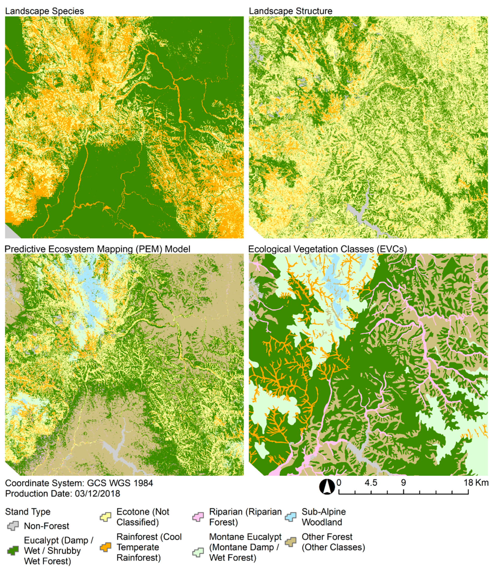
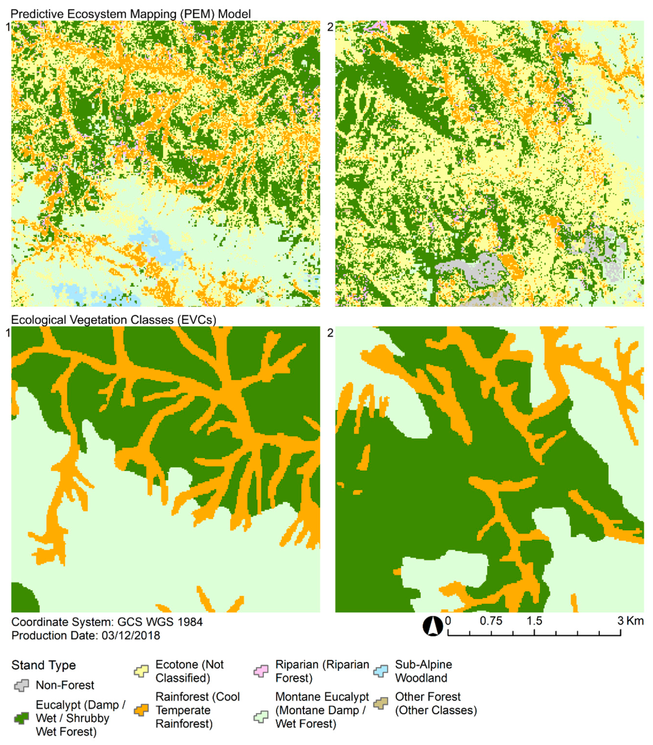
3]. The potential importance of capturing this spatial variability is highlighted when comparing the PEM model against the EVCs that are commonly used in the region. The PEM model shows a much greater level of detail in comparison to the EVCs, which are often spatially homogenized with large clusters of uniform stand types. In the little detailed information that has been published about the development of EVCs, it has been suggested that elements of structure were included in the classification process [65]. Structure (spatial arrangement of forest components) variables in modelling are often used interchangeably with attributes describing function (forest processes) and composition (species abundance and diversity), where details related to one can be used as a proxy for another [41]. The extent, level of detail, and number of variables by which forest structure can be defined by lidar differs greatly in magnitude from the in situ measurements and those derived from optical remote sensing data like Landsat data [54].
The high spatial variability of the PEM model suggests that many stand types do not have as continuous a cover as suggested by the EVC distributions, and this is consistent with our extensive field observations of these landscapes. Despite these differences in spatial resolution, there was generally a good level of agreement in the extent and locations of similar stand types predicted by the PEM model and the EVC maps. Our analysis highlights how complex structural and ecological information can complement one another through different modeling pathways. The lidar-derived landscape structure model was effective at constraining the much broader predictions of rainforest and eucalypt stands by the landscape species model. Conversely, the landscape species model was crucial in providing an ecological basis for constraining predictions of ecotone as indicated by the landscape structure model. Leveraging the congruence between predictions driven by characteristic and environmental gradients shows promise for mapping ecotone stands, as they are likely to have the most dynamic distributions.
Lidar-derived characteristic gradients provide a continuous representation of the full vertical vegetation profile, which is useful for identifying the structural gradient between rainforest, ecotone, and eucalypt stands. Lidar can resolve understorey structure with a level of detail that would not otherwise be possible using characteristic gradients derived from optical remote sensing [3,29,54]. This vertical complexity can be measured at very broad spatial scales using lidar data, and repeat acquisitions can provide valuable opportunities to refine model performance and identify important structural changes in vegetation between specific points in time across the landscape. While field observations were limited to undisturbed stands, the output PEM model may be subject to error in the landscape structure model due to the time difference between field observations and lidar capture. Future studies would benefit from coincident field observation and lidar capture. Furthermore, airborne lidar provides a consistent measurement of structure at a scale that is not possible from the ground, including in regions with limited ground access. Nonetheless, one of the main limitations of using purely structural information to predict stand types is that the tolerance of the individual species that comprise these ecosystems to environmental conditions is not considered [49,61]. For example, eucalypt forest and montane eucalypt forest share similar structural characteristics but are strongly delineated by the environmental conditions that are suitable for either E. regnans or E. delegatensis. By incorporating SDMs into the PEM model, an ecological basis for stand type classification can be determined independently of isolated lidar-derived classifications [96].
Lidar-derived structural profiles were intentionally excluded as predictors for SDMs, as the PAVD profiles represent assemblages of vegetation and their inclusion would have resulted in a large increase in model complexity [49,61]. The use of lidar in SDMs has typically included several lidar-derived metrics [12,56,57,59] rather than some derivative that leverages the entire stream of data collected along the vertical profile. Zimble et al. [12] used airborne lidar-derived tree heights to classify western United States forests into single- and multi-layered stands with > 90% accuracy to be used as the structural component to a variation of the United States Forest Service PEM called habitat decision-support systems. Recent studies that have utilized these profiles have expressed similar challenges in distinguishing stand types with similar vertical vegetations structure [49]. In this study, the use of maximum canopy height as a lidar metric was not useful for distinguishing stand types because E. regnans occurs across most of the landscape and grows to consistent maximum heights.
Recent studies [this study, 29,51,55] have identified how remotely sensed gradients constrain the compositional space of stand or community types based on observed changes in forest structure at different successional stages. Hakkenberg et al. [29] explores the use of an alternative approach to modeling community continua by incorporating lidar and hyperspectral remote sensing. Their study utilizes compositional ordination to summarize plot species information into axes of maximum floristic variation (similar to Simonson et al. [51]). Hakkenberg et al. [29] then classified communities using an unsupervised classification approach utilizing goodness-of-clustering evaluators and dissimilarity matrices. This approach is different to our study but achieves similar outcomes to the SIMPER analyses we used by identifying species that characterize forest communities based on underlying matrices of floristic dissimilarity. The use of dissimilarity matrices (e.g., Ferrier et al. [100]) in both species information [this study, 29] and lidar-only metrics [55] is increasingly being used to classify forest stand types. Compositional modelling in this study, and both the Hakkenberg et al. [29] and Moran et al. [55] studies utilized random forest for classification due to its generalizability and maximization of predictive accuracy with its ability to balance limited training data and high data dimensionality. Key differences in this study include the use of stand type classifications using the vertical continuum of lidar data through dimension-reduced principal components as predictor variables and the removal of highly correlated predictor variables (i.e., the landscape structure model). The ordination approach detailed in Simonson et al. [51] and Hakkenberg et al. [29] are ideally suited for landscapes with limited a priori knowledge about community/stand species composition while the approaches detailed in Moran et al. [55] and Fedrigo et al. [61] are suitable when considering classification using lidar-only metric and vertical continuum data, respectively. This study utilizes a priori knowledge of stand type composition, combined with the SIMPER approach to species classification at the landscape scale prior to the use of lidar data, for further stand type identification. Other studies that have performed similar classifications have been in less complex forests in North America [29] and Europe [51], while our study demonstrates the success of similar PEM approaches in structurally complex (multi-layered, dense, closed canopy temperate) forests of south-eastern Australia. All recent PEM studies highlight concerns with mapping stand or community types as discrete units, when their distribution across the landscape are ultimately continuous and can often overlap in areas of transition [29,55,61].
The PEM model developed as part of this research provides the first spatial prediction of dominant stand types in the study region that considers both the ecological niche and the vertical continuum of vegetation structure. Lidar can penetrate forest canopies and can resolve understorey structure with a level of detail that would not otherwise be possible using characteristic gradients derived from optical remote sensing. Lidar-derived characteristic gradients are therefore particularly useful for identifying ecotone stands that are characterized by eucalypt overstorey with rainforest associated understorey. Cameron [62] defined these ecotone stands as ‘cool temperate mixed forest’ but until now they have not been formally delineated. The ecotone may be the most likely to change in distribution due to the regeneration dynamics that occur in these stands with changes in microclimate, disturbance regimes and light conditions [62,63]. The succession of forest stands from one type to another suggests that these stand type maps reflect dynamic processes and will require regular assessment to evaluate their agreement with ground observations [50,58]. Repeat lidar acquisitions over time will provide opportunities to detect changes in the structure and distribution of these stand types in response to natural and anthropogenic disturbances at very high spatial resolutions.

5. Conclusions

This study demonstrates a novel approach to PEM that integrates a range of data types including field-based, optical remotely-sensed, and lidar data to model the continuous distribution of key stand types in the temperate forests of south-eastern Australia. By exploring the use of varying environmental and characteristic predictor variables and identifying those species which best separated stand types, we generated a landscape species model based on the combination of multiple SDMs. Characterizations of stand types based on significantly different species compositions and lidar structural profiles were critical to identifying and mapping the predicted distribution of ecotone between rainforest and eucalypt stands. Using a combination of SDMs and remote sensing data, the ecotone forest was clearly mapped for the first time, offering potential for finer-scale mapping of forests in landscapes beyond the temperate forests of south-eastern Australia. The PEM model allows processes influencing forest development patterns to be captured which should enhance classification accuracy and provide a baseline for evaluating changes in forest development over time. More detailed and high-resolution stand type mapping for this region and others will serve to improve our knowledge of the composition and structure of forested landscapes, and provide a valuable tool for supporting sustainable forest management decisions.

Supplementary Materials

The following are available online at https://www.mdpi.com/2072-4292/11/1/93/s1, Table S1: Floristic survey and sampling strategies for the four (1–4) sampling campaigns used in this study, Table S2: SIMPER analysis on presence and absence records of tree, shrub, and tree fern species across 71 field plots in rainforest, ecotone and eucalypt stands (average similarity within stand types in brackets). Bold species occur in both the field floristics and ecological vegetation class species list for similar stand types, Table S3: SIMPER analysis among rainforest, ecotone, and eucalypt stands based on presence and absence records of tree, shrub, and tree fern species across 71 field plots. Bold species were used to separate stand types based on an abundance value < 0.2 in at least one stand type, Table S4: Spatially and temporally pooled cross-validated error statistics for mean monthly (1981–2010) precipitation and vapor pressure across Victoria interpolated using ordinary trivariate splines, Table S5: Correlation matrix of variables considered for species distribution modelling across the study region, Figure S1: Random forest variable importance plots for distribution models of species which characterize rainforest, ecotone and eucalypt stand types. Figure S2: Map of stand type distributions as predicted by the predictive ecosystem mapping model within the lidar footprint acquired across the Central Highlands region. Figure S3: Map of stand type distributions as predicted by the ecological vegetation classes within the lidar footprint acquired across the Central Highlands region.

Author Contributions

M.F. and S.B.S. developed methodology, performed formal analysis, validation, visualization, interpreted results and wrote the paper; M.F., S.B.S. and H.V. aided in data curation; M.F., S.H.R., S.K., L.T.B. and C.R.N. contributed to conceptualization, data acquisition, model design and analysis, and paper revisions.

Funding

This research was funded by the Commonwealth Scientific and Industrial Research Organisation (CSIRO) Land and Water Business Unit (formally Sustainable Agriculture Flagship) as well as the Victorian Department of Environment, Land, Water and Planning (DELWP) iFER (Integrated Forest Ecosystem Research) program. Research was undertaken with approval by the Victorian DELWP under research permit numbers 10006440, 10006691, and 10007105.

Acknowledgments

The authors thank James Cook University, Commonwealth Scientific and Industrial Research Organisation (CSIRO), and the Queensland Department of Environment and Science (DES) Remote Sensing Centre for time allowed to complete this manuscript. We would like to thank those who contributed to data collection and processing, including D. Lockwood, B. Smith, J. Najera, L. Parker, B. Minnis, G. Sanders, T. Fairman, M. Chick, and D. Navarrete. We thank all reviewers for their comments towards improving this manuscript.

Conflicts of Interest

The authors declare no conflict of interest. The funders had no role in the design of the study; in the collection, analyses, or interpretation of data; in the writing of the manuscript, or in the decision to publish the results.

References

  1. Franklin, J. Predictive vegetation mapping: Geographic modeling of biospatial patterns in relation to environmental gradients. Prog. Phys. Geog. 1995, 19, 474–499. [Google Scholar] [CrossRef]
  2. Miller, J. Species distribution modeling. Geogr. Compass 2010, 4, 490–509. [Google Scholar] [CrossRef]
  3. Cord, A.F.; Meentemeyer, R.K.; Leitão, P.J.; Václavík, T. Modelling species distributions with remote sensing data: Bridging disciplinary perspectives. J. Biogeogr. 2013, 40, 2226–2227. [Google Scholar] [CrossRef]
  4. Jones, K.; Meidinger, D.; Clark, D.; Schultz, F. Towards the Establishment of Predictive Ecosystem Mapping Standards: A White Paper; 1st Approximation. Prepared for Terrestrial Ecosystem Mapping Alternatives Task Force; Resource Inventory Committee (RIC), Victoria, BC, Canada, 8–9 September 1999; pp. 1–88. [Google Scholar]
  5. Meidinger, D.; Enns, B.; Banner, A.; Jones, C. EcoGen: A model for predictive ecosystem mapping. In Proceedings from Science to Management and Back: A Science Forum for Southern Interior Ecosystems of British Columbia; Hollstedt, C., Sutherland, K., Innes, T., Eds.; Southern Interior Forest Extension and Research Partnership: Kamloops, BC, Canada, 2000; pp. 45–47. [Google Scholar]
  6. Ohmann, J.L.; Gregory, M.J. Predictive mapping of forest composition and structure with direct gradient analysis and nearest-neighbor imputation in coastal Oregon, U.S.A. Can. J. For. Res. 2002, 32, 725–741. [Google Scholar] [CrossRef]
  7. Fraser, R.; McLennan, D.; Ponomarenko, S.; Olthof, I. Image-based predictive ecosystem mapping in Canadian arctic parks. Int. J. Appl. Earth Obs. 2012, 14, 129–138. [Google Scholar] [CrossRef]
  8. Elith, J.; Leathwick, J.R. Species distribution models: Ecological explanation and prediction across space and time. Annu. Rev. Ecol. Evol. Syst. 2009, 40, 677–697. [Google Scholar] [CrossRef]
  9. Kearney, M.; Porter, W. Mechanistic niche modelling: Combining physiological and spatial data to predict species’ ranges. Ecol. Lett. 2009, 12, 334–350. [Google Scholar] [CrossRef]
  10. Nix, H.A.; Busby, J. BIOCLIM, a Bioclimatic Analysis and Prediction System. Annual Report CSIRO; CSIRO Division of Water and Land Resources: Canberra, Australia, 1986.
  11. Pearson, R.G.; Dawson, T.P. Predicting the impacts of climate change on the distribution of species: Are bioclimate envelope models useful? Glob. Ecol. Biogeogr. 2003, 12, 361–371. [Google Scholar] [CrossRef]
  12. Zimble, D.A.; Evans, D.L.; Carlson, G.C.; Parker, R.C.; Grado, S.C.; Gerard, P.D. Characterizing vertical forest structure using small-footprint airborne LiDAR. Remote Sens. Environ. 2003, 87, 171–182. [Google Scholar] [CrossRef] [Green Version]
  13. Hirzel, A.H.; Hausser, J.; Chessel, D.; Perrin, N. Ecological-niche factor analysis: How to compute habitat-suitability maps without absence data? Ecology 2002, 83, 2027–2036. [Google Scholar] [CrossRef]
  14. Vierling, K.T.; Vierling, L.A.; Gould, W.A.; Martinuzzi, S.; Clawges, R.M. Lidar: Shedding new light on habitat characterization and modeling. Front. Ecol. Environ. 2008, 6, 90–98. [Google Scholar] [CrossRef]
  15. Peterson, A.T. Uses and requirements of ecological niche models and related distributional models. Biodivers. Inform. 2006, 3, 59–72. [Google Scholar] [CrossRef]
  16. Stockwell, D.R.B. Improving ecological niche models by data mining large environmental datasets for surrogate models. Ecol. Model. 2006, 192, 188–196. [Google Scholar] [CrossRef] [Green Version]
  17. Booth, T.H. A new method for assisting species selection. Commonw. For. Rev. 1985, 64, 241–250. [Google Scholar]
  18. Austin, M.P. Spatial prediction of species distribution: An interface between ecological theory and statistical modelling. Ecol. Model. 2002, 157, 101–118. [Google Scholar] [CrossRef]
  19. Ferrier, S.; Drielsma, M.; Manion, G.; Watson, G. Extended statistical approaches to modelling spatial pattern in biodiversity in north-east New South Wales. II. Community-level modelling. Biodivers. Conserv. 2002, 11, 2309–2338. [Google Scholar] [CrossRef]
  20. Overton, J.M.; Stephens, R.T.T.; Leathwick, J.R.; Lehmann, A. Information pyramids for informed biodiversity conservation. Biodivers. Conserv. 2002, 11, 2093–2116. [Google Scholar] [CrossRef]
  21. Ferrier, S.; Guisan, A. Spatial modelling of biodiversity at the community level. J. Appl. Ecol. 2006, 43, 393–404. [Google Scholar] [CrossRef] [Green Version]
  22. Guillera-Arroita, G.; Lahoz-Monfort, J.J.; Elith, J.; Gordon, A.; Kujala, H.; Lentini, P.E.; McCarthy, M.A.; Tingley, R.; Wintle, B.A. Is my species distribution model fit for purpose? Matching data and models to applications. Glob. Ecol. Biogeogr. 2015, 24, 276–292. [Google Scholar] [CrossRef] [Green Version]
  23. Maguire, K.C.; Nieto-Lugilde, D.; Fitzpatrick, M.C.; Williams, J.W.; Blois, J.L. Modeling species and community responses to past, present, and future episodes of climatic and ecological change. Annu. Rev. Ecol. Evol. Syst. 2015, 46, 343–368. [Google Scholar] [CrossRef]
  24. Ohmann, J.L.; Gregory, M.J.; Henderson, E.B.; Roberts, H.M. Mapping gradients of community composition with nearest-neighbour imputation: Extending plot data for landscape analysis. J. Veg. Sci. 2011, 22, 660–676. [Google Scholar] [CrossRef]
  25. Clark, J.S.; Gelfand, A.E.; Woodall, C.W.; Zhu, K. More than the sum of the parts: Forest climate response from joint species distribution models. Ecol. Appl. 2014, 24, 990–999. [Google Scholar] [CrossRef] [PubMed]
  26. Pollock, L.J.; Tingley, R.; Morris, W.K.; Golding, N.; O’Hara, R.B.; Parris, K.M.; Vesk, P.A.; McCarthy, M.A. Understanding co-occurrence by modelling species simultaneously with a Joint Species Distribution Model (JSDM). Methods Ecol. Evol. 2014, 5, 397–406. [Google Scholar] [CrossRef] [Green Version]
  27. Cutler, D.R.; Edwards, T.C.; Beard, K.H.; Cutler, A.; Hess, K.T.; Gibson, J.; Lawler, J.J. Random forests for classification in ecology. Ecology 2007, 88, 2783–2792. [Google Scholar] [CrossRef] [PubMed]
  28. Olden, J.D.; Lawler, J.J.; Poff, N.L. Machine learning methods without tears: A primer for ecologists. Q. Rev. Biol. 2008, 83, 171–193. [Google Scholar] [CrossRef] [PubMed]
  29. Hakkenberg, C.R.; Peet, R.K.; Urban, D.L.; Song, C. Modeling plant composition as community continua in a forest landscape with LiDAR and hyperspectral remote sensing. Ecol. Appl. 2018, 28, 177–190. [Google Scholar] [CrossRef] [PubMed]
  30. Recknagel, F. Ecological Informatics: Scope, Techniques and Applications, 2nd ed.; Springer: New York, NY, USA, 2006; pp. 1–496. ISBN 9783540283836. [Google Scholar]
  31. Elith, J.; Graham, C.H.; Anderson, R.P.; Dudík, M.; Ferrier, S.; Guisan, A.; Hijmans, R.J.; Huettmann, F.; Leathwick, J.R.; Lehmann, A.; et al. Novel methods improve prediction of species’ distributions from occurrence data. Ecography 2006, 29, 129–151. [Google Scholar] [CrossRef] [Green Version]
  32. De’ath, G. Boosted trees for ecological modeling and prediction. Ecology 2007, 88, 243–251. [Google Scholar] [CrossRef]
  33. Wilson, B.T.; Lister, A.J.; Riemann, R.I. A nearest-neighbor imputation approach to mapping tree species over large areas using forest inventory plots and moderate resolution raster data. For. Ecol. Manag. 2012, 271, 182–198. [Google Scholar] [CrossRef]
  34. Helmer, E.; Ruzycki, T.; Wilson, B.; Sherrill, K.; Lefsky, M.; Marcano-Vega, H.; Brandeis, T.; Erickson, H.; Ruefenacht, B. Tropical deforestation and recolonization by exotic and native trees: Spatial patterns of tropical forest biomass, functional groups, and species counts and links to stand age, geoclimate, and sustainability goals. Remote Sens. 2018, 10, 1724. [Google Scholar] [CrossRef]
  35. Breiman, L. Random forests. Mach. Learn. 2001, 45, 5–32. [Google Scholar] [CrossRef]
  36. Guisan, A.; Zimmermann, N.E. Predictive habitat distribution models in ecology. Ecol. Model. 2000, 135, 147–186. [Google Scholar] [CrossRef]
  37. Araújo, M.B.; Guisan, A. Five (or so) challenges for species distribution modelling. J. Biogeogr. 2006, 33, 1677–1688. [Google Scholar] [CrossRef]
  38. Heikkinen, R.K.; Luoto, M.; Araújo, M.B.; Virkkala, R.; Thuiller, W.; Sykes, M.T. Methods and uncertainties in bioclimatic envelope modelling under climate change. Prog. Phys. Geogr. 2006, 30, 751–777. [Google Scholar] [CrossRef] [Green Version]
  39. Austin, M.P.; Van Neil, K.P. Improving species distribution models for climate change studies: Variable selection and scale. J. Biogeogr. 2011, 38, 1–8. [Google Scholar] [CrossRef]
  40. Morrissey, R.C.; Jacobs, D.F.; Seifert, J.R.; Kershaw, J.A. Overstory species composition of naturally regenerated clearcuts in an ecological classification framework. Plant Ecol. 2010, 208, 21–34. [Google Scholar] [CrossRef]
  41. McElhinny, C.; Gibbons, P.; Brack, C.; Bauhus, J. Forest and woodland stand structural complexity: Its definition and measurement. For. Ecol. Manag. 2005, 218, 1–24. [Google Scholar] [CrossRef]
  42. Wilkes, P.; Jones, S.D.; Suarez, L.; Heywood, A.; Mellor, A.; Woodgate, W.; Soto-Berelov, M.; Skidmore, A. Using discrete-return ALS to quantify number of canopy strata across diverse forest types. Methods Ecol. Evol. 2016, 7, 700–712. [Google Scholar] [CrossRef]
  43. Wulder, M.A.; White, J.C.; Nelson, R.F.; Næsset, E.; Ole, H.; Coops, N.C.; Hilker, T.; Bater, C.W.; Gobakken, T. Lidar sampling for large-area forest characterization: A review. Remote Sens. Environ. 2012, 121, 196–209. [Google Scholar] [CrossRef] [Green Version]
  44. Lefsky, M.A.; Cohen, W.B.; Parker, G.G.; Harding, D.J. Lidar remote sensing for ecosystem studies. BioScience 2002, 52, 19–30. [Google Scholar] [CrossRef]
  45. Brubaker, K.M.; Johnson, Q.K.; Kaye, M.W. Spatial patterns of tree and shrub biomass in a deciduous forest using leaf-off and leaf-on lidar. Can. J. For. Res. 2018, 48, 1020–1033. [Google Scholar] [CrossRef]
  46. Hopkinson, C.; Chasmer, L.; Young-Pow, C.; Treitz, P. Assessing forest metrics with a ground-based scanning lidar. Can. J. For. Res. 2004, 34, 573–583. [Google Scholar] [CrossRef]
  47. Bergen, K.M.; Goetz, S.J.; Dubayah, R.O.; Henebry, G.M.; Hunsaker, C.T.; Imhoff, M.L.; Nelson, R.F.; Parker, G.G.; Radeloff, V.C. Remote sensing of vegetation 3-D structure for biodiversity and habitat: Review and implications for lidar and radar spaceborne missions. J. Geophys. Res. Biogeogr. 2009, 114, 1–13. [Google Scholar] [CrossRef]
  48. Pirotti, F. Analysis of full-waveform LiDAR data for forestry applications: A review of investigations and methods. iForest-Biogeosci. For. 2011, 4, 100–106. [Google Scholar] [CrossRef]
  49. Marselis, S.M.; Tang, H.; Armston, J.D.; Calders, K.; Labrière, N.; Dubayah, R. Distinguishing vegetation types with airborne waveform lidar data in tropical forest-savanna mosaic: A case study in Lopé National Park, Gabon. Remote Sens. Environ. 2018, 216, 626–634. [Google Scholar] [CrossRef]
  50. Kane, V.R.; McGaughey, R.J.; Bakker, J.D.; Gersonde, R.F.; Lutz, J.A.; Franklin, J.F. Comparisons between field-and LiDAR-based measures of stand structural complexity. Can. J. For. Res. 2010, 40, 761–773. [Google Scholar] [CrossRef]
  51. Simonson, W.D.; Allen, H.D.; Coomes, D.A. Use of an airborne lidar system to model plant species composition and diversity of Mediterranean oak forests. Conserv. Biol. 2012, 26, 840–850. [Google Scholar] [CrossRef]
  52. Broadbent, E.N.; Asner, G.P.; Peña-Claros, M.; Palace, M.; Soriano, M. Spatial partitioning of biomass and diversity in a lowland Bolivian forest: Linking field and remote sensing measurements. For. Ecol. Manag. 2008, 255, 2602–2616. [Google Scholar] [CrossRef]
  53. Liu, X. Airborne LiDAR for DEM generation: Some critical issues. Prog. Phys. Geogr. 2008, 32, 31–49. [Google Scholar] [CrossRef]
  54. Campbell, M.J.; Dennison, P.E.; Hudak, A.T.; Parham, L.M.; Butler, B.W. Quantifying understory vegetation density using small-footprint airborne lidar. Remote Sen. Environ. 2018, 215, 330–342. [Google Scholar] [CrossRef]
  55. Moran, C.J.; Rowell, E.M.; Seielstad, C.A. A data-driven framework to identify and compare forest structure classes using LiDAR. Remote Sens. Environ. 2018, 211, 154–166. [Google Scholar] [CrossRef]
  56. Dubayah, R.O.; Drake, J.B. Lidar remote sensing for forestry. J. For. 2000, 98, 44–46. [Google Scholar] [CrossRef]
  57. Lim, K.; Treitz, P.; Wulder, M.; St-Onge, B.; Flood, M. LiDAR remote sensing of forest structure. Prog. Phys. Geogr. Earth Environ. 2003, 27, 88–106. [Google Scholar] [CrossRef]
  58. Falkowski, M.J.; Evans, J.S.; Martinuzzi, S.; Gessler, P.E.; Hudak, A.T. Characterizing forest succession with lidar data: An evaluation for the inland northwest, USA. Remote Sens. Environ. 2009, 113, 946–956. [Google Scholar] [CrossRef]
  59. Van Leeuwen, M.; Nieuwenhuis, M. Retrieval of forest structural parameters using LiDAR remote sensing. Eur. J. For. Res. 2010, 129, 749–770. [Google Scholar] [CrossRef]
  60. Hakkenberg, C.R.; Zhu, K.; Peet, R.K.; Song, C. Mapping multi-scale vascular plant richness in a forest landscape with integrated LiDAR and hyperspectral remote-sensing. Ecology 2018, 99, 474–487. [Google Scholar] [CrossRef]
  61. Fedrigo, M.; Newnham, G.J.; Coops, N.C.; Culvenor, D.S.; Bolton, D.K.; Nitschke, C.R. Predicting temperate forest stand types using only structural profiles from discrete return airborne lidar. ISPRS J. Photogramm. 2018, 136, 106–119. [Google Scholar] [CrossRef]
  62. Cameron, D. A Field Guide to Rainforest Identification in Victoria: Differential Species Keys for the Delineation of Rainforest Boundaries; Department of Sustainability and Environment: Melbourne, Australia, 2011; ISBN 9781742871219.
  63. Kasel, S.; Bennett, L.T.; Aponte, C.; Fedrigo, M.; Nitschke, C.R. Environmental heterogeneity promotes floristic turnover in temperate forests of south-eastern Australia more than dispersal limitation and disturbance. Landsc. Ecol. 2017, 32, 1613–1629. [Google Scholar] [CrossRef]
  64. Muir, A.M.; Edwards, S.A.; Dickins, M.J. Description and Conservation Status of the Vegetation of the Box-Ironbark Ecosystem in Victoria; Department of Conservation and Natural Resources: Victoria, Australia, 1995.
  65. Department of Sustainability and Environment (DSE), Victorian Government Department of Sustainability and Environment Melbourne. Native Vegetation Information: Native Vegetation Extent Dataset Information Sheet No 3. 2007. Available online: http://www.depi.vic.gov.au/__data/assets/pdf_file/0008/97325/NV_extent_dataset.pdf (accessed on 17 July 2015).
  66. Fedrigo, M.; Kasel, S.; Bennett, L.T.; Roxburgh, S.H.; Nitschke, C.R. Carbon stocks in temperate forests of south-eastern Australia reflect large tree distribution and edaphic conditions. For. Ecol. Manag. 2014, 334, 129–143. [Google Scholar] [CrossRef]
  67. Woodgate, P.W.; Peel, B.D.; Coram, J.E.; Farrell, S.J.; Ritman, K.T.; Lewis, A. Old-growth forest studies in Victoria, Australia concepts and principles. For. Ecol. Manag. 1996, 85, 79–94. [Google Scholar] [CrossRef]
  68. Department of Environment, Land, Water and Planning (DELWP), Victoria State Government. EVC Benchmarks. 2015. Available online: http://www.depi.vic.gov.au/environment-and-wildlife/biodiversity/evc-benchmarks#bioregionname (accessed on 17 July 2015).
  69. Anderson, M.J.; Gorley, R.N.; Clarke, K.R. PERMANOVA+ for PRIMER: Guide to Software and Statistical Method; PRIMER-E Ltd.: Plymouth Marine Laboratory, UK, 2008. [Google Scholar]
  70. Clarke, K.R.; Warwick, R.M. Change in Marine Communities: An Approach to Statistical Analysis and Interpretation; PRIMER-E Ltd.: Plymouth Marine Laboratory, UK, 2001; ISBN 9781855311404. [Google Scholar]
  71. Boland, D.J.; Brooker, M.I.H.; Turnbull, J.W. Eucalyptus Seed; CSIRO: Canberra, Australia, 1980; pp. 1–191.
  72. Close, D.C.; Wilson, S.J. Provenance effects on pre-germination treatments for Eucalyptus regnans and E. delegatensis seed. For. Ecol. Manag. 2002, 170, 299–305. [Google Scholar] [CrossRef]
  73. Fedrigo, M.; Stewart, S.B.; Kasel, S.; Levchenko, V.; Trouvé, R.; Nitschke, C.R. Radiocarbon dating informs tree fern population dynamics and disturbance history of temperate forests in southeast Australia. Radiocarbon 2018, in press. [Google Scholar] [CrossRef]
  74. Vierling, K.T.; Swift, C.E.; Hudak, A.T.; Vogeler, J.C.; Vierling, L.A. How much does the time lag between wildlife field-data collection and LiDAR-data acquisition matter for studies of animal distributions? A case study using bird communities. Remote Sens. Lett. 2014, 5, 185–193. [Google Scholar] [CrossRef]
  75. Scarth, P.; Röder, A.; Schmidt, M. Tracking Grazing Pressure and Climate Interaction—The Role of Landsat Fractional Cover in Time Series Analysis. In Proceedings of the 15th Australasian Remote Sensing and Photogrammetry Conference (ARSPC), Alice Springs, Australia, 13–17 September 2010. [Google Scholar]
  76. Flood, N. Seasonal composite landsat TM/ETM+ images using the Medoid (a multi-dimensional median). Remote Sens. 2013, 5, 6481–6500. [Google Scholar] [CrossRef]
  77. Seasonal Fractional Cover—Landsat, JRSRP Algorithm, Australia Coverage. Joint Remote Sensing Research Program (JRSRP). 2016. Available online: http://auscover.org.au/purl/landsat-seasonal-fractional-cover (accessed on 20 December 2016).
  78. Pettorelli, N.; Wegmann, M.; Skidmore, A.; Mücher, S.; Dawson, T.P.; Fernandez, M.; Lucas, R.; Schaepman, M.E.; Wang, T.; O’Connor, B.; et al. Framing the concept of satellite remote sensing essential biodiversity variables: Challenges and future directions. Remote Sens. Ecol. Conserv. 2016, 2, 122–131. [Google Scholar] [CrossRef]
  79. Conrad, O.; Bechel, B.; Bock, M.; Dietrich, H.; Fischer, E.; Gerlitz, L.; Wehberg, J.; Wichmann, V.; Böhner, J. System for automated geoscientific analyses (SAGA) v. 2.1.4. Geosci. Model Dev. 2015, 8, 1991–2007. [Google Scholar] [CrossRef]
  80. McCune, B.; Mefford, M.J. HyperNiche. Nonparametric Multiplicative Habitat Modeling, version 2; MjM Software: Gleneden Beach, OR, USA, 2009. [Google Scholar]
  81. Wang, T.; Hamann, A.; Spittlehouse, D.L.; Aitken, S.N. Development of scale-free climate data for western Canada for use in resource management. Int. J. Climatol. 2006, 26, 383–397. [Google Scholar] [CrossRef]
  82. Hijmans, R.J.; Phillips, S.; Leathwick, J.; Elith, J. dismo: Species distribution modeling. R package version 1.1-4. 2017. Available online: https://CRAN.R-project.org/package=dismo (accessed on 12 January 2017).
  83. R: A Language and Environment for Statistical Computing; R Core Team, R Foundation for Statistical Computing: Vienna, Austria, 2016. Available online: https://www.R-project.org/ (accessed on 1 January 2013).
  84. Stewart, S.B.; Nitschke, C.R. Improving temperature interpolation using MODIS LST and local topography: A comparison of methods in south east Australia. Int. J. Climatol. 2017, 37, 3098–3110. [Google Scholar] [CrossRef]
  85. Hutchinson, M.F.; Xu, T. ANUSPLIN Version 4.4 User Guide; Fenner School of Environment and Society, Australian National University: Canberra, Australia, 2013. [Google Scholar]
  86. Fenner School of Environment and Society and Geoscience Australia. GEODATA 9 Second Digital Elevation Model (DEM-9S), Version 3; Fenner School of Environment and Society and Geoscience Australia: Canberra, Australia, 2008. [Google Scholar]
  87. Stewart, S.B.; Choden, K.; Fedrigo, M.; Roxburgh, S.H.; Keenan, R.; Nitschke, C.R. The role of topography and the north Indian monsoon on mean monthly climate interpolation within the Himalayan Kingdom of Bhutan. Int. J. Climatol. 2017, 37 (Suppl. 1), 897–909. [Google Scholar] [CrossRef]
  88. Hopkinson, R.F.; Hutchinson, M.F.; McKenney, D.W.; Milewska, E.J.; Padadopol, P. Optimizing input data for gridding climate normals for Canada. J. Appl. Meteorol. Clim. 2012, 51, 1508–1518. [Google Scholar] [CrossRef]
  89. Alduchov, O.A.; Eskridge, R.E. Improved Magnus form approximation of saturation vapour pressure. J. Appl. Meteorol. 1996, 34, 601–609. [Google Scholar] [CrossRef]
  90. Lawrence, M. The relationship between relative humidity and the dewpoint temperature in moist air: A simple conversion and applications. Bull. Am. Meteorol. Soc. 2005, 86, 225–233. [Google Scholar] [CrossRef]
  91. Dormann, C.F.; Elith, J.; Bacher, S.; Buchmann, C.; Carl, G.; Carré, G.; García Marquéz, J.R.; Gruber, B.; Lafourcade, B.; Leitão, P.J.; et al. Collinearity: A review of methods to deal with it and a simulation study evaluating their performance. Ecography 2013, 36, 27–46. [Google Scholar] [CrossRef]
  92. O’Donnell, M.S.; Ignizio, D.A. Bioclimatic predictors for supporting ecological applications in the conterminous United States. US Geol. Surv. Data Ser. 2012, 691, 1–10. [Google Scholar]
  93. Hutchinson, M.F. Interpolation of rainfall data with thin plate smoothing splines—Part II: Analysis of topographic dependence. GIDA 1998, 2, 152–167. [Google Scholar]
  94. Sharples, J.J.; Hutchinson, M.F.; Jellett, D.R. On the horizontal scale of elevation dependence of Australian monthly precipitation. J. Appl. Meteorol. 2005, 44, 1850–1865. [Google Scholar] [CrossRef]
  95. Liaw, A.; Wiener, M. Classification and regression by randomForest. R News 2002, 2, 18–22. [Google Scholar]
  96. Prasad, A.M.; Iverson, L.R.; Liaw, A. Newer classification and regression tree techniques: Bagging and random forests for ecological prediction. Ecosystems 2006, 9, 181–199. [Google Scholar] [CrossRef]
  97. Department of Environment, Land, Water and Planning (DELWP), Victoria State Government. Victorian Biodiversity Atlas. 2015. Available online: https://vba.dse.vic.gov.au/vba/ (accessed on 10 April 2015).
  98. Valavi, R.; Elith, J.; Lahoz-Monfort, J.J.; Guillera-Arroita, G. blockCV: An R package for generating spatially or environmentally separated folds for k-fold cross-validation of species distribution models. Methods Ecol. Evol. 2018. [Google Scholar] [CrossRef]
  99. Jiménez-Valverde, A.; Lobo, J.M. Threshold criteria for conversion of probability of species presence to either-or presence-absence. Acta Oecol. 2007, 31, 361–369. [Google Scholar] [CrossRef]
  100. Ferrier, S.; Manion, G.; Elith, J.; Richardson, K. Using generalized dissimilarity modelling to analyse and predict patterns of beta diversity in regional biodiversity assessment. Divers. Distrib. 2007, 13, 252–264. [Google Scholar] [CrossRef]
Figure 1. Map of the Central Highlands region and airborne lidar coverage in south-eastern Australia. Extent 1 and 2 (labelled subsets) contain stand types of importance to the study across a broad elevational range.
Remotesensing 11 00093 g001
Figure 2. Landscape species model decision tree for classifying rainforest, ecotone, and eucalypt classes using the presence or absence of species which best separate stand types.
Remotesensing 11 00093 g002
Figure 3. Decision tree for (a) predictive ecosystem mapping (PEM) model stand type classification map based on the combination of the landscape structure model and the landscape species model, (b) eucalypt forest classification into montane eucalypt, sub-alpine woodland and other forest, and (c) the distinction between forest and non-forest areas.
Remotesensing 11 00093 g003
Figure 4. Methodological framework for predictive ecosystem mapping (PEM) by applying a series of rule-based decision trees to species distribution models, lidar-derived stand type classifications (i.e., landscape structure map; Fedrigo et al. [61]), a canopy height model and elevation data.
Remotesensing 11 00093 g004
Figure 5. Predicted spatial distribution of five species and canopy heights (greater than 6 m) used to construct the landscape species model and the predictive ecosystem mapping (PEM) model across a subset of the study region encompassing extent 1 (see Figure 1). Thresholds indicate the value at which the true positive rate and true negative rate are maximized for cross-validated data when classifying maps into binary predictions of presence or absence for each species.
Remotesensing 11 00093 g005
Figure 6. Stand type classifications from landscape species model, landscape structure model, predictive ecosystem mapping (PEM) model, and ecological vegetation classes (EVCs) across a subset of the study region encompassing extent 1 (see Figure 1). Other forest and non-forest regions predicted by the PEM model indicate the absence of Eucalyptus delegatensis and Eucalyptus regnans, or a canopy height less than 6 m, respectively. EVCs are listed in parenthesis where they differ from PEM classes.
Remotesensing 11 00093 g006
Figure 7. Stand type classifications for the predictive ecosystem mapping (PEM) model and ecological vegetation classes (EVCs) across two 5 km × 5 km extents (see Figure 1). EVCs are listed in parenthesis where they differ from PEM classes.
Remotesensing 11 00093 g007
Table 1. Lidar data flight acquisition details and sensor configurations.
Lidar System Configurations
Acquisition date range19 November 2007–0 January 2008
Sensor typeOptechALTM3100EA
Wavelength (nm)1064
Scan rate (kHz)71
Scan angle (°)±25
Mean footprint size (m)0.26
Pulses (m2)0.90
Maximum returned signals4
Horizontal accuracy (cm)±35
Vertical accuracy (cm)±50
Table 2. Environmental and satellite variables for the Central Highlands region (bold variables were included as potential predictors in species distribution models, non-bold variables were excluded based on strong correlations, r ≥│0.7│, with included variables). Maximum, minimum and mean values are provided for each variable within the lidar acquisition boundary.
VariableMinimumMaximumMean
Environmental—Topography
Elevation (m above sea level)103.91567.9652.0
SlopeA (°)068.117.1
Topographic Position IndexA (TPI; 100 m radius)−8.614.20
Heat load indexB (HLI)0.21.00.8
Potential direct incident radiationB (PDIR; MJ cm−2 yr−1)0.21.00.8
Proximity to waterwaysC (m)0.06882.71817.5
Environmental - Climate
Annual mean temperature (BIO1; °C)5.914.911.6
Mean diurnal range (BIO2; °C)5.113.49.2
Isothermality (BIO3; %)28.851.843.4
Temperature seasonality (BIO4; standard deviation; °C)3.75.04.3
Maximum temperature of warmest month (BIO5; °C)16.229.123.8
Minimum temperature of coldest month (BIO6; °C)−2.45.72.6
Temperature annual range (BIO7; °C)16.727.021.2
Mean temperature of wettest quarter (BIO8; °C)1.613.56.8
Mean temperature of driest quarter (BIO9; °C)11.119.816.7
Mean temperature of warmest quarter (BIO10; °C)11.120.816.9
Mean temperature of coldest quarter (BIO11; °C)0.79.56.3
Annual mean precipitation (BIO12; mm)667.12089.51290.3
Precipitation of wettest month (BIO13; mm)70.7274.9164.9
Precipitation of driest month (BIO14; mm)31.884.253.0
Precipitation seasonality (BIO15; coefficient of variation; %)14.847.231.9
Precipitation of wettest quarter (BIO16; mm)202.3745.4454.3
Precipitation of driest quarter (BIO17; mm)109.7324.3194.7
Precipitation of warmest quarter (BIO18; mm)110.5324.3198.5
Precipitation of coldest quarter (BIO19; mm)199.5690.0446.6
Annual mean vapour pressure deficit (hPa)2.06.24.0
Summer mean vapour pressure deficit (hPa)3.610.76.9
Annual heat moisture indexD (AHMI)7.735.917.8
Satellite
Bare ground fraction (% + 100)97.7194.1103.5
Green vegetation fraction (% + 100)98.0203.1169.0
Non-green vegetation fraction (% + 100)95.9202.0126.0
A Calculated using SAGA GIS (Version 4.0.1) [79]. B Calculated using Hyperniche (Version 2.2) [80]. C Euclidean distance. D AHMI = (BIO1 + 10)/(BIO12/1000) [81].
Table 3. Cross-validated (spatially blocked across six folds) random forest species distribution models for species used to delineate stand types in the Central Highlands region. Model variants selected for predictive ecosystem mapping are bolded for each species.
SpeciesPredictorsPATTPRTNROATSSAUC
Atherosperma moschatumEnvironmental384230.220.840.800.800.640.87
Environmental and Satellite384230.140.820.780.790.600.83
Eucalyptus delegatensisEnvironmental573440.240.980.810.840.790.92
Environmental and Satellite573440.410.960.880.890.840.92
Eucalyptus regnansEnvironmental922730.250.860.730.760.580.81
Environmental and Satellite922730.200.990.720.790.710.85
Nothofagus cunninghamiiEnvironmental1293650.150.950.640.720.590.83
Environmental and Satellite1293650.210.900.680.740.580.84
Pittosporum bicolorEnvironmental522640.160.880.660.700.540.81
Environmental and Satellite522640.190.870.720.750.590.80
Environmental predictors = topography: slope, topographic position index, potential direct incident radiation, proximity to waterways, climate: temperature seasonality, temperature annual range, annual heat moisture index; Satellite predictors = bare ground fraction, non-green vegetation fraction (see Table 2); P = number of sites where species was present; A = number of sites where species was absent; T = mean threshold for binary classification, calculated by maximizing the sum of sensitivity and specificity for each cross-validation fold; TPR = true positive rate; TNR = true negative rate; OA = overall accuracy; TSS = true skill statistic, calculated as TPR + TNR − 1; AUC = mean area under the receiver operating characteristic, calculated for each cross-validation fold.
Table 4. Area of each stand type (km2) as predicted by the landscape species model and the landscape structure model across the landscape and for two 5 km × 5 km subset extents (see Figure 1 for extents). Values in parenthesis are the percentage difference in area compared to the final predictive ecosystem mapping model.
Stand TypeExtent 1Extent 2Landscape
Species ModelStructure Model Species ModelStructure Model Species ModelStructure Model
Rainforest7.8 (107.6)4.1 (10.2)7.5 (267.5)2.3 (15.3)783.51 (509.2)219.45 (70.6)
Ecotone11.5 (36.0)12.4 (45.6)11.5 (−6.3)15.7 (27.8)477.30 (−26.9)2921.27 (347.4)
Eucalypt5.7 (−11.5)8.5 (32.3)6.0 (−20.2)6.2 (−17.4)3911.82 (234.5)1712.16 (46.4)
Table 5. Area of each stand type (km2; percentage of total landscape in parenthesis) as predicted by the predictive ecosystem mapping (PEM) model compared with the ecological vegetation class (EVC) map. Values are for the entire study region (landscape) and two 5 km × 5 km extents (see Figure 1 for extents).
Stand TypeExtent 1 Extent 2 Landscape
PEMEVCPEMEVCPEMEVCPEMEVC
RainforestCool Temperate Rainforest3.75.4 2.04.5128.6 (2.5)101.8 (2.0)
EcotoneNot classified (NC)8.5NC12.3NC652.9 (12.6)NC
EucalyptWet Forest6.48.87.613.11169.4 (22.6)717.5 (13.9)
Damp Forest-0.0-0.0-970.9 (18.8)
Shrubby Wet Forest-0.0-0.0-<0.1 (0.0)
RiparianRiparian Forest0.40.00.30.090.8 (1.8)204.3 (3.9)
Montane EucalyptMontane Wet Forest5.310.82.07.4132.9 (2.6)458.0 (8.8)
Montane Damp Forest-0.0-0.0-211.5 (4.1)
Sub-Alpine WoodlandSub-Alpine Woodland0.60.00.00.090.6 (1.7)81.3 (1.6)
Other Forest All Other Vegetation Classes0.00.00.10.02586.6 (50.0)2135.0 (41.3)
Non-ForestNon-Forest0.00.00.70.0323.1 (6.2)294.5 (5.7)
Table 6. Area covered (km2; percentage cover in parenthesis) by ecological vegetation classes within the ecotone stand type as determined by the predictive ecosystem mapping model. Values are provided for the entire study region (landscape) and two 5 km × 5 km extents (see Figure 1).
Ecological Vegetation ClassExtent 1Extent 2 Landscape
Cool Temperate Rainforest2.2 (25.8)2.2 (17.9)42.8 (6.5)
Wet Forest3.6 (43.0)7.4 (60.6)230.6 (35.3)
Damp Forest0.0 0.090.5 (13.9)
Shrubby Wet forest0.0 0.00.0
Riparian Forest0.0 0.031.1 (4.8)
Montane Wet Forest2.6 (31.2)2.6 (21.4)172.1 (26.4)
Montane Damp Forest0.0 0.033.8 (5.2)
Sub-Alpine Woodland0.0 0.0 9.0 (1.4)
All Other Vegetation Classes0.0 0.0 41.9 (6.4)
Non-Forest0.00.01.0 (0.1)
Total Ecotone Area8.512.3652.9

