Abstract
Mapping drought from space using, e.g., surface soil moisture (SSM), has become viable in the last decade. However, state of the art SSM retrieval products suffer from very poor coverage over northern latitudes. In this study, we propose an innovative drought indicator with a wider spatial and temporal coverage than that obtained from satellite SSM retrievals. We evaluate passive microwave brightness temperature observations from the Soil Moisture and Ocean Salinity (SMOS) satellite as a surrogate drought metric, and introduce a Standardized Brightness Temperature Index (STBI). We compute the STBI by fitting a Gaussian distribution using monthly brightness temperature data from SMOS; the normal assumption is tested using the Shapior-Wilk test. Our results indicate that the assumption of normally distributed brightness temperature data is valid at the significance level. The STBI is validated against drought indices from a land surface data assimilation system (LDAS-Monde), two satellite derived SSM indices, one from SMOS and one from the ESA CCI soil moisture project and a standardized precipitation index based on in situ data from the European Climate Assessment & Dataset (ECA&D) project. When comparing the temporal dynamics of the STBI to the LDAS-Monde drought index we find that it has equal correlation skill to that of the ESA CCI soil moisture product (). However, in addition the STBI provides improved spatial coverage because no masking has been applied over regions with dense boreal forest. Finally, we evaluate the STBI in a case study of the 2018 Nordic drought. The STBI is found to provide improved spatial and temporal coverage when compared to the drought index created from satellite derived SSM over the Nordic region. Our results indicate that when compared to drought indices from precipitation data and a land data assimilation system, the STBI is qualitatively able to capture the 2018 drought onset, severity and spatial extent. We did see that the STBI was unable to detect the 2018 drought recovery for some areas in the Nordic countries. This false drought detection is likely linked to the recovery of vegetation after the drought, which causes an increase in the passive microwave brightness temperature, hence the STBI shows a dry anomaly instead of normal conditions, as seen for the other drought indices. We argue that the STBI could provide additional information for drought monitoring in regions where the SSM retrieval problem is not well defined. However, it then needs to be accompanied by a vegetation index to account for the recovery of the vegetation which could cause false drought detection.
1. Introduction
Droughts cost society billions of dollars every year, estimates from the World Meteorological Organization (WMO) show that in the European Union alone droughts cost around billion USD per year [1]. This is also reflected in research activities on drought, which are rapidly increasing compared to research on other types of natural hazards globally [2]. It is important to implement tools that can monitor and warn about drought conditions, in order to mitigate and prevent losses from droughts [3,4]. Such tools will provide policy and decision makers with a quantitative measure of drought characteristics, allowing them to act upon scientifically based data. Drought indices from different sources, i.e., satellite platforms, models and in situ observations are crucial components of drought monitoring tools. By utilizing information (and creating drought indices) from multiple sources one avoids relying too much on just one source of information and the possible failure of this source to capture the drought.
In the spring and early summer of 2018 severe drought conditions developed in Nordic countries: Norway, Sweden, Finland and Denmark [5,6]. The dry surface conditions set preconditions for wildfires, decreased crop yield and increased crop failure, which resulted in large private and governmental economic losses [6,7,8,9]. In Norway alone the preliminary payout from the government to farmers (3 January 2019) reached 187 million USD, compared to million USD per year on average for the 2008–2017 period [7]. Late winter and early spring precipitation deficit lead to a decrease in soil moisture (SM), which did not recover until late August and September [8]. For example, the rainfall from May to July in Lund, Sweden, was only about half of the previous low record, with observations dating back to 1748 [6]. Droughts are rare in the Nordic countries, and regional monitoring capabilities and preventive measures were lacking, likely increasing the negative impacts of the drought. Recent studies have found that climate change is likely to exacerbate droughts [10]; as a result, the drought will set in quicker and be more intense [11]. Although the Nordic region is projected to get wetter conditions on average under climate change [12], aridity is expected to increase during the boreal summer months [10], and thus a way of monitoring and mapping droughts over the northern regions is much needed. One way of doing this is by satellite remote sensing [13,14,15], as satellites could provide near-real-time observations covering large regions within a relative short time-period.
Satellite retrieval of surface soil moisture (SSM) over northern latitudes is difficult because of snow cover, high open water fraction, steep topography and dense boreal vegetation that affect the microwave emissions from the soil [16]. This eventually results in large areas where the retrievals are missing (masked), and hence the spatial and temporal coverage of satellite derived SM over this region is poor. Although the inversion from brightness temperature to SM might be ill posed over northern latitudes, the microwave signal will still carry information about water content in the vegetation (VWC) and soil system [16,17]. Thus, anomalies in the water content of the vegetation-soil system will be reflected in anomalies in the passive microwave brightness temperature. An advantage of using the raw microwave signal is that we do not introduce auxiliary data, as done when for example retrieving SM and vegetation optical depth (VOD). Computation of these variables usually depend on field observations extended to the Global scale, as a result there might be large uncertainties associated with these estimates, propagating into the SSM retrieval.
In this paper, we argue that when studying hydrological extremes, such as drought, we can omit the satellite SM retrieval problem over northern latitudes and look at the raw radiances (microwave brightness temperature, Tb) instead. The rationale is that the Tb is a convolution of SM and VWC [14,18], hence it can be used to map drought (onset, extent and recovery) from space over northern latitudes, a region where SM retrieval products have large spatial and temporal gaps. These spatio-temporal gaps are present because of, for example dense boreal vegetation seen in Finland, Sweden and eastern parts of Norway, and because of frozen soil and snow cover in the Alpine regions in southern Norway and along the coast of northern Norway. Regions with frozen soil and snow cover during the boreal summer months (June, July and August) are limited (and small in extent), thus we argue that it will not affect our conclusions regarding using the Tb as a drought index. In this work, we introduce the Standardized Brightness Temperature Index (STBI) for drought monitoring over northern high latitudes. Due to its close relation to SSM we compare and validate the STBI index against two SSM indices and a one month precipitation index. The one month precipitation and SSM indices have been found to closely describe agricultural drought [15,19,20].
This paper is divided into four parts, Section 1 introduces the paper, in Section 2 we present the remote sensing, precipitation and modelling data; we also introduce the methods for the computation of the standardized drought indices. In Section 3.1 we evaluate the temporal dynamics of the STBI index using the Standardized Precipitation Index (SPI) from the gridded E-OBS in situ rainfall dataset, and two Standardized Soil moisture Indices (SSI), one from the National Centre for Meteorological Research (CNRS) Météo-France Land Data Assimilation System Monde (LDAS-Monde), and one from the European Space Agency Climate Change Initiative (ESA CCI) satellite derived SM product. In Section 3.2 a case study of the summer 2018 Nordic drought is used to evaluate the STBI drought monitoring capabilities. Finally, in Section 4 we present our conclusions.
2. Data and Methods
2.1. Remote Sensing Data
Launched in November 2009 by the European Space Agency (ESA), the Soil Moisture and Ocean Salinity (SMOS) satellite is dedicated to measure passive microwave emissions in the L-band from the Earth surface [16]. We use the SMOS Level-2 SMUDP2 version 650 reprocessed (2010–2017) and the operational (April, May, June, July, August and September 2018) data for both the SM and horizontally polarized brightness temperature (). Thus, the SMOS SM and Tb indices are based on the same baseline climatology. The data are obtained from the ESA SMOS dissemination service [21]. The SMOS retrieval algorithm simultaneously retrieves SM and vegetation optical depth by using information from mutli-angle observations of Tb at horizontal and vertical polarization. The SMOS retrieval is done by minimizing the difference between the satellite observed and model simulated Tb, using the L-band Microwave Emission of the Biosphere model (L-MEB) [16,22]. The horizontal polarization is chosen because other studies show that it is more sensitive to SSM than the vertical polarization [23]. However, we saw very small to no difference when applying the vertical polarization instead of the horizontal polarization in the computation of the microwave drought index, we therefore only show results for the horizontal polarization.
At L-band the is sensitive to SM in the upper 0–5 cm of the soil [24], and for very dry and sandy regions even deeper than this [16]. Even though the L-band penetration depth is deeper during very dry conditions a limitation of the satellite derived drought index will be the sensing depth, we are still unable to quantify the amount of water in the root-zone. However, the STBI can provide valuable information on surface water availability when plants develop [15] and for monitoring preconditions of wildfire.
The microwave emissions are larger for a dry soil than for a wet soil [25], and the satellite observed also depends on the effective soil and canopy temperature [26]. In addition, the is linked to the VWC; an increase in VWC leads to an increase in the observed brightness temperature [18]. Effectively, this means that under dry vegetation conditions a larger fraction of the observed brightness temperature over vegetated areas will come from the soil, as the vegetation masking of the signal will be smaller than under wet conditions.
The SMOS Level-2 swath data are gridded to the Equal Area Scalable Earth (EASE) version 2.0 grid using a nearest neighbour method; this is done to avoid smoothing from an interpolation scheme. The SMOS data are extracted for the period 1 July 2010 until 1 October 2018 (April, May and June 2010 are not utilized, following [27]). We only use the morning overpass to ensure that the land-atmosphere system is as close as possible to thermal equilibrium. This means that the effective temperature of the soil-vegetation system is not dominated by one of the compartments (surface or vegetation canopy). Which is important since the Tb is sensitive to the soil-vegetation effective temperature [16,24].
The data are screened for values outside a range of 100–320 K [27]. Other than that we do not do any detailed quality control, because part of this work is to see if the SMOS data contains drought information regardless of grid-cell properties. Monthly climatology is computed by averaging the ∼6 a.m. overpasses; this is done for April, May, June, July, August and September from 2010 (except April, May and June 2010) until 2018. Only grid-cells with nine years of data are included in the climatology, except for April, May and June where we use eight years of data.
The monthly satellite derived SM from the ESA CCI SM project is extracted from the Copernicus Climate Change Service (C3S) [28,29]. This is a state-of-the-art satellite derived SSM product, and will therefore act as an important dataset for validation of the STBI index. In addition, by comparing the STBI with the SSI_ESA_CCI index we can identify regions where the STBI could provide supplementary information to an index based on satellite derived SSM. We utilize the COMBINED product, which is a combination of SM retrievals from passive and active satellite sensors, such as METOP-A, METOP-B, AMSR2 and SMOS [30]. The COMBINED product is posted on a regular longitude/latitude grid. The dataset spans from 1979 until present; however, because of spatial and temporal gaps in the product, we only use data from April 2010 until October 2018 (i.e., the same time-period as the SMOS-L2 product). This also ensures that the climatologies for the standardized indices are computed over the same time-period.
2.2. Precipitation Data
In this study, we use the E-OBS version 17.0 precipitation dataset, which corresponds of in situ rain gauge data posted on a grid [31]. This dataset has undergone extensive quality control by the data providers. Furthermore, the data have been designed to provide the best estimate of grid-cell averages rather than point values. The data providers computed spatially distributed precipitation values using a three-step interpolation method, first interpolating the monthly precipitation totals, then interpolating daily anomalies using universal kriging, then finally, combining the monthly and daily estimates [31]. By using this three-step method they were able to take into account that the in situ stations are located in different climate zones across Europe. Data for June, July, August and September 2018 are not included in v17.0 and were therefore downloaded separately. The E-OBS dataset spans from 1st January 1950 until 1st October 2018. The one month Standardized Precipitation Index (SPI-1) is applied to create a measure of drought, which is independent from the STBI () data. Accumulated total precipitation for individual months is computed by summarizing daily precipitation (mm/day) for each month separately from 1950 until October 2018.
2.3. LDAS-Monde Soil Moisture Data
Soil moisture analysis data are from the Land Data Assimilation System Monde (LDAS-Monde) [32], which has recently been applied to monitor and forecast the impact of the 2018 summer drought on vegetation over central Europe [33]. We run the LDAS-Monde system over the Nordic region using ERA-5 reanalysis atmospheric forcing data and the ISBA (Interaction between Soil Biosphere and Atmosphere) land surface model [34,35] within the SURFEX v.8.1 (SURFace EXternalisée) modelling framework [36]. Surface SM derived from the METOP satellite platforms and Leaf Area Index (LAI) observation data from the Copernicus Global Land (CGL) service are assimilated into the LDAS-Monde system using a simplified extended Kalman Filter (SEKF) [37,38,39,40]. The LDAS-Monde system is setup at a regular longitude/latitude grid. Monthly means for the 2010 to 2018 period are created from the 6 a.m. SSM model data; this is done to correspond as closely as possible with the SMOS overpass time and the observations.
2.4. Computation of the Standardized microwave Brightness Temperature Index (STBI)
In this section we introduce the new Standardized microwave Brightness Temperature Index (STBI). In this work the STBI is based on SMOS data. However, it can also be estimated based on data from other L-band satellites, for example, the Soil Moisture Active Passive (SMAP) NASA mission [24]. The STBI_SMOS is computed assuming that the in each grid-cell follows a Gaussian probability distribution. This assumption is tested using the Shapiro-Wilk test, where the null hypothesis is that our sample comes from a normally distributed population. The Shapiro-Wilk test is based on computation of the correlation between the data and the Gaussian quantile function based on their ranks, and it is a powerful test for normallity of our data [41]. This test only checks if the data were drawn from a normal distribution, it does not check what the parameters of that distribution might be. Our null-hypothesis is that the data are normally distributed. If the p-value is smaller than a chosen value then the null-hypothesis is rejected and there is evidence that the data are not normally distributed. If the p-value is larger than the chosen value we cannot reject the null-hypothesis that the data are normally distributed, hence the data are likely normally distributed. Here we follow [15,19] and use a significance level of .
To fit the Gaussian distribution to the data we use the maximum likelihood method (MLM); this is done separately for each grid-cell. By fitting the data grid-cell by grid-cell we are able to take into account the climatology of the individual grid-cells, and therefore it should be more accurate than fitting the data over the whole domain, i.e., using one set of parameters for the whole domain. As an alternative to the MLM we could, for example, have used the method of moments, however, we argue that for this first attempt to compute the STBI it is not crucial for the conclusions of our paper which method we use to fit the data. We do not compute the goodness-of-fit between our data and the parametric distributions, since the parameters have been fitted using the available data [41]. A goodness-of-fit test is then likely to not reject the null hypothesis, i.e., that the observed data were drawn from the distribution being fitted, when in fact it should have been rejected. We compute the PDF of monthly data, for each summer month. By integrating over we find the probability of a given value. This value is then converted to a standardized index using:
where is the inverse standard normal distribution with zero mean and a standard deviation of one. The standardization is based on an approximation detailed in [42].
2.5. Computation of the Standardized Soil moisture Index (SSI)
For comparison to the STBI_SMOS index we compute three standardized SM indices (SSI_ESA_CCI, SSI_LDAS and SSI_SMOS), they are computed by assuming a Beta distribution for the underlying SM data [15,19]. For the LDAS data, we average daily SM values at (which correspond to the SMOS overpass time) into monthly values. We use the monthly ESA CCI data provided by the C3S, to compute the SSI_ESA_CCI index. For the SMOS SM product we average available overpasses into a monthly climatology and compute the SSI_SMOS based on this. The Beta probability distribution is given as:
where , is the volumetric SM content, is the gamma function, and are shape parameters. First we find the upper and lower limit on SM for each individual grid-cell and month. We assume that the first/last of the sorted SM values are linearly related to their empirical distribution function. After the computation of the upper and lower SM values, we find the Beta distribution shape parameters ( and ) using the MLM. We then use Equation (2) to compute the PDF of monthly SM, for each summer month. By integrating over we find the probability of a value. This value is then used in Equation (1), to find the standardized index (SSI). Negative/positive SSI values are below/above the average climatology of SM and indicate a dry/wet period.
2.6. Computation of the Standardized Precipitation Index (SPI)
For the sake of comparison with the land surface drought indices (STBI and SSI) we also compute a Standardized Precipitation Index (SPI). The SPI is frequently used in studies and monitoring of meteorological drought, see for example [3,20]. The SPI is used to characterize droughts at time-scales of 1 to 36 months. On shorter time-scales the SPI is found to be closely related to SM drought, while at longer time-scales it is more closely related to groundwater drought. We therefore follow the approaches in [15,20] where they use the one month SPI for comparison to other SM drought indices. The general interpretation of the SPI is that it expresses the number of standard deviations the anomaly deviates from the long-term mean. In the computation of the SPI-1 we use a non-parametric standardization approach. We apply an empirical relationship because the length of the dataset allows this (69 years), and we avoid assuming one constant parametric distribution function for each grid-cell [42]. It has been found that the SPI can be sensitive to the choice of parametric distribution, and in addition, different recommendations on what parametric distribution to use for modelling precipitation are reported, see [43] and references therein. We also choose to use the whole length of the precipitation data, because we want to study the 2018 drought in a historical perspective. This is one of the limitations of the STBI index, since it only goes back to 2010. The same approach has been applied by [42], where they compute a standardized relative humidity index based on 11 years of satellite data. On such short time-scales the drought index can provide valuable information about current conditions, however, it cannot put the extreme event in a historical perspective. The empirical probabilities of the E-OBS precipitation data are computed for each individual grid-cell, using the empirical Gringorten plotting position [44].
where i is the rank of the precipitation data from the smallest value, and n is the sample size. The constants and are unique for this plotting position. The empirical probabilities are converted to a standardized index using Equation (1).
Negative or positive SPI-1/SSI values indicate a below (dry) or above (wet) average climatology for the precipitation or SM, respectively. For the STBI_SMOS a high and therefore warm reflects drier conditions, while a low and cold reflects wetter conditions. We therefore multiply the STBI_SMOS with , for the sake of comparison with the SPI-1 and SSI. An overview of the computed drought indices are given in Table 1.

Table 1.
Overview of drought indices. Baseline climatology, availability, PDF used for fitting and the resulting index name.
3. Results and Discussion
3.1. Evaluation of the Proposed Standardized Microwave Brightness Temperature Index
3.1.1. Probability Distribution
We show the result of the Shapiro-Wilk test on the normality assumption for during the boreal summer (June, July and August) months. In Figure 1a grid-cells in dark blue show where the null-hypothesis was not rejected, light blue grid-cells show where the null-hypothesis was rejected. White regions over land show where we had less than eight years of data for the Shapiro-Wilk test, these regions are excluded in the calculation.
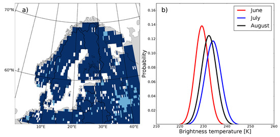
Figure 1.
(a) Shapiro-Wilk test for normality of the distribution shown for July. Dark blue regions null-hypothesis is not rejected, i.e., the data appears to be normally distributed. Light blue regions null-hypothesis is rejected, and white regions (over land) had too few years of data for testing. (b) Example PDFs of the fitted brightness temperature for boreal summmer months, June (red), July (blue) and August (black) for the grid-cell covering N and E.
The Gaussian fit to the for June (red), July (blue) and August (black) are shown for one grid-cell ( N and E) in Figure 1 b). The distributions show that June has a lower mean than July and August, with July being on average the warmest. The drought index value is computed by integrating the PDFs over . The integral is approximated by a summation up to the value of interest.
3.1.2. Temporal and Spatial Patterns of the Drought Indices
Figure 2 shows time-series of the SPI-1 (blue), STBI_SMOS (cyan), SSI_LDAS (red) and SSI_ESA_CCI (mangenta) over a grid-cell in Sweden ( N and E) (a) and Norway ( N and E) (b) from 2010 until 2018 for the boreal summer months, June, July and August. The two regions were selected to represent a region with and without the SSI_ESA_CCI data, and therefore show how the STBI_SMOS can represent regions where SM retrievals are masked. Furthermore, these two regions were affected by the 2018 summer drought, as seen from the negative anomalies in the indices for 2018.
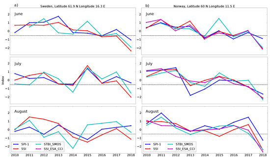
Figure 2.
(a) Time-series of the SPI-1 (blue), STBI_SMOS (cyan) and SSI_LDAS (red) over a grid-cell in Sweden ( N and E) from 2010 until 2018 for the boreal summer months June, July and August. The horizontal black dotted line indicate D0 drought conditions, see text for further explanation. Please note that for this region there were no observations for the computation of the SSI_ESA_CCI. (b) Same as a) but for a grid-cell in Norway ( N and E), here observations from the ESA CCI were available for the computation of the SSI_ESA_CCI drought index. For the different indices the grid-cell sizes are: for the STBI_SMOS and for the SPI-1, SSI_LDAS and SSI_ESA_CCI
Depending on the severity, a drought can be classified into a drought scale or D-scale, detailed explanation of this scale is provided in [3], see their Table 1. In this classification an SSI below is defined as being abnormally dry, and corresponding to a probability of occurrence. The D0 value as described in [3] is the lowest on the drought scale ranging from D0 to D4, where D1 is a moderate drought and D4 is described as an exceptional drought. Following [42], we use the D0 as a drought onset threshold, we see that for the regions in Figure 2a,b, severe drought conditions (see 2018 summer) is captured by the STBI_SMOS. The STBI_SMOS does not only capture dry events, it also captures years where a month is wetter than normal (index larger than zero). However, for positive index anomalies there seems to be more false events (e.g., June 2015 in Sweden, and June 2015 in Norway) than for the dry events.
We evaluate how well the STBI_SMOS, SSI_ESA_CCI and SPI-1 could capture the temporal dynamics of the SM drought by computing the correlation coefficients between the SSI_LDAS and the other metrics (STBI_SMOS, SSI_ESA_CCI and SPI-1). The LDAS-Monde index is then used as the reference index. This is justified by the fact that it incorporates both model and observation data in a data assimilation system. Other studies have shown that land data assimilation systems are able to correct for errors in precipitation datasets, and as a result, improve the representation of SSM (see for example [45]). Another example is provided by [46], where the authors show that the LDAS-Monde improves the representation of the 2012 US corn belt drought. We do not claim that the LDAS-Monde based data are superior to the other sources of data over this region. However, because of its use of state-of-the-art atmospheric forcing from ERA-5 and by combining SSM and LAI from satellites with model derived SSM and LAI it should be better than comparing with a model alone or to the satellite observations alone. It is also the best we can do for providing an independent reference index with a spatial scale close to that of the satellites.
In the computation of the correlation coefficient, we used June, July and August (boreal summer) data together from 2010 until 2018 to increase the number of data-points. The domain average was only computed for grid-cells where the Pearson correlation value was statistically significant at the level. Figure 3a shows the Pearson correlation coefficient between the STBI_SMOS and SSI_LDAS, regions with no values (grey regions over land) had a correlation not different from zero at the significance level. Most of the domain has a high correlation, except regions in south central Norway and from mid-Norway to northern Norway. In Figure 3b the Pearson correlation coefficient between the SSI_ESA_CCI and SSI_LDAS is shown. Here large regions in the Nordic countries (Norway, Sweden and Finland) have non significant correlation. This is likely because the SSI_ESA_CCI index has large regions with missing data for the individual months, thus resulting in a non-significant correlation and discarded values (grey regions in Figure 3). Summary statistics for the spatial correlations are shown in Table 2.
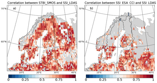
Figure 3.
(a) Pearson correlation coefficient between the STBI_SMOS and SSI_LDAS, red regions indicate a high positive correlation, masked (grey) regions have a correlation not significantly different from zero. (b) Same as a) but for the Pearson correlation between the SSI_ESA_CCI and SSI_LDAS.
Table 2.
Pearson R correlation coefficient between the SSI_LDAS and the, STBI_SMOS, SSI_ESA_CCI and the SPI-1. Computed for individual grid-cells (27 datapoints) and summed over the whole domain (all columns) and over grid-cells with overlap between all datasets (overlap columns). N indicates grid-cells with statistically significant correlation at the level, total number of land grid-cells were 2997.
The STBI_SMOS has a correlation with the SSI_LDAS of , it also has the highest number of grid-cells with a statistically significant correlation value ( out of 2997 grid-cells ()). The SSI_ESA_CCI index had a correlation of with the SSI_LDAS index, and significant values in out of 2997 () grid-cells. Finally, the SPI-1 correlation with SSI_LDAS was for out of 2997 () grid-cells. The high correlation between the STBI_SMOS and the SSI_LDAS indicate that the STBI_SMOS is able to capture the variability in the SM over the Nordic region as good as the SSI_ESA_CCI index. The number of grid-cells with statistically significant correlation values are higher for the STBI_SMOS than for the SSI_ESA_CCI, hence it provides better spatial coverage than the satellite derived SM index. To check that the high-correlation is not only found in regions where the SSI_ESA_CCI data were missing, we also compute the correlation for grid-cells covered by both products, see Table 2. Here the mean correlation is only taken for grid-cells where we have data for all the four indices (resulting in 800 of 2997 land grid-cells being covered, i.e., ).
3.2. Case Study of the Summer 2018 Drought
To further evaluate the performance of the STBI for drought mapping we utilized the 2018 summer drought over the Nordic countries as a case study.
3.2.1. Comparison between the STBI_SMOS, SSI_LDAS, SSI_ESA_CCI, SPI-1 and SSI_SMOS
The limited number of reliable satellite derived SM observations in the SMOS-L2 (Figure 4q–t) and ESA CCI COMBINED product (Figure 4i–l) motivated our attempt to describe the 2018 Nordic drought using the observed brightness temperature (). In addition to the poor coverage, the Standardized Soil moisture Index for SMOS (SSI_SMOS) exhibits noisy patterns, and little resemblance to the SSI_LDAS in Figure 4. Comparing the STBI in Figure 4a–d) to the SSI_ESA_CCI in Figure 4i–l) we see that the STBI_SMOS has a better spatial coverage than the SSI_ESA_CCI. Large regions over Sweden and northern Finland are not covered by the SSI_ESA_CCI. This problem is addressed by using the data.
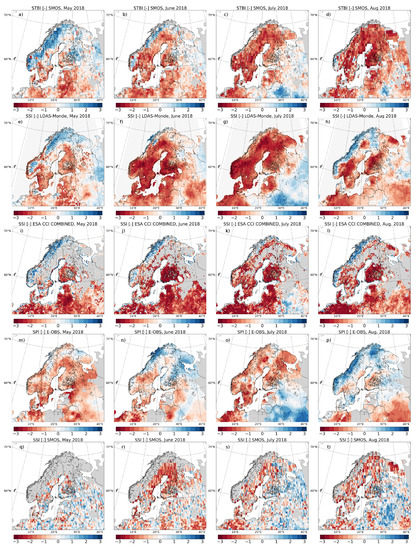
Figure 4.
Drought indices, blue/red is above/below average precipitation, or soil moisture. Grey colour indicates regions without data. Columns from left to right are for May, June, July and August. (a–d) Standardized microwave Brightness Temperature Index (STBI_SMOS). (e–h) Standardized Soil moisture Index (SSI_LDAS). (i–l) Standardized Soil moisture Index ESA CCI (SSI_ESA_CCI). (m–p) Standardized Precipitation Index (SPI-1). (q–t) Standardized Soil moisture Index SMOS (SSI_SMOS).
Figure 4a,e,i,m,q show the STBI_SMOS, SSI_LDAS, SSI_ESA_CCI, SPI-1 and SSI_SMOS for May 2018 over the Nordic region. The SPI-1 indicates a precipitation deficit for most of the domain. The STBI_SMOS, SSI_LDAS and SSI_ESA_CCI show that northern parts of Norway and the mountain regions in the south of Norway are wetter (colder for the STBI) than usual. This signal might come from late snowmelt wetting the soil in the northern latitudes and the mountainous regions in southern Norway. We also note that southern parts of Sweden and Finland are drier (warmer) than usual for the STBI_SMOS, SSI_LDAS and SSI_ESA_CCI. In general, the spatial patterns for May are very similar for the STBI and SSI_LDAS, although the STBI overestimates the wet regions in northern Norway and in Finland.
Next we examine the indices during June 2018. Figure 4b,f,j,n,r show the STBI_SMOS, SSI_LDAS, SSI_ESA_CCI, SPI-1 and SSI_SMOS, respectively. The dry conditions seen in the SPI-1 continue in eastern Norway, southern Sweden and Denmark. Northern parts of Norway and most of Finland experience rainy conditions seen from the SPI-1. Eastern Norway, Sweden, Finland, Denmark and the Baltic countries have a dry anomaly in the STBI_SMOS, SSI_LDAS and SSI_ESA_CCI. Northern parts of Sweden and Finland have missing values for the SSI_ESA_CCI index; however, the STBI_SMOS shows similar patterns as the SSI_LDAS, except for the wet regions in southwestern and northern Norway. When comparing the STBI_SMOS to the SSI_LDAS we see that the STBI_SMOS captures the wet (cold) regions in the east of the domain. The reason why the STBI is able to capture wet/dry anomalies is because of its close relationship to SSM. This is why L-band radiometers are used for SM retrievals in the first place. The large difference in dielectric constant between water (∼80) and dry soil (∼3), results in a large range in the emissivity of the soil, and therefore also the soil brightness temperature [47]. Low/high brightness temperature indicates that the surface is wet/dry. The STBI can therefore also detect wet anomalies (such as water ponding on the surface), which can be useful in monitoring flood and/or heavy precipitation events. Typically, for heavy precipitation events where you get water ponding on the surface, the SM retrieval does not make any sense, and the retrieval is omitted [16].
In July in Figure 4c,g,k,o,s the SPI-1 shows a dry anomaly for Norway, Sweden, Finland and Denmark. In July, drought conditions were dominant over most of the domain, except for regions in the south central and east, which is reflected in all of the indices. Again, there are gaps in the SSI_ESA_CCI over large regions of Sweden and Finland. These gaps are not present in the STBI_SMOS, which is consistent with the SSI_LDAS, showing dry anomalies for this region. Close to normal conditions in northern parts of Poland are found for both the STBI_SMOS and the SSI_LDAS for July; this is not seen for the SSI_ESA_CCI.
In August most of Norway experienced wetter than usual conditions (seen from the SPI-1), this is reflected in the SSI_ESA_CCI and the SSI_LDAS, but not in the STBI_SMOS, see Figure 4d,h,l,p. One reason for this could be precipitation intercepted by the vegetation, increasing the VWC, again increasing the emissivity from the vegetation [18]. Higher emissivity from a recovering vegetation could therefore mask out precipitation events and cause a false drought signal, as seen in August 2018. We see this as an argument for simultaneously retrieving SSM and VOD, as applying a constant (in time) VOD value would likely cause the SSM retrieval to be drier than expected because of the increased Tb from the vegetation.
The SPI-1, SSI_LDAS and SSI_ESA_CCI are all on the same spatial scale (∼25 km), however the STBI_SMOS is posted on a coarser (∼36 km) grid. In Figure 2 we plotted the time-series of the grid-cell closest to the given latitude/longitude, and despite the spatial mismatch between the STBI and the other indices, we see that there is a good temporal agreement which is also reflected in the Pearson correlation coefficient in Table 2. Droughts are by nature large scale events (as seen in Figure 4), thus a small spatial mismatch between our indices should not alter our conclusions on the spatial patterns of the drought.
3.2.2. Drought Severity
Following the D-scale [3], an SSI below is defined as a severe drought (D2 conditions). In Figure 5 we have plotted the STBI_SMOS (a–d), SSI_LDAS (e–h), SSI_ESA_CCI (i–l) and SPI-1 (m–p) for D2 conditions for May, June, July and August in 2018. We have not included the SSI_SMOS in Figure 5, because from Figure 4q–t we saw that the SMOS SM data were noisy and had large spatial gaps. The difference between the one month land surface indices (STBI_SMOS, SSI_LDAS and SSI_ESA_CCI) and the SPI-1 is most likely due to the lag time between the meteorological drought (one month SPI) and the agricultural drought (one month SSI). The SPI-1 has a shorter memory than the SSI, hence a dry SPI-1 in month i is often followed by a dry SSI in month , even though the precipitation is back to normal conditions in month . Using the SSI_LDAS as a reference we see that the STBI_SMOS is able to capture regions in severe drought where the SSI_ESA_CCI has masked values from the retrieval. This can be seen in southern Norway (July) and northern and central Sweden (July). Comparing Figure 5c,g,k we see that northern parts of Poland do not have severe drought conditions for the SSI_LDAS, and this is captured by the STBI_SMOS but not by the SSI_ESA_CCI. On the other hand, the spatial pattern of the SSI_ESA_CCI drought severity in June has better agreement with the SSI_LDAS than the comparison of the STBI_SMOS versus the SSI_LDAS. In August, the STBI_SMOS (Figure 2d)) is overestimating the regions experiencing severe drought conditions in northern Norway and Sweden, when compared to the SSI_LDAS (Figure 5h)).
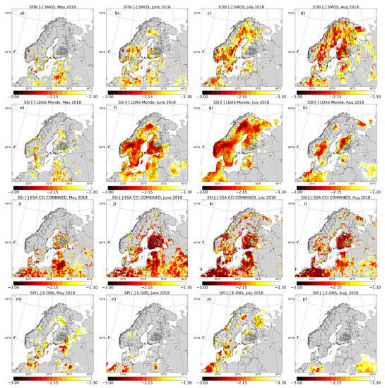
Figure 5.
Regions with severe drought conditions, drought index < for May, June, July and August. Red regions are severe drought conditions, while yellow and white are regions with less severe drought conditions. Grey colour indicates regions where the drought indices are larger than . (a–d) STBI <. (e–h) SSI_LDAS <. (i–l) SSI_ESA_CCI <. (m–p) SPI-1 <.
3.2.3. Drought Onset and Recovery
Accurate monitoring of drought onset and recovery could help farmers and decision makers minimize the negative impacts of a drought. Here we evaluate the temporal evolution of the STBI_SMOS index against the temporal evolution of the SSI_LDAS SSI_ESA_CCI and SPI-1 during the 2018 summer drought. As a consequence of the drought several regions in the Nordic countries experienced wildfires and agricultural losses [8,48], here we have chosen three sites to represent such conditions. In Figure 6 we have selected grid-cells in the vicinity of (a) Jokkmokk municipality, Sweden, (b) Tovaasen, Sweden and (c) Nes in Akershus municipality, Norway. These regions experienced large wildfires and agricultural droughts during the summer 2018 heatwave [6,7,8,48]. The horizontal dotted black line shows the D0 condition (moderate drought). The first thing to note is that in Figure 6a,b there are no data for the SSI_ESA because these grid locations are flagged in the retrieval algorithm. This limits the use of the SSI_ESA_CCI over regions in the Nordic countries for drought monitoring and mapping. Hence a reason for choosing grid-cells where we have no SSI_ESA_CCI data is to show that the STBI_SMOS can be used to monitor the drought in these regions.
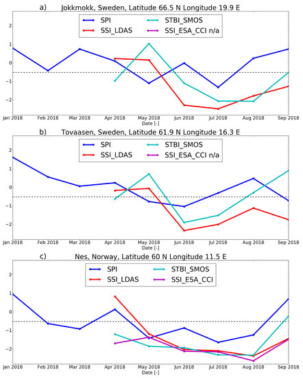
Figure 6.
SPI-1 (blue), SSI_LDAS (red), STBI_SMOS (cyan) and SSI_ESA_CCI (magenta) time series.Black dotted horizontal line indicate D0 drought conditions. (a) Jokkmokk municipality, Sweden, (b) Tovaasen, Sweden, (c) Nes in Akershus municipality, Norway. Latitudes are given in degrees north (N) and longitudes are given in degrees east (E).
The Jokkmokk municipality lies above the Arctic circle in northern Sweden and it experienced large wildfires during the 2018 summer. In Figure 6a we see that the precipitation deficit (low SPI-1) starting in May causes the STBI_SMOS (cyan) and SSI_LDAS (red) to fall below D0 conditions in June. The close to normal SPI-1 conditions in June has little impact on the land surface indices (STBI_SMOS and SSI_LDAS). Precipitation deficit in July and only close to normal SPI-1 conditions in August and September, results in a slow recovery of the land surface indices for the Jokkmokk site.
Tovaasen lies in the Ljusdalen municipality, a region in Sweden which experienced large wildfires in mid-July 2018. In Figure 6b we see that the SPI-1 (blue) is close to normal for February, March and April. In May and June the precipitation deficit leads to a decrease in the STBI_SMOS (cyan) and SSI_LDAS (red). In August the SPI-1 is close to normal conditions, but this is not enough for the STBI_SMOS and SSI_LDAS to recover. In September the STBI_SMOS and the SSI_LDAS diverges, with the STBI_SMOS showing drought recovery while the SSI_LDAS more closely follows the SPI-1 and shows drought conditions.
Much of the agriculture in Norway lies in the south-eastern parts of the country and here we choose a grid-cell which covers Nes in Akershus municipality. In Figure 6c we see that low SPI-1 conditions in the February and March likely caused abnormally dry (warm) conditions in April for the STBI_SMOS (cyan) and SSI_ESA_CCI (magenta). The continued precipitation deficit in May, June and July was propagated into the land seen by the low STBI_SMOS, SSI_LDAS and SSI_ESA_CCI. Here the three land surface drough indices follow each other closely during the dry spell in May, June, July and August.
The case study for the 2018 summer show that the STBI_SMOS has potential to supplement information to drought monitoring over the Nordic region. In particular, we see that it was able to monitor the drought in regions where data from the SM retrievals were missing. The STBI_SMOS did however miss the transition to a wet anomaly for large regions in Norway in August 2018 (Figure 4d).
4. Conclusions
In this study, we outlined a new approach for directly applying passive microwave brightness temperature to monitor and map drought over the Nordic countries. We propose a standardized index (STBI) based on passive microwave brightness temperature data. The rationale behind this choice is that the convolves information about soil moisture, soil temperature and vegetation water content, which are all important factors in drought and flood monitoring. The brightness temperature also provides a better spatial and temporal coverage than the retrieved soil moisture, because we avoid the retrieval problem, which is problematic over northern latitudes owing to dense vegetation, strong topography, high water fraction and snow cover. The brightness temperature is also available earlier than than the retrieved soil moisture, which will benefit the drought monitoring capabilities of the index.
We found that the STBI_SMOS metric was able to capture the spatial patterns of the 2018 Nordic drought, especially for the very dry conditions seen in July 2018, when comparing it to the SSI from LDAS-Monde. As seen for two test sites in Sweden and one in Norway, the STBI_SMOS drought onset and end were in line with the SSI_LDAS and SPI-1. The STBI_SMOS was also characterized by a one month lag compared to the SPI-1 (as often seen in land surface drought metrics [19]), indicating that it contained information about soil/vegetation moisture, and not only about land surface temperature. One criticism of the index is that it did not capture the drought end/recovery seen in August 2018 for our case study. This is likely linked to the fact that when the vegetation recovers from drought the VWC increases resulting in an increase of Tb [18]. We therefore stress that the index should be used as a supplement to other monitoring tools, and not as a replacement.
The results from this work show that passive microwave observations (in the L-band) could be implemented in a Nordic drought monitoring system. We expect that the STBI could be a supplement to modelling tools, and that downscaling of the index would enhance its applicability for drought monitoring at decision making scales. In the future it would be possible to calculate the STBI for observations from more recently launched L-band satellites, such as the SMAP NASA mission [24]. The performance of passive microwave observations in the C-band should also be investigated for drought monitoring over northern latitudes because the temporal span of these missions are longer than the L-band missions, and hence a more reliable estimate of the () climatology can be computed. The method could also be expanded to other regions of the world, where retrieval of soil moisture is difficult. In addition, to fully investigate the advantages of the STBI future work should consider computing the STBI over regions where we know that the SM retrieval is better understood. This study was also the first attempt to monitor agricultural drought over the Nordic region from space and compare the skill of a space based drought index with that of a state-of-the-art land surface data assimilation system (LDAS-Monde). We expect that future development of the STBI_SMOS metric could benefit farmers, decision makers and others depending on information concerning agricultural drought over the Nordic countries.
Author Contributions
J.B., P.D.H., W.A.L., C.A. and P.S. conceived and designed the study. C.A. designed and ran the land surface data assimilation system. J.B. did the analysis and wrote the manuscript. All authors provided comments on the manuscript.
Funding
The main author is supported by the Research Council of Norway (NFR PhD-grant 239947, 2015–2019).
Acknowledgments
The corresponding author would like to dedicate this paper to the memory of William A. Lahoz. The corresponding author would also like to thank Laurent Bertino for helpful comments in the preparation of this paper. The authors would like to thank the Copernicus Global Land Service for providing the satellite-derived LAI products and soil moisture for the LDAS-Monde assimilation. We would also like to thank the Copernicus Climate Change Service (C3S) for providing the ESA CCI COMBINED soil moisture data, and the ERA-5 data used for atmospheric forcing in the LDAS-Monde system. We acknowledge the E-OBS dataset from the EU-FP6 project ENSEMBLES (http://ensembles-eu.metoffice.com) and the data providers in the ECAD project (http://www.ecad.eu). The SMOS data are available online from ESA. The Copernicus Climate Change soil moisture data are available at https://cds.climate.copernicus.eu. The LDAS-Monde derived data and analysis scripts can be accessed at ftp://ftp.nilu.no/Pub/nilu/jostein/Data/. Finally, we would like to thank the reviewers for their comments on the paper.
Conflicts of Interest
The authors declare no conflict of interest.
References
- Gerber, N.; Mirzabaev, A. Benefits of Action and Costs of Inaction: Drought Mitigation and Preparedness—A Literature Review; Technical report; World Meteorological Organization (WMO) and Global Water Partnership (GWP): Geneva, Switzerland; Stockholm, Sweden, 2017. [Google Scholar]
- Emmer, A. Geographies and Scientometrics of Research on Natural Hazards. Geosciences 2018, 8, 382. [Google Scholar] [CrossRef]
- Svoboda, M. Drought Monitor. Bull. Am. Meteorol. Soc. 2002, 83, 1181–1190. [Google Scholar] [CrossRef]
- Luo, L.; Wood, E.F. Monitoring and predicting the 2007 U.S. drought. Geophys. Res. Lett. 2007, 34. [Google Scholar] [CrossRef]
- Lentze, G. Newsletter No. 157—Autumn 2018. ECMWF Newsletter. 2018. Available online: https://www.ecmwf.int/node/18705 (accessed on 19 May 2019).
- WMO. The State of the Global Climate in 2018; Technical Report; World Meteorological Organization: Geneva, Switzerland, 2018; Available online: https://public.wmo.int/en/our-mandate/climate/wmo-statement-state-of-global-climate (accessed on 19 May 2019).
- Landbruksdirektoratet. Available online: https://www.landbruksdirektoratet.no/no/statistikk/landbrukserstatning/klimarelaterte-skader-og-tap/avlingssvikt (accessed on 28 March 2019).
- Skaland, R.G.; Colleuille, H.; Andersen, A.S.H.; Mamen, J.; Grinde, L.; Tajet, H.T.T.; Lundstad, E.; Sidselrud, L.F.; Tunheim, K.; Hanssen-Bauer, I.; et al. Tørkesommeren 2018; Technical Report; The Norwegian Meteorological Institute: Oslo, Norway, 2019; Available online: https://fido.nrk.no/cccfcb66f38035154dd25ba51c2573ae231d397583bee2a4e545ae0b6e3fc2dd/Torkesommeren%2018__.pdf (accessed on 19 May 2019).
- Liberto, T.D. A Hot, Dry Summer Has Led to Drought in Europe in 2018. Available online: https://www.climate.gov/news-features/event-tracker/hot-dry-summer-has-led-drought-europe-2018 (accessed on 19 May 2019).
- Samaniego, L.; Thober, S.; Kumar, R.; Wanders, N.; Rakovec, O.; Pan, M.; Zink, J.; Sheffield, E.; Wood, E.F.; Marx, A. Anthropogenic warming exacerbates European soil moisture droughts. Nat. Clim. Chang. 2018, 8, 421–426. [Google Scholar] [CrossRef]
- Trenberth, K.E.; Dai, A.; Van Der Schrier, G.; Jones, P.D.; Barichivich, J.; Briffa, K.R.; Sheffield, J. Global warming and changes in drought. Nat. Clim. Chang. 2014, 4, 17–22. [Google Scholar] [CrossRef]
- Greve, P.; Gudmundsson, L.; Seneviratne, S.I. Regional scaling of annual mean precipitation and water availability with global temperature change. Earth Syst. Dyn. 2018, 9, 227–240. [Google Scholar] [CrossRef]
- Mu, Q.; Zhao, M.; Kimball, J.S.; McDowell, N.G.; Running, S.W. A remotely sensed global terrestrial drought severity index. Bull. Am. Meteorol. Soc. 2013, 94, 83–98. [Google Scholar] [CrossRef]
- AghaKouchak, A.; Farahmand, A.; Melton, F.S.; Teixeira, J.; Anderson, M.C.; Wardlow, B.D.; Hain, C.R. Remote sensing of drought: Progress, challenges and opportunities. Rev. Geophys. 2015, 53. [Google Scholar] [CrossRef]
- Sadri, S.; Wood, E.F.; Pan, M. Developing a drought-monitoring index for the contiguous US using SMAP. Hydrol. Earth Syst. Sci. 2018, 22, 6611–6626. [Google Scholar] [CrossRef]
- Kerr, Y.H.; Waldteufel, P.; Richaume, P.; Wigneron, J.P.; Ferrazzoli, P.; Mahmoodi, A.; Al Bitar, A.; Cabot, F.; Gruhier, C.; Juglea, S.E.; et al. The SMOS soil moisture retrieval algorithm. IEEE Trans. Geosci. Remote Sens. 2012, 50, 1384–1403. [Google Scholar] [CrossRef]
- Fernandez-Moran, R.; Al-Yaari, A.; Mialon, A.; Mahmoodi, A.; Al Bitar, A.; De Lannoy, G.; Rodriguez-Fernandez, N.; Lopez-Baeza, E.; Kerr, Y.; Wigneron, J.-P. SMOS-IC: An alternative SMOS soil moisture and vegetation optical depth product. Remote Sens. 2017, 9, 457. [Google Scholar] [CrossRef]
- Jones, A.S.; Vukićević, T.; Vonder Haar, T.H. A Microwave Satellite Observational Operator for Variational Data Assimilation of Soil Moisture. J. Hydrometeorol. 2004, 5, 213–229. [Google Scholar] [CrossRef]
- Sheffield, J.; Goteti, G.; Wen, F.; Wood, E.F. A simulated soil moisture based drought analysis for the United States. J. Geophys. Res. D Atmos. 2004, 109, 1–19. [Google Scholar] [CrossRef]
- Yuan, X.; Ma, Z.; Pan, M.; Shi, C. Microwave remote sensing of short-term droughts during crop growing seasons. Geophys. Res. Lett. 2015, 42, 4394–4401. [Google Scholar] [CrossRef]
- ESA. ESA SMOS Online Dissemination Service. Available online: https://smos-diss.eo.esa.int/oads/access/ (accessed on 19 May 2019).
- Wigneron, J.P.; Kerr, Y.; Waldteufel, P.; Saleh, K.; Escorihuela, M.J.; Richaume, P.; Ferrazzoli, P.; de Rosnay, P.; Gurney, R.; Calvet, J.C.; et al. L-band Microwave Emission of the Biosphere (L-MEB) Model: Description and calibration against experimental data sets over crop fields. Remote Sens. Environ. 2007, 107, 639–655. [Google Scholar] [CrossRef]
- Njoku, E.G.; Wilson, W.J.; Yueh, S.H.; Dinardo, S.J.; Li, F.K.; Jackson, T.J.; Lakshmi, V.; Bolten, J. Observations of soil moisture using a passive and active low-frequency microwave airborne sensor during SGP99. IEEE Trans. Geosci. Remote Sens. 2002, 40, 2659–2673. [Google Scholar] [CrossRef]
- Entekhabi, D.; Njoku, E.G.; O’Neill, P.E.; Kellogg, K.H.; Crow, W.T.; Edelstein, W.N.; Entin, J.K.; Goodman, S.D.; Jackson, T.J.; Johnson, J.; et al. The soil moisture active passive (SMAP) mission. Proc. IEEE 2010, 98, 704–716. [Google Scholar] [CrossRef]
- De Rosnay, P.; Drusch, M.; Boone, A.; Balsamo, G.; Decharme, B.; Harris, P.; Kerr, Y.; Pellarin, T.; Polcher, J.; Wigneron, J.-P. AMMA land surface model intercomparison experiment coupled to the community microwave emission model: ALMIP-MEM. J. Geophys. Res. Atmos. 2009, 114. [Google Scholar] [CrossRef]
- Drusch, M.; Holmes, T.; de Rosnay, P.; Balsamo, G. Comparing ERA-40-Based L-Band Brightness Temperatures with Skylab Observations: A Calibration/Validation Study Using the Community Microwave Emission Model. J. Hydrometeorol. 2009, 10, 213–226. [Google Scholar] [CrossRef]
- De Lannoy, G.J.; Reichle, R.H. Assimilation of SMOS brightness temperatures or soil moisture retrievals into a land surface model. Hydrol. Earth Syst. Sci. 2016, 20, 4895–4911. [Google Scholar] [CrossRef]
- Dorigo, W.; Gruber, A.; De Jeu, R.A.; Wagner, W.; Stacke, T.; Loew, A.; Albergel, C.; Brocca, L.; Chung, D.; Parinussa, R.M.; et al. Evaluation of the ESA CCI soil moisture product using ground-based observations. Remote Sens. Environ. 2015, 162, 380–395. [Google Scholar] [CrossRef]
- Dorigo, W.; Wagner, W.; Albergel, C.; Albrecht, F.; Balsamo, G.; Brocca, L.; Chung, D.; Ertl, M.; Forkel, M.; Gruber, A.; et al. ESA CCI Soil Moisture for improved Earth system understanding: State-of-the art and future directions. Remote Sens. Environ. 2017, 203, 185–215. [Google Scholar] [CrossRef]
- Scanlon, T.; Chung, D.; Paulik, C.; Kidd, R. Product User Guide and Specification; Technical Report; ECMWF: Reading, UK, 2018; Available online: http://datastore.copernicus-climate.eu/c3s/published-forms/c3sprod/satellite-soil-moisture/product-user-guide-v2.3.pdf (accessed on 19 May 2019).
- Haylock, M.R.; Hofstra, N.; Klein Tank, A.M.G.; Klok, E.J.; Jones, P.D.; New, M. A European daily high-resolution gridded dataset of surface temperature and precipitation. J. Geophys. Res. Atmos. 2008, 113, D20119. [Google Scholar] [CrossRef]
- Albergel, C.; Munier, S.; Leroux, J.D.; Dewaele, H.; Fairbairn, D.; Lavinia Barbu, A.; Gelati, E.; Dorigo, W.; Faroux, S.; Meurey, C.; et al. Sequential assimilation of satellite-derived vegetation and soil moisture products using SURFEX-v8.0: LDAS-Monde assessment over the Euro-Mediterranean area. Geosci. Model Dev. 2017, 10, 3889–3912. [Google Scholar] [CrossRef]
- Albergel, C.; Dutra, E.; Bonan, B.; Zheng, Y.; Munier, S.; Balsamo, G.; de Rosnay, P.; Muñoz-Sabater, J.; Calvet, J.C. Monitoring and Forecasting the Impact of the 2018 Summer Heatwave on Vegetation. Remote Sens. 2019, 11, 520. [Google Scholar] [CrossRef]
- Noilhan, J.; Mahfouf, J.F. The ISBA land surface parameterisation scheme. Glob. Planet. Chang. 1996, 13, 145–159. [Google Scholar] [CrossRef]
- Calvet, J.C.; Noilhan, J.; Roujean, J.L.; Bessemoulin, P.; Cabelguenne, M.; Olioso, A.; Wigneron, J.P. An interactive vegetation SVAT model tested against data from six contrasting sites. Agric. For. Meteorol. 1998, 92, 73–95. [Google Scholar] [CrossRef]
- Masson, V.; Le Moigne, P.; Martin, E.; Faroux, S.; Alias, A.; Alkama, R.; Belamari, S.; Barbu, A.; Boone, A.; Bouyssel, F.; et al. The SURFEXv7.2 land and ocean surface platform for coupled or offline simulation of earth surface variables and fluxes. Geosci. Model Dev. 2013, 6, 929–960. [Google Scholar] [CrossRef]
- Mahfouf, J.F.; Bergaoui, K.; Draper, C.; Bouyssel, F.; Taillefer, F.; Taseva, L. A comparison of two off-line soil analysis schemes for assimilation of screen level observations. J. Geophys. Res. Atmos. 2009, 114. [Google Scholar] [CrossRef]
- Albergel, C.; Calvet, J.C.; Mahfouf, J.F.; Rüdiger, C.; Barbu, A.L.; Lafont, S.; Roujean, J.-L.; Walker, J.P.; Crapeau, M.; Wigneron, J.-P. Monitoring of water and carbon fluxes using a land data assimilation system: A case study for southwestern France. Hydrol. Earth Syst. Sci. 2010, 14, 1109–1124. [Google Scholar] [CrossRef]
- Barbu, A.L.; Calvet, J.C.; Mahfouf, J.F.; Albergel, C.; Lafont, S. Assimilation of Soil Wetness Index and Leaf Area Index into the ISBA-A-gs land surface model: Grassland case study. Biogeosciences 2011, 8, 1971–1986. [Google Scholar] [CrossRef]
- De Rosnay, P.; Drusch, M.; Vasiljevic, D.; Balsamo, G.; Albergel, C.; Isaksen, L. A simplified extended kalman filter for the global operational soil moisture analysis at ECMWF. Q. J. R. Meteorol. Soc. 2013, 139, 1199–1213. [Google Scholar] [CrossRef]
- Wilks, D.S. Statistical Methods in Atmospheric Sciences; Academic Press: Cambridge, MA, USA, 2005; Volume 100, p. 676. [Google Scholar]
- Farahmand, A.; AghaKouchak, A.; Teixeira, J. A vantage from space can detect earlier drought onset: An approach using relative humidity. Sci. Rep. 2015, 5. [Google Scholar] [CrossRef] [PubMed]
- Farahmand, A.; AghaKouchak, A. A generalized framework for deriving nonparametric standardized drought indicators. Adv. Water Resour. 2015, 76, 140–145. [Google Scholar] [CrossRef]
- Gringorten, I.I. A plotting rule for extreme probability paper. J. Geophys. Res. 1963, 68, 813–814. [Google Scholar] [CrossRef]
- Blyverket, J.; Hamer, P.D.; Bertino, L.; Albergel, C.; Fairbairn, D.; Lahoz, W.A. An Evaluation of the EnKF vs. EnOI and the Assimilation of SMAP, SMOS and ESA CCI Soil Moisture Data over the Contiguous US. Remote Sens. 2019, 11, 478. [Google Scholar] [CrossRef]
- Albergel, C.; Munier, S.; Bocher, A.; Bonan, B.; Zheng, Y.; Draper, C.; Leroux, D.J.; Calvet, J.C. LDAS-Monde sequential assimilation of satellite derived observations applied to the contiguous US: An ERA-5 driven reanalysis of the land surface variables. Remote Sens. 2018, 10, 1627. [Google Scholar] [CrossRef]
- Njoku, E.G.; Entekhabi, D. Passive microwave remote sensing of soil moisture. J. Hydrol. 1996, 184, 101–129. [Google Scholar] [CrossRef]
- Watts, J. The Swedish Town on the Frontline of the Arctic Wildfires. 2018. Available online: https://www.theguardian.com/world/2018/jul/30/the-swedish-town-on-the-frontline-of-the-arctic-wildfires (accessed on 7 February 2019).
© 2019 by the authors. Licensee MDPI, Basel, Switzerland. This article is an open access article distributed under the terms and conditions of the Creative Commons Attribution (CC BY) license (http://creativecommons.org/licenses/by/4.0/).