Article

Evaluating the Potential of Multi-Seasonal CBERS-04 Imagery for Mapping the Quasi-Circular Vegetation Patches in the Yellow River Delta Using Random Forest

1
State Key Laboratory of Resources and Environmental Information System, Institute of Geographic Sciences and Natural Resources Research, Chinese Academy of Sciences, Beijing 100101, China
2
Jiangsu Center for Collaborative Innovation in Geographical Information Resource Development and Application, Nanjing 210023, China
3
Henan Aero Geophysical Survey and Remote Sensing Center, Zhengzhou 450053, China
*
Author to whom correspondence should be addressed.
Remote Sens. 2019, 11(10), 1216; https://doi.org/10.3390/rs11101216
Submission received: 26 March 2019 / Revised: 17 May 2019 / Accepted: 18 May 2019 / Published: 22 May 2019

Abstract

:
High-resolution satellite imagery enables decametric-scale quasi-circular vegetation patch (QVP) mapping, which greatly aids the monitoring of vegetation restoration projects and the development of theories in pattern evolution and maintenance research. This study analyzed the potential of employing five seasonal fused 5 m spatial resolution CBERS-04 satellite images to map QVPs in the Yellow River Delta, China, using the Random Forest (RF) classifier. The classification accuracies corresponding to individual and multi-season combined images were compared to understand the seasonal effect and the importance of optimal image timing and acquisition frequency for QVP mapping. For classification based on single season imagery, the early spring March imagery, with an overall accuracy (OA) of 98.1%, was proven to be more adequate than the other four individual seasonal images. The early spring (March) and winter (December) combined dataset produced the most accurate QVP detection results, with a precision rate of 66.3%, a recall rate of 43.9%, and an F measure of 0.528. For larger study areas, the gain in accuracy should be balanced against the increase in processing time and space when including the derived spectral indices in the RF classification model. Future research should focus on applying higher resolution imagery to QVP mapping.

1. Introduction

In arid and semi-arid regions of the world, vegetation usually appears as patches due to the environmental constraints such as a limited water supply, soil salinization or local microtopography. According to size, area and spatial distribution, vegetation patches are characterized as banded (i.e., tiger vegetation) or spotted (i.e., leopard vegetation) [1]. Compared with banded vegetation patterns, the spotted vegetation pattern has not as yet attracted equivalent attention [2]. Patchy vegetation patterns have been reported in America, Africa, Asia, Australia, and Spain [3,4,5,6,7,8,9,10,11,12,13,14,15,16], where the range of annual precipitation is from 50 to 750 mm, and appears to be unrelated to any particular soil type or plant species [14]. In general, it is considered as the result of plant-oil feedback occurring in water-limited regions [12,14,15,16]. Although there is an ongoing debate concerned with the mechanisms for the formation of patchy vegetation patterns, vegetation patchiness can generally increase primary production, influence biodiversity, affect surface runoff and soil erosion, and suggest key indices for ecosystem function and for the management of arid and semi-arid lands [1,16,17,18]. Mapping vegetation patches is, therefore, important for a better understanding of patch patterns, mechanisms for formation and evolution, and function. Moreover, such mapping can provide valuable information for the development of adaptive vegetation recovery and re-establishment strategies for increasingly degraded ecosystems in arid and semi-arid zones [19].
Remote sensing is an effective technology for the creation of vegetation maps. Due to the relatively small size, vegetation patch mapping most frequently involves the application of aerial photographs and high-resolution satellite images. Aerial photographs have long been recognized as an important data source for mapping patchy vegetation patterns since aerial photographs first became accessible in the early 1940s [2,20]. The circular patches (with an area of approximately <90 m2 to >3000 m2) of Spartina patens on Cox Island, Siuslaw Estuary, Oregon were mapped using sequential air photos (scale 1:1500) from 1939 to 1980 and their area determined by planimetry [9]. Vegetation patches (with spatial scales of 2–3 m) on the eastern flanks of Mt. Carmel were derived from orthorectified aerial photographs with a 75 cm pixel resolution using a Maximum Likelihood Classifier (MLC) [20]. The fairy circles (with an average diameter of 5–8 m) of Kaokoland, Namibia were detected from a set of aerial photographs (Scale 1:78,000) [21]. Two-dimensional wavelet combined with a 1 m aerial photograph was used to identify individual juniper trees (crown diameter of 2–9 m) and thereby to analyze the encroachment of juniper plants on to a sagebrush steppe landscape [22]. A set of historical aerial photographs have also been used to analyze the onset and trends of an invasion by Pteronia incana into the dry Karoo region of South Africa [19]. Multi-temporal aerial color infrared high-resolution images with a spatial resolution of 1 m were used to validate a distinct discrimination of Pteronia incana from other surfaces in an invaded area in Eastern Cape, South Africa [23]. Previous studies have proved that aerial photograph with a pixel size of 2 m are sufficient to study decametric-scale vegetation patch patterns [24,25]. With the launch of high spatial resolution civil commercial satellites in 1999, increasing numbers of studies have been carried out concerning the dynamics of vegetation patch patterns either by combining historical aerial photographs with multi-temporal high-resolution satellite images in recent years, or with the sole use of multi-temporal high-resolution satellite images. For example, a set of historical aerial photographs with a spatial resolution of 86 cm and a QuickBird satellite image with a spatial resolution of 60 cm were used to monitor shrub encroachment from 1937 to 2003 in southern New Mexico using the Object-Based Image Analysis method (OBIA), and approximately 87% of all shrubs of more than 2 m2 were identified [26]. Shekede et al. [25] used a discrete wavelet transform to map dynamics in the encroachment of woody patches (with an average diameter of between 8 m and 32 m) onto Zimbabwean savanna through the integration of multi-temporal aerial photographs (Scale 1:20,000) with the resample high spatial resolution (a spatial resolution of 2 m) GeoEye satellite images. High spatial resolution SPOT 5 (for which sharpened imagery has a spatial resolution of 2.5 m), QuickBird and IKONOS (with a spatial resolution of 80 cm) satellite imagery has been successfully used to map tree canopy cover patterns in savannas, and tree canopy sizes mapped with SPOT 5 imagery using the OBIA method had a similar distribution to those observed with QuickBird detection [27]. SPOT 5 (a spatial resolution of 2.5 m), ALOS (a spatial resolution of 2.5 m), ZY-3(a spatial resolution of 5.8 m), and QuickBird imagery have been also successfully used to detect the quasi-circular vegetation patches (QVPs, with an area of 115 m2 to more than 1200 m2) in the Yellow River Delta (YRD), China [28,29,30]. The WorldView-2 satellite imagery (with a spatial resolution of 2 m) was recognized as more appropriate for the mapping to be used for a global estimation of giant reed invasion [31].
The above-mentioned studies use single-date high-resolution imagery to map vegetation patches. Multi-date images are not generally used for the detection of such patches, but are mainly used to analyze the dynamics of vegetation patch patterns according to differences between the bi-temporal images. The phenological information for vegetation derived from multi-seasonal imagery is very useful for mapping tree species [32,33,34,35,36,37,38,39], forest cover [40,41,42], crop types [43,44,45,46,47,48,49], bush encroachment [25], grassland [50,51,52,53,54], and land use/land cover and changes [55,56,57,58,59,60,61,62]. Despite the different conclusions obtained from a few studies [36,63,64], generally, multi-spectral and seasonal imagery can largely support higher classification accuracy than single-date imagery. During the temporal series classification procedure, it is necessary to find the optimal number of images and the optimal seasonal composition periods for mapping the target research objects in a region [46,58,65], because the acquisition of a large number of images may not be feasible due to cloud contamination, the satellite revisiting cycle, the high price, and the fact that long image composition periods may be less informative and lead to information redundancy [43,48,66].
Temporal series approaches involve the pixel-based and OBIA classification using several algorithms: principal component analysis, multi-temporal tasseled cap transformation, ISODATA, K-Means, maximum likelihood classification, linear discriminant analysis, multinomial logistic regression, discrete wavelet transform, deep neural network, spectral unmixing, spectral angle mapping, decision trees (DT), classification and regression trees, k-nearest neighbor (KNN), support vector machine (SVM), and random forest (RF). Accuracy assessments from previous studies suggest that there were inconsistent conclusions on the respective performance of these algorithms [34,56,67]. Fassnacht et al. [36] stated that the selection of the classifier itself was usually of low significance if the remotely sensed data met the demands of the classifier and study subject. Among these temporal series approaches, the RF classifier has been the most often used in recent years, and was demonstrated to produce higher classification accuracy with multi-seasonal images for a range of applications, including tree species detection [38,68,69], identification of crop types [48,66,70], and land cover classification [
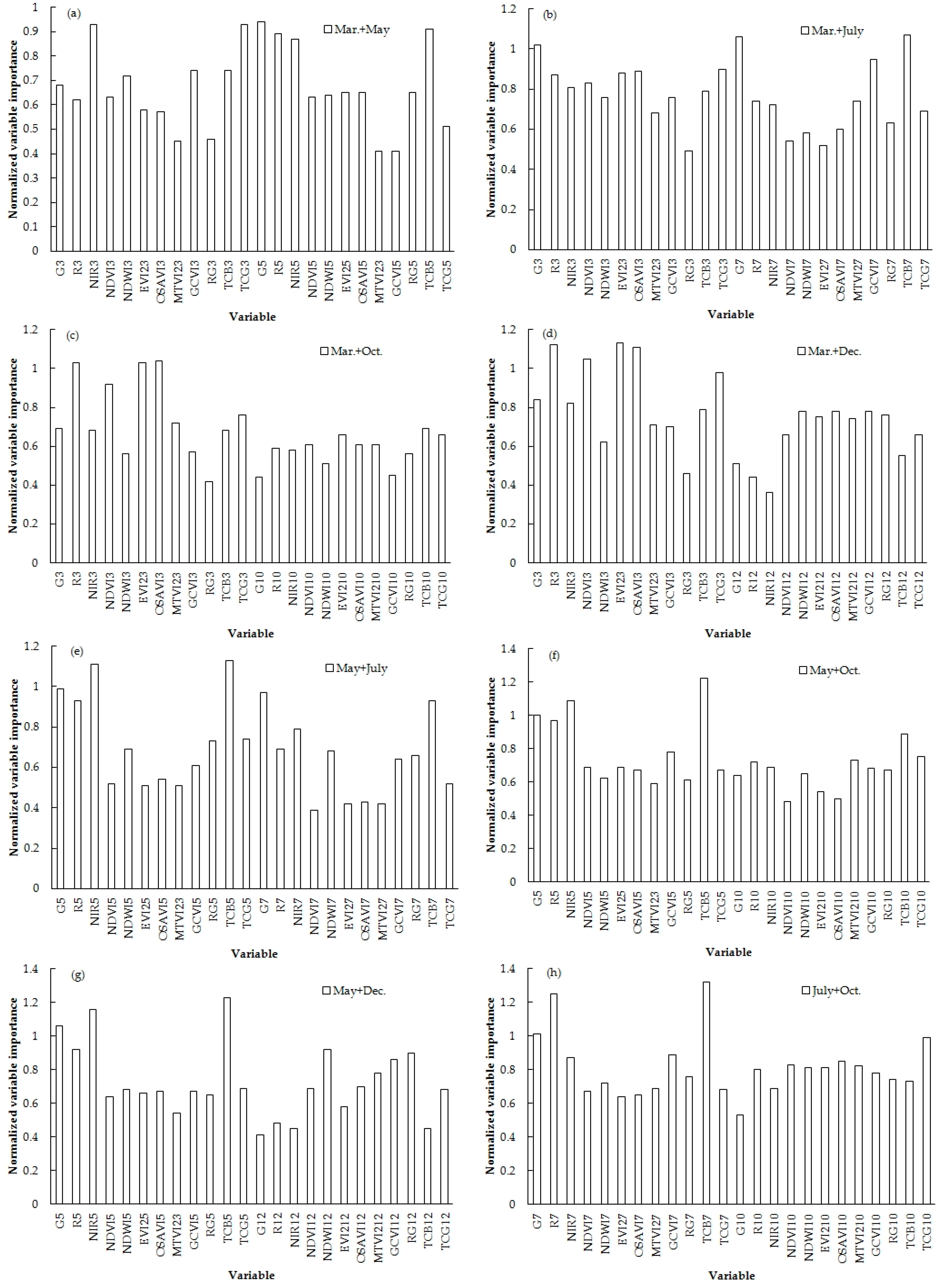
56,58,59]. In addition to the spectral bands, the spectral indices, temporal anomalies of spectral indices, biophysical variables, texture information, and topographic data were often stacked and used as input to the RF classifier. After random forest variable importance measures and the repeated classification accuracy assessment procedure were implemented, the optimal composition for input variables was determined as the input to the RF classifier to produce the final high classification result. Although temporal series approaches have received increasing attention, the multi-spectral and seasonal imagery-based classification for vegetation patches is still lacking.
The QVPs are visible with various composition components and spatial structures within the unused land of the YRD and were initially found through high spatial resolution SPOT 5 fusion-ready imagery in 2011 [71]. The QVPs appear to have a rapid succession rate and are ideal for studying the mechanism of spontaneous plant colonization and growth in this region, which will benefit the adaptive active restoration strategies implementation in the degraded wetland ecosystem of the YRD initiated in July 2002 [72]. Mapping QVPs is therefore important for a better understanding of vegetation patch patterns, formation and evolution mechanisms, and patch functioning. The single-date high-resolution imagery from different satellites such as SPOT 5, ALOS, ZY-3, QuickBird, China-Brazil Earth Resource Satellite (CBERS) 04, Gaofen (GF) 1 and GF-2 has been used to map the QVPs [16,28,29,30,71]. CBERS-04 imagery (with a spatial resolution of 5 m) is suitable for detecting the QVPs that are commonly found in an area of 25 km from the Bohai Sea of the YRD [16]. However, the classification accuracies for K-Means, DT, and SVM, are not stable, and are low in some cases [16,73]. Although comparison of the different seasonal CBERS-04 images for mapping QVPs has been carried out [73], the multi-spectral and seasonal imagery-based classification of QVPs remains unclear. For these reasons, the aim of this study was to explore the potential of multi-seasonal CBERS-04 images for mapping QVPs using the widely used RF classifier. CBERS-04 imagery acquired in the early spring, spring, summer, late autumn, and winter was used individually and the results were compared to provide insights into the optimal season for image acquisition. The different combinations of the different seasonal images were then used to evaluate the potential for using a multi-seasonal approach for mapping the QVPs.

2. Materials and Methods

2.1. Study Area

The study site is located 63 km northeast of Dongcheng District of Doongying City (118°7′ E–119°10′ E and 36°55′ N–38°10′ N) in Shandong Province, China (Figure 1a) and covers an area of 2.85 km2 (Figure 1b). This area is a low and flat unused land formed after the cofferdam of the Gudong Oil Field was built to prevent sea water erosion and facilitate oil exploration in 1988. The soil types in this area are Fluvisols and Solonchaks, and the soil textures vary from sandy loam to silty clay [74]. This area has a warm temperate continental monsoon climate, with distinct seasons, a mean annual evaporation of 1962 mm, and a mean annual rainfall of 580 mm; about 70% of the rain falls during the summer [74]. It has an aridity index (the ratio between mean annual rainfall and mean annual evaporation) taken by the United Nations Convention to Combat desertification (UNCCD) of 0.30, which belongs to semi-arid areas [75]. Suaeda salsa (the growing season from late April to middle November), Tamarix chinensis (the growing season from late March to early December), and Phragmites australis (the growing season from early April to middle November) are the three most common and widely distributed types of native plant species over the study area, and are also the main plant species in the QVPs (photo in Figure 1a). The landscape of this area is characterized by a two-phase mosaic composed of the QVPs interspersed in the bare soil matrix (Figure 1b). The formation mechanisms on the QVPs and pattern is under study now, the hypotheses of QVP occurrence attributed to the seismic exploration of Gudong Oil Field in the YRD still needs to be confirmed [76,77].
A total of 32 georeferenced data from three field surveys carried out in October 2013 [76], August 2017 [77], and May 2018 were used to identify the QVPs in the CBERS-04 imagery for inclusion in the reference dataset. The collection of georeferenced data were equally divided into a training dataset (the number of QVPs, bare soil, and bodies of water were 816 pixels, 1875 pixels, and 609 pixels, respectively) and an independent validation dataset (the number of the QVPs, bare soil, and the water area were 516 pixels, 536 pixels, and 358 pixels, respectively) for the RF classification and accuracy assessment.

2.2. CBERS-04 Data

The CBERS-04 satellite launched on 7 December 2014 has four sensors, one of which is a panchromatic and multispectral camera, characterized by a 5 m spatial resolution panchromatic band (band 1, 510–850 nm), three 10 m spatial resolution multispectral bands (band 2, 520–590 nm; band 3, 630–690 nm; band 4, 770–890 nm), and a swath width of 60 km [78]. Due to the limitation of cloud coverage and data acquisition, and considering image quality, only five CBERS-04 images acquired in 2015, 2016, and 2017 were used in the study, including an image from the early spring in March, one from the spring in May, one from the summer in July, one from the late autumn in October, and one from the winter in December (Table 1).
Twenty GCPs selected by the image-to-image approach (with a mean root mean square error of 0.35 pixels) were used to register the multispectral bands at 10 m × 10 m pixel size to the panchromatic bands at 5 m × 5 m pixel size using a quadratic polynomial near neighbor method in ENVI v5.1. Pan-sharpened 5 m multispectral images were then produced for the five acquisition dates using the Gram–Schmidt spectral sharpening technique, which is one of the usual image sharpening methods used for preserving the spectral information of images [38,73,79], embedded in ENVI v5.1. The quick atmospheric correction method embedded in ENVI v5.1 was used to convert the digital numbers of the CBERS-04 images to the spectral reflectance, which needs no extra aided data, and implements significantly faster than the physics-based approaches, generally creating spectral reflectance within approximately 15% of the most widely used physics-based approach, fast line-of-sight atmospheric analysis of spectral hypercubes [80]. To reduce data processing time, a subset of the CBERS-04 fusion imagery was clipped to focus on the study site (Figure 1b), which included QVPs, bare soil and bodies of water.
Due to the flat terrain and the difficulty in obtaining fine resolution digital elevation model data for the research area, topographic data were not used in this study. The variables from texture information were often low on the list of variable importance [33,34]. The spectral bands and the derived spectral indices were, therefore, most commonly applied [35,46,56]. In this study, three bands of pan-sharpened 5 m multispectral imagery, and nine spectral indices were used as predictive variables for the RF classification of the QVPs (Table 2), which can be derived from three multispectral bands (Near infrared (band 4), Red (band 3), and Green (band 2)) of CBERS-04, and have repeatedly been demonstrated to improve classification accuracy due to sensitivity to vegetation characteristics, insensitivity to soil effect, and the ability to capture both land surface features and the seasonal changes in the growth of vegetation [47,64,81,82,83,84]. Because there are no tasseled cap coefficients for spectral reflectance in the fusion CBERS-04 imagery for deriving the tasseled cap brightness (TCB) and greenness (TCG), the combined coefficients from five-date images used in this study were derived (Table 2) according to the Gram-Schmidt orthogonalization based method used in the previous study [85], and the TCB and TCG components were, thus, produced.

2.3. Random Forest Classification

As described in Section 1, the RF classifier was selected to classify the QVPs in this study. The RF classifier consists of an ensemble of multiple decision trees, each of which is built using a bootstrapped sample of the reference data and is assessed from the remaining sample of the reference data. The RF classifier has four main advantages, such as the small number of parameters that need to be adjusted, a low tendency to over-fit data, no data distribution assumptions that need to be met, and an ability to measure the importance of the input variables. The detailed introduction and theories on the RF classifier can be found in literature [94,95,96]. The RF classification was implemented using the ImageRF embedded in the EnMAP-Box v2.02, which is a freely available processing and analysis toolbox and can be integrated into the ENVI v5.1 classic menu to enhance the range of available applications [97]. The two main tuning parameters in RF, ntree (number of trees to be grown, the default value in ntree = 500) and mtry (number of possible splitting variables to be considered at each tree node, the default value of mtry = the number of the square root of the total predictive variables), were set to their default values because previous studies have demonstrated that the default values are generally a good choice [34,35,98].
The use of combined multi-season images for detecting QVPs has been lacking, and the potential of multi-seasonal CBERS-04 images remain unclear. It is necessary to compare the differences between the data acquisition periods and to find optimal composition periods, classifications were carried out on the CBERS-04 data separately from the five different dates and the twenty-six combined datasets (all possible combinations of the five images were the ten two-season combined images, the ten three-season combined images, the five four-season combined images, and the one five-season combined image) in a multi-date approach. A backward variable removing procedure was used to select the optimal feature datasets for every dataset for building a RF model through an assessment of variable importance produced by the RF model based on mean decrease in classification accuracy and the minimum mean square error calculated from the out-of–bag data and RF model classification accuracy. On the basis of ranking the importance of predictive variables, firstly, the least important predictive variable was removed, and the remaining variables were used to reclassify, then, the second least important predictive variable was removed, and the remaining variables were used to reclassify. This process was repeated until only the three most important predictive variables for single season image (the predictive variables at least containing one variable of every image for multi-season combined images) were left and the classification was stopped. Finally, the variables that can obtain the highest classification accuracy were selected as the predictive variables for the final RF classification model. During the process of classification and accuracy assessment, the same training and validation dataset was used to avoid differences induced by the reference dataset variability. Accuracy assessment of the classification results was presented in a confusion matrix and measured according to the producer’s (PA) and user’s accuracy (UA), overall accuracy (OA), and the Kappa coefficient.
Next a successive identification was performed, where a majority analysis with a 3 × 3 kernel size was first used to match the salt and pepper noise pixels within a large single class with a large single class, followed by a change in the classification to vector analysis in order to separate the QVPs from the non-QVP vegetation based on the thresholds of area (less than 3000 m2) and perimeter/area (less than 0.54), as determined by previous results [16,28,73]. The precision rate (Ad), recall rate (Ar), and F measure (F) were then used to analyze the final detection accuracy of the QVPs; these factors have often been used for performance measures in pattern recognition, information retrieval, machine learning and binary classification [73,99].

3. Results

3.1. Single Season Image

3.1.1. Predictive Variable Importance

The effects of the different predictive variables on the land cover classification results from five single season data are listed in Figure 2. The importance of the predictive variables diverges considerably between the seasons of image acquisition. The best important variable for the classification success was the green band (G) for the early spring month of March, the TCG for the spring and summer months of May–July, and the MTVI2 for the late autumn and winter months of October–December. This reflects the seasonal characteristics of the two-phase mosaic of the study area and the best spectral indices for monitoring them. This may be explained by the fact that in early spring the vegetation begins to grow, and the original spectral bands can reflect the landscape features well. In spring and summer, the vegetation becomes green and dense, and the TCG can better monitor QVPs and bare soils. In late autumn and winter, the vegetation becomes yellow and sparse, and the MTVI2 is sensitive to high leaf area index and relatively insensitive to leaf chlorophyll content and soil effect [81,89], and therefore, can effectively monitor landscape features.

3.1.2. Predictive Variable Selection

The outcome of the predictive variable selection is listed in Table 3. Several of the predictive variables were identified as redundant in each of the datasets, and were therefore, removed from the final RF classification model. The number of predictive variables included in the final RF classification models was similar between the five datasets. Another observation was that the green band (G) was included in all of the five final RF classification models. The NDVI, NDWI, EVI2, OSAVI, MTVI2 and GCVI vegetation indices appeared to contribute relatively little to the classification success for all of five datasets. For the late autumn October and the winter December datasets, the three original spectral bands (red, near-infrared, and green bands) were slightly better for RF classification (for the October image, OA = 92.8%, Kappa = 0.890; for the December image, OA = 93.9%, Kappa = 0.906) than all twelve predictive variables and the minimum predictive variable datasets derived from all twelve predictive variables (for the October image, OA = 91.3%, Kappa = 0.867; for the December image, OA = 93.7%, Kappa = 0.903). Therefore, only the three original spectral bands were used in the final RF classification model for the October and December image.

3.1.3. The QVP Classification Results

The overall classification accuracies and Kappa coefficients resulting from the use of the five predictive variable datasets are presented in Figure 3. The results show that land cover classification based on the early spring data acquired on 27 March 2017 (OA = 98.1%, Kappa = 0.971) was more accurate than the classification based on the other four seasonal data. The lowest classification accuracy was obtained from the late autumn data, acquired on 24 October 2015 image (OA = 92.8%, Kappa = 0.890). Due to limited space, only the confusion matrix of the 27 March 2017 is presented in Table 4. The error of commission and omission was mainly because of the confusion between the QVPs and the bare soil, and the error of commission and omission between the QVPs and bodies of water were only found in the May and July images. This may be attributed to growth of aquatic plants during these periods. The error of commission and omission between the bare soil and the bodies of water existed only in the December image.
Through the visual interpretation of the Quickbird image (with a spatial resolution of 0.6 m) carried out with ENVI 5.1 software with the multi-temporal finer spatial resolution images from Google Earth and the multi-temporal CBERS-04 images, we identified 139 QVPs distributed in the study area [16,73], which was used as the correct number of QVPs to calculate the precision rate, recall rate, and F measure for assessing the final detection accuracy of the QVPs. The precision rate, recall rate, and F measure resulting from the use of the five predictive variable datasets are presented in Figure 4, which displays a similar curve to the overall classification accuracies and Kappa coefficients for land cover classification presented in Figure 3. The results show that the QVP detection based on the early spring data acquired on 27 March 2017 (Ad = 56.1%, Ar = 43.2%, F = 0.488) was more accurate than the classification based on the other four seasonal datasets. The lowest detection accuracy was obtained from the late autumn data acquired on the image from the 24 October 2015 (Ad = 40.7%, Ar = 25.2%, F = 0.311).

3.2. Two-Season Combined Images

3.2.1. Predictive Variable Importance and Selection

There were ten combined datasets in a two-season approach. The influence of the different predictive variables on land cover classification results from the ten combined datasets and the outcome of the predictive variable selection are shown in Figure 5 and Table 5. The number of predictive variables included in the final classification models differs considerably between the ten datasets (Table 5). The four datasets, including the March image, showed that the importance of the predictive variables for March was similar to that for May, and was relatively higher than for the July, October, and December images. From the three datasets, including the May image, it appeared that the importance of the predictive variables for May was relatively higher than those for the July, October, and December images. The number of predictive variables for the October and December images, including in the final classification models of the two datasets with the July image, exceeded that associated with the July image. For the October–December combined dataset, the number of predictive variables for the October image exceeded that of the December image. These results demonstrate the different effects that the different seasonal images have on the classification success.

3.2.2. The QVP Classification Results

The overall classification accuracies and Kappa coefficients resulting from the use of the ten predictive variable datasets are presented in Figure 6. The results show that land cover classification based on the combined March–October dataset (OA = 99.4%, Kappa = 0.990) was more accurate than the classification based on the other nine combined two-season datasets. The lowest classification accuracy was obtained from the combined May–December dataset (OA = 96.8%, Kappa = 0.951). Due to limited space, only the confusion matrix of the combined March–October dataset is presented in Table 6. The error of commission and omission was mainly from the confusion between the QVPs and bare soils.
The precision rate, recall rate, and F measure resulting from the ten combined two-season datasets are presented in Figure 7. The highest precision rate, recall rate, and F measure were from the combined March–December image (Ad = 66.3%), the combined March–July image (Ar = 47.5%), and the combined March–December image (F = 0.528), respectively. The lowest precision rate, recall rate, and F measure were from the combined May–December image (Ad = 37.2%), the combined October–December image (Ar = 23.7%), and the combined October–December image (F = 0.313), respectively. The results show that the detection of QVPs based on the combined March–December image (Ad = 66.3%, Ar = 43.9%, F = 0.528) was more accurate than the classification based on the other nine two-season datasets.

3.3. Three-Season Combined Images

There were ten combined datasets in the three-season approach. The number of predictive variables included in the final RF classification models was 34 for March–May–July, 17 for March–May–October, 35 for March–May–December, 24 for March–July–October, 27 for March–July–December, 25 for March–October–December, 27 for May–July–October, 17 for May–July–December, 35 for May–October–December, and 31 for July–October–December combined datasets, respectively. The overall classification accuracies and Kappa coefficients resulting from the use of the ten predictive variable datasets are presented in Figure 8. The results show that land cover classification based on the combined March–July–December dataset (OA = 99.8%, Kappa = 0.997) was more accurate than the classification based on the other nine combined two-season datasets. The lowest classification accuracy was obtained from the combined March–May–December dataset (OA = 97.0%, Kappa = 0.954). Due to limited space, only the confusion matrix for the combined March–July–December dataset is presented in Table 7. The error of commission and omission was mainly from the confusion between the QVPs and bare soils.
The precision rate, recall rate, and F measure resulting from the ten combined three-season datasets are presented in Figure 9. The results show that the detection of QVPs based on the combined March–October–December dataset (Ad = 64.0%, Ar = 41.0%, F = 0.500) was more accurate than the classification based on the other nine three-season datasets. The lowest detection accuracy was obtained from the combined Match–May–October dataset (Ad = 37.5%, Ar = 28.1%, F = 0.321).

3.4. Four-Season Combined Images

There were five combined datasets for the four-season approach. The number of predictive variables included in the final RF classification models was 46 for March–May–July–October, 21 for March–May–July–December, 27 for March–May–October–December, 26 for March–July–October–December, and 42 for May–July–October–December, respectively.
The overall classification accuracies and Kappa coefficients resulting from the use of the five predictive variable datasets are presented in Figure 10. The results show that land cover classification based on the combined March–July–October–December dataset (OA = 99.8%, Kappa = 0.997) was more accurate than the classification based on the other four combined two-season datasets. The lowest classification accuracy was obtained from the combined March–May–October–December dataset (OA = 97.8%, Kappa = 0.967). The confusion matrix, Producer’s and User’s accuracies of the three land cover classes from the combined March–July–October–December dataset were similar to those of the combined March–July–December dataset displayed in Table 7. The error of commission and omission was mainly from the confusion between the QVPs and bare soils.
The precision rate, recall rate, and F measure resulting from the five combined four-season datasets are presented in Figure 11. The results show that the QVP detection based on the combined March–July–October–December dataset (Ad = 60.2%, Ar = 40.3%, F = 0.483) was more accurate than the classification based on the other four four-season datasets. The lowest precision rate, recall rate, and F measure were from the combined May–July–October–December dataset (Ad = 38.2%), the combined March–May–July–October dataset (Ar = 26.6%), and the combined March–May–July–October dataset (F = 0.316), respectively.

3.5. Five-Season Combined Image

The number of predictive variables included in the final RF classification models was fifty-eight for the combined five-season dataset. The land cover classification accuracy was OA = 98.7%, Kappa = 0.978. The confusion matrix for the combined March–May–July–October–December dataset is presented in Table 8. The error of commission and omission was mainly from the confusion between the QVPs and bare soils. The precision rate, recall rate, and F measure resulting from the combined five-season dataset were Ad = 37.3%, Ar = 27.3%, and F = 0.315, respectively.

3.6. Comparisons

Table 9 shows the comparison analyses of the optimal classification results for the five different combinations in the number of seasons using the overall accuracy (OA), Kappa coefficient (Kappa), precision rate, recall rate, and F measure values. The comparison in the results indicates that the influence from the March image is significant. The OA and Kappa values increased slightly from the optimal individual seasonal imagery to season combined image datasets, and the precision rate, recall rate, and F measure values increased moderately, except for those associated with the combined five-season dataset. Finally, the results suggest that the March–December combination dataset was the optimal choice for the detection of QVPs (Figure 12).

4. Discussion

Previous research results for the YRD had demonstrated that different seasonal QVP classification from CBERS-04 imagery had variable accuracy, and that the spring imagery could detect the QVPs more precisely and completely when compared with the other seasonal images [73], but the use of combined multi-season images for detecting QVPs has been lacking. In fact, the use of multi-seasonal images has been demonstrated as statistically important for the mapping of tree species [35,37,38]. The importance of this study was in demonstrating that the seasonal influence in multi-season CBERS-04 images for classifying land cover and detecting QVPs was significant. This study showed that accurate land cover classification can be achieved for the distribution of QVPs in the YRD by applying both single season and multi-seasonal fusion CBERS-04 high spatial resolution (5 m) multispectral images (best result OA = 99.8%, Kappa = 0.997). Errors in the classification mainly existed between the QVPs and the bare soil. However, as in previous studies [16,
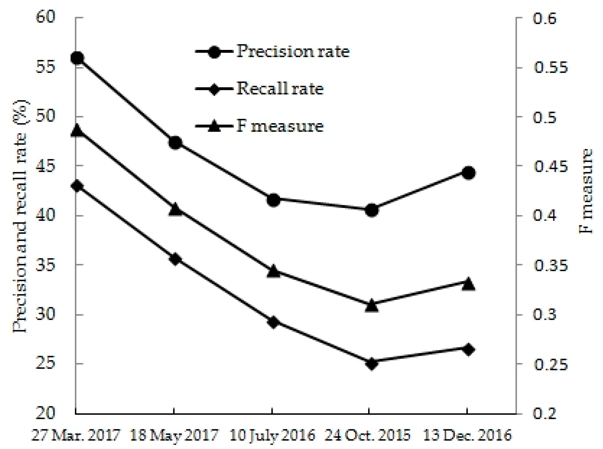
73], the detection accuracy of the QVPs was low (best result precision rate = 66.3%, recall rate = 47.5%, F measure = 0.528). This low detection accuracy may be attributed to the omission of the smaller size QVPs (less than 3 × 3 pixels), or the coalescence between the QVPs with other QVPs or other vegetation.
Our comparison analysis demonstrates that both the March image and multi-seasonal fusion CBERS-04 high spatial resolution multispectral images including the March image, can produce high overall classification accuracies for land cover, and the multi-season combined images only increased 0.6–1.7% in overall accuracy as compared to the use of the March image alone. The research result of this study indicated that March and May were more suitable acquisition periods for single date imagery used for land cover mapping and QVP detection in this study area, which was consistent with that of Liu [73]. The reason for the higher accuracies of the spring season classification over the summer season (the peak of growing season of vegetation with the greatest difference between vegetation and bare soil) are unpredictable, but some key observations during the field investigation can be used to explain this phenomenon. (1) Bare soil becomes brighter because of desiccation and soil salt accumulation in the spring, which increases the contrast between QVPs and bare soil, whereas the summer rainfall results in increases in soil moisture, therefore decreasing the contrast between the QVPs and the bare soil. (2) The gap between the QVPs and other strips of vegetation can be blurred due to the coalescence between vegetation elements in either summer or autumn season [73]. For single season imagery, the October (autumn season, the end of growing season of vegetation) produced the lowest overall classification accuracy for land cover, which through visual inspections and comparisons on five images (Figure 13) could be attributed to the small difference between the vegetation and bare soil area and more coalescence between vegetation elements. The highest classification accuracies for land cover from two-season, three-season, and four-season combined datasets were obtained from the May–October (OA = 99.4%), March–July–December (OA = 99.8%), and the March–July–October–December (OA = 99.8%) combined images respectively. The lowest classification accuracies for land cover from two-season, three-season, and four-season combined datasets were obtained from the MayvDecember (OA = 96.8%), March–May–December (OA = 97.0%), and the March–May–October–December (OA = 97.8%) combined images, respectively. These results indicated that adding imagery into classification could help to improve the accuracies for mapping land cover, which is consistent with the previous researches [45,46,55,58], but the increase in accuracy was limited. The March–May–October–December combined data had the lowest classification accuracy of all four-season combined datasets, which indicated that the combined data consisting of images with less contrasts or similar phenological features had the low capability for mapping land cover. It also showed that the combination of different season images with the higher classification accuracy for land cover was not necessarily an optimal combination of multi-season images, whereas the combination of the different season images with the different landscape temporal features, especially the phenological features of vegetation may be an optimal combination of multi-season images, and could further improve the classification accuracy for mapping land cover and detecting the QVPs.
Through one-sample t test analysis on Kappa values in SPSS 19.0 software (SPSS, Chicago, IL., USA), it indicated that the land cover classification results were statistically significant different for among single season images (p = 0.041), among two-season combined data (p = 0.002), and among three-season combined data (p = 0.025), and those from four-season combined data were not statistically significant different (p = 0.243). The independent-samples T test detected statistically significant differences of Kappa values between the single season and two-season (p = 0.039), the single season and three-season (p = 0.025), and the single season and four-season (p = 0.018) combined data, and no significant differences of Kappa values between the other combined data.
In general, the optimal seasonal combination data which had a high accuracy for classifying land cover could produce a high accuracy for detecting the QVPs (shown in Figure 3, Figure 4, Figure 10 and Figure 11). However, for the two-season and three-season combination datasets, the optimal seasonal combination data which had a high accuracy for classifying land cover did not necessarily produce a high accuracy for detecting the QVPs (Figure 6, Figure 7, Figure 8 and Figure 9). The main possible reason may be due to the coalescence between the QVPs and other vegetation elements which made the thresholds of area and shape less effective for detecting the QVPs from land cover map. The March–December spring-winter season combined images had the best result for detecting the QVPs compared to the single season and other multi-season combined images. Except the high difference between the QVPs and bare soil in the two images, one possible reason may be that Tamarix chinensis, one of the main plant species composed of the QVPs, is easier to be identified in late fall and early winter [100]. This is not consistent with the higher classification results for tree species mapping by applying the dry-wet season combined images [35,37,38], which may be due to the different geographical and phenological characteristics, and soil salinization. In general, increasing temporal imagery acquisition frequencies can help to improve the classification accuracies [46,55,58]. However, there still is an optimization of image acquisition timing and frequency for different research objects with different resolution imagery in different regions [58,66]. Our assessment results indicated that the March–December spring-winter season combined images produces optimal multi-season combined data when the multi-season images are to be used for detection of QVPs, and that the combined images including those of more than two seasons could not effectively improve the classification accuracy, which is in line with the conclusion that adding more images could not increase the value for classifying tree species [36]. This finding must be interpreted with caution because there were only five images used in this study.
Figure 14 shows the thirty-one pairs of comparison analyses of the optimal classification results for mapping land covers with and without nine spectral indices using the overall accuracy (OA) and Kappa coefficient (Kappa). The optimal classification results for mapping land covers including nine spectral indices had higher OA and Kappa values than those without nine spectral indices, except for the October and December images. However, the difference of 0–2.3% for OA and 0–0.035 for Kappa was small between the thirty-one pairs with and without those indices, and twenty-eight of the thirty-one pairs had less than 1% OA difference and less than 0.02 Kappa difference. The paired-sample t test detected no statistically significant differences of Kappa values between the land cover classification results from the combined data with and without nine spectral indices (p = 0.003). This result indicated that the nine spectral indices derived from the three original spectral bands contributed low value for land cover classification. It must be especially considered that when a classification is to be carried out over a large study area, larger data storage and longer processing times are required.
Although the optimal seasonal CBERS-04 images along with effective predictive variable datasets were used, the low detection accuracies presented in this study are similar to previous research results where the individual seasonal high spatial resolution data, including those from CBERS-04, have been used for detecting QVPs using the OBIA classification with K-Means, KNN and SVM classifiers [16,73]. This indicated that the choice of the classifier itself could not greatly improve the classification accuracy of the QVPs, which is in line with the opinion that the selection of the classifier itself was of low significance if the data is adequate in meeting the demands of the classifier [36].
It is possible to improve QVP mapping through three approaches in the future. (1) Additional texture features are included in the RF classification for the QVPs. Texture features have been proved important in the mapping of invasive Fallopia japonica [32], larch plantations [33], urban tree species [34] and plastic-mulched farmland [101]. (2) The sub-meter level resolution data are applied. When the gaps between QVPs or between QVPs and other strips of vegetation are less than 5 m, or the diameter of a QVP is less than 10 m, the 5 m spatial resolution of CBERS-04 imagery is not enough to detect the QVPs. Therefore, it is necessary to further improve spatial resolution [16,38]. (3) Higher spectral resolution data are applied. The WorldView-2 imagery has higher spectral resolution and unique spectral bands such the red edge band, shortwave bands, and has therefore demonstrated higher accuracy for the classification of tree species than other images with a similar or higher spatial resolution [35,38]. This is therefore a good choice for detecting QVPs in the YRD in the future.

5. Conclusions

This study has investigated the potential of multi-season CBERS-04 imagery for mapping the QVPs commonly found in the YRD, which extends from the Liaohe Delta to the coastal salt marshes in Northern Jiangsu Province, China. Classification was performed using the RF classification approach. Thirty-one different datasets including three spectral bands and nine spectral indices derived from the five fusion 5 m CBERS-04 multispectral images were compared for their capabilities of classifying land covers and detecting QVPs to evaluate the seasonal influences on classification accuracy. The main conclusions resulting from this research are as follows:
The early spring season image (March) produced a higher classification accuracy compared to all other individual season CBERS-04 images.
All of the optimal classifications resulted from the different combinations that include the early spring season image, which indicated that the early spring season image contributed much to classification success.
A typical early spring-winter (December and March) combined CBERS-04 images performed better for mapping the QVPs than the other multi-season combined image datasets.
The five-season combination images (March, May, July, October, and December) had the lowest classification accuracy for mapping QVPs.
Although the optimal classification results including nine spectral indices had higher OA and Kappa values than those without those indices, the improvement in overall accuracy was small. Therefore, the gain in accuracy should be balanced against the increase in processing time and storage space when using the derived spectral indices.
The choice of the classifier itself could not greatly improve classification accuracy from the CBERS-04 imagery. Improved classification accuracy will most likely be achieved through use of the higher spatial and spectral resolution data such as GF-2, WorldView-2, and WordView-3. The improvement in spectral resolution is more important for mapping QVPs than the improvement in spatial resolution.
Our work shows that it is important to choose suitable seasonal imagery for mapping of QVPs. The research results from this study also indicated that there is an optimization of image acquisition timing and frequency, and that adding more seasonal data for mapping the QVPs may not be worth the gain in classification accuracy, and may even reduce the classification accuracy. Future research should focus on (1) comparison analysis based on more seasonal data and more areas, (2) applying higher spatial and spectral resolution imagery to map the QVPs, and (3) map the components and structure of the QVPs, which is important for studying the evolution models of the QVPs.

Author Contributions

Conceptualization, Q.L. and G.L.; methodology and data analysis, Q.L., H.S., and H.L.; validation, C.H.; writing—original draft preparation, Q.L.; writing—review and editing, Q.L., H.S., G.L., C.H. and H.L.; funding acquisition, G.L. and Q.L.

Funding

This research was jointly financially supported by the National Natural Science Foundation of China (Project Nos. 41671422, 41661144030, 4151144012), the Strategic Priority Research Program of Chinese Academy of Sciences (Project No. XDA20030302), the Innovation Project of LREIS (Project Nos. O88RA20CYA, 08R8A010YA), and the National Mountain Flood Disaster Investigation Project (SHZH-IWHR-57).

Acknowledgments

Thanks to China Center of Resources Satellite Data and Application for providing the CBERS-04 data products.

Conflicts of Interest

The authors declare no conflict of interest.

References

  1. Aguiar, M.R.; Sala, O.E. Patch structure, dynamics and implication for the functioning of arid ecosystem. Tree 1999, 14, 273–277. [Google Scholar] [CrossRef]
  2. Couteron, P.; Lejeune, O. Periodic spotted patterns in semi-arid vegetation explained by a propagation-inhibition model. J. Ecol. 2001, 89, 616–628. [Google Scholar] [CrossRef]
  3. Valentin, C.; d’Herbes, J.M.; Poesen, J. Soil and water components of banded vegetation patterns. Catena 1999, 37, 1–24. [Google Scholar] [CrossRef]
  4. Shoshany, M.; Kelman, E. Assessing mutuality of change in soil and vegetation patch pattern characteristics by means of cellular automata simulation. Geomorphology 2006, 77, 35–46. [Google Scholar] [CrossRef]
  5. Janeau, J.L.; Mauchamp, A.; Tarin, G. The soil surface characteristics of vegetation stripes in Northern Mexico and their influences on the system hydrodynamics: An experimental approach. Catena 1999, 37, 165–173. [Google Scholar] [CrossRef]
  6. Galle, S.; Ehrmann, M.; Peugeot, C. Water balance in a banded vegetation pattern: A case study of tiger bush in western Niger. Catena 1999, 37, 165–173. [Google Scholar] [CrossRef]
  7. Dunkerley, D.L.; Brown, K.J. Oblique vegetation banding in the Australian arid zone: Implications for theories of pattern evolution and maintenance. J. Arid Environ. 2002, 51, 163–181. [Google Scholar] [CrossRef]
  8. Saco, P.M.; Willgoose, G.R.; Hancock, G.R. Eco-geomorphology of banded vegetation patterns in arid and semi-arid regions. Hydrol. Earth Syst. Sci. 2007, 11, 1717–1730. [Google Scholar] [CrossRef] [Green Version]
  9. Frenkel, R.E.; Boss, T.R. Introduction, establishment and spread of Spartina patens on Cox Island, Siuslaw Estuary, Oregon. Wetlands 1988, 8, 33–49. [Google Scholar] [CrossRef]
  10. Webster, R.; Maestre, E.T. Spatial analysis of semi-arid patchy vegetation by the cumulative distribution of patch boundary spacings and transition probabilities. Environ. Ecol. Stat. 2004, 11, 257–281. [Google Scholar] [CrossRef]
  11. Armas, C.; Pugnaire, F.I.; Sala, O.E. Patch structure dynamics and mechanisms of cyclical succession in a Patagonian steppe (Argentina). J. Arid Environ. 2008, 72, 1552–1561. [Google Scholar] [CrossRef]
  12. Sheffer, E.; Yizhaq, H.; Shachak, M.; Meron, E. Mechanism of vegetation-ring formation in water-limited systems. J. Theor. Biol. 2011, 273, 138–146. [Google Scholar] [CrossRef]
  13. Tschinkel, W.R. The life cycle and life span of Namibian fairy circles. PLoS ONE 2012, 7, e38056. [Google Scholar] [CrossRef]
  14. Bordeu, I.; Clerc, M.G.; Couterons, P.; Lefever, R.; Tlidi, M. Self-replication of localized vegetation patches in scarce environments. Sci. Rep. 2016, 6, 33703. [Google Scholar] [CrossRef]
  15. Mora, J.L.; Lazaro, R. Evidence of a threshold in soil erodibility generating differences in vegetation development and resilience between two semiarid grasslands. J. Arid Environ. 2013, 89, 57–66. [Google Scholar] [CrossRef]
  16. Liu, Q.S.; Huang, C.; Liu, G.H.; Yu, B.W. Comparison of CBERS-04, GF-1, and GF-2 satellite panchromatic images for mapping quasi-circular vegetation patches in the Yellow River Delta, China. Sensors 2018, 18, 2733. [Google Scholar] [CrossRef]
  17. Rietkerk, M.; Dekker, S.C.; De Ruiter, P.C.; Van de Koppel, J. Self-organized patchiness and catastrophic shifts in ecosystems. Science 2004, 305, 1926–1929. [Google Scholar] [CrossRef]
  18. Von Hardenberg, J.; Kletter, A.Y.; Yizhaq, H.; Nathan, J.; Meron, E. Periodic versus scale-free patterns in dryland vegetation. Proc. R. Soc. B 2010, 277, 1771–1776. [Google Scholar] [CrossRef] [Green Version]
  19. Kakembo, V. Vegetation patchiness and implications for landscape function: The case of Pteronia incana invader species in Ngqushwa Rural Municipality, Eastern Cape, South Africa. Catena 2009, 77, 180–186. [Google Scholar] [CrossRef]
  20. Kadmon, R.; Harari-Kremer, R. Studying long-term vegetation dynamics using digital processing of historical aerial photographs. Remote Sens. Environ. 1999, 68, 164–176. [Google Scholar] [CrossRef]
  21. Becker, T.; Getzin, S. The fairy circles of Kaokoland (North-West Namibia) origin, distribution, and characteristics. Basic Appl. Ecol. 2000, 1, 149–159. [Google Scholar] [CrossRef] [Green Version]
  22. Strand, E.K.; Smith, A.M.S.; Bunting, S.C.; Vierling, L.A.; Hann, D.B.; Gessler, P.E. Wavelet estimation of plant spatial patterns in multitemporal aerial photography. Int. J. Remote Sens. 2006, 27, 2049–2054. [Google Scholar] [CrossRef]
  23. Odindi, J.O.; Kakembo, V. Comparison of pixel and sub-pixel based techniques to separate Pteronia incana invaded areas using multi-temporal high-resolution imagery. J. Appl. Remote Sens. 2009, 3, 033545. [Google Scholar] [CrossRef]
  24. Barbier, N.; Couteron, P.; Lejoly, J.; Deblauwe, V.; Lejeune, O. Self-organized vegetation patterning as a fingerprint of climate and human impact on semi-arid ecosystems. J. Ecol. 2006, 94, 537–547. [Google Scholar] [CrossRef]
  25. Shekede, M.D.; Murwira, A.; Masocha, M. Wavelet-based detection of bush encroachment in a savanna using multi-temporal aerial photographs and satellite imagery. Int. J. Appl. Earth Obs. Geoinf. 2015, 35, 209–2016. [Google Scholar] [CrossRef]
  26. Laliberte, A.S.; Rango, A.; Havstad, K.M.; Paris, J.F.; Beck, R.F.; McNeely, R.; Gonzalez, A.L. Object-oriented image analysis for mapping shrub encroachment from 1937 to 2003 in southern New Mexico. Remote Sens. Environ. 2004, 93, 198–210. [Google Scholar] [CrossRef]
  27. Boggs, G.S. Assessment of SPOT 5 and QuickBird remotely sensed imagery for mapping tree cover in savannas. Int. J. Appl. Earth Obs. 2010, 12, 217–224. [Google Scholar] [CrossRef]
  28. Liu, Q.S.; Liu, G.H.; Huang, C.; Xie, C.J. Using SPOT 5 fusion-ready imagery to detect Chinese tamarisk (saltcedar) with mathematical morphological method. Int. J. Digit. Earth 2014, 7, 217–228. [Google Scholar] [CrossRef]
  29. Liu, Q.S.; Liu, G.H.; Huang, C.; Xie, C.J.; Shi, L. Using ALOS high spatial resolution image to detect vegetation patches. Procedia Environ. Sci. 2011, 10, 896–901. [Google Scholar] [CrossRef]
  30. Liu, Q.S.; Zhang, Y.J.; Liu, G.H.; Huang, C. Detection of quasi-circular vegetation community patches using circular hough transform based on ZY-3 satellite image in the Yellow River Delta, China. In Proceedings of the International Geoscience and Remote Sensing Symposium, Melbourne, Australia, 21–26 July 2013; IEEE: New York, NY, USA, 2013; pp. 2149–2151. [Google Scholar]
  31. Fernandes, M.R.; Aguiar, F.C.; Silva, J.M.N.; Ferreira, M.T.; Pereira, J.M.C. Optimal attributes for the object based detection of giant reed in riparian habitats: A comparative study between Airborne High Spatial Resolution and WorldView-2 imagery. Int. J. Appl. Earth Obs. 2014, 32, 79–91. [Google Scholar] [CrossRef]
  32. Dorigo, W.; Lucieer, A.; Podobnikar, T.; Carni, A. Mapping invasive Fallopia japonica by combined spectral, spatial, and temporal analysis of digital orthophotos. Int. J. Appl. Earth Obs. 2012, 19, 185–195. [Google Scholar] [CrossRef]
  33. Gao, T.; Zhu, J.J.; Zheng, X.; Shang, G.D.; Huang, L.Y.; Wu, S.R. Mapping spatial distribution of larch plantations from multi-Seasonal Landsat-8 OLI imagery and multi-scale textures using random forests. Remote Sens. 2015, 7, 1702–1720. [Google Scholar] [CrossRef]
  34. Li, D.; Ke, Y.H.; Gong, H.L.; Li, X.J. Object-based urban tree species classification using bi-temporal WorldView-2 and WorldView-3 images. Remote Sens. 2015, 7, 16917–16937. [Google Scholar] [CrossRef]
  35. Karlson, M.; Ostwald, M.; Reese, H.; Bazie, H.R.; Tankoana, B. Assessing the potential of multi-seasonal WorldView-2 imagery for mapping West African agroforestry tree species. Int. J. Appl. Earth Obs. 2016, 50, 80–88. [Google Scholar] [CrossRef]
  36. Fassnacht, F.E.; Latifi, H.; Sterenczak, K.; Modzelewska, A.; Lefsky, M.; Waser, L.T.; Straub, C.; Ghosh, A. Review of studies on tree species classification from remotely sensed data. Remote Sens. Environ. 2016, 186, 64–87. [Google Scholar] [CrossRef]
  37. Madonsela, S.; Cho, M.Z.; Mathieu, R.; Mutanga, O.; Ramoelo, A.; Kaszta, Z.; Kerchove, R.V.D.; Wolff, E. Multi-phenology WorldView-2 imagery improves remote sensing of savannah tree species. Int. J. Appl. Earth Obs. 2017, 58, 65–73. [Google Scholar] [CrossRef] [Green Version]
  38. Pu, R.L.; Landry, S.; Yu, Q.Y. Assessing the potential of multi-seasonal high-resolution Pleiades satellite imagery for mapping urban tree species. Int. J. Appl. Earth Obs. 2018, 71, 144–158. [Google Scholar] [CrossRef]
  39. Wu, J.W.; Yao, W.; Polewski, P. Mapping Individual Tree Species and Vitality along Urban Road Corridors with LiDAR and Imaging Sensors: Point Density versus View Perspective. Remote Sens. 2018, 10, 1403. [Google Scholar] [CrossRef]
  40. Gudex-Cross, D.; Pontius, J.; Adams, A. Enhanced forest cover mapping using spectral unmixing and object-based classification of multi-temporal Landsat imagery. Remote Sens. Environ. 2017, 196, 193–204. [Google Scholar] [CrossRef]
  41. Clark, M.L.; Buck-Diaz, J.; Evens, J. Mapping of forest alliances with simulated multi-seasonal hyperspectral satellite imagery. Remote Sens. Environ. 2018, 210, 490–507. [Google Scholar] [CrossRef]
  42. Higginbottom, T.P.; Symeonakis, E.; Meyer, H.; Linden, S.V.D. Mapping fractional woody cover in semi-arid savannahs using multi-seasonal composites from Landsat data. ISPRS J. Photogramm. Remote Sens. 2018, 139, 88–102. [Google Scholar] [CrossRef] [Green Version]
  43. Low, F.; Knofel, P.; Conrad, C. Analysis of uncertainty in multi-temporal object-based classification. ISPRS J. Photogramm. Remote Sens. 2015, 105, 91–106. [Google Scholar] [CrossRef]
  44. Hutt, C.; Koppe, W.; Miao, Y.X.; Bareth, G. Best accuracy land use/land cover (LULC) classification to derive crop types using multitemporal, multisensor, and multi-polarization SAR satellite images. Remote Sens. 2016, 8, 684. [Google Scholar] [CrossRef]
  45. Veloso, A.; Mermoz, S.; Bouvet, A.; Toan, T.L.; Planells, M.; Dejoux, J.; Ceschina, E. Understanding the temporal behavior of crops using Sentinel-1 and Sentinel-2-like data for agricultural applications. Remote Sens. Environ. 2017, 199, 415–426. [Google Scholar] [CrossRef]
  46. Vuolo, F.; Neuwirth, M.; Immitzer, M.; Atzberger, C.; Ng, W.T. How much does multi-temporal Sentinel-2 data improve crop type classification? Int. J. Appl. Earth Obs. 2018, 72, 122–130. [Google Scholar] [CrossRef]
  47. Cai, Y.P.; Guan, K.Y.; Peng, J.; Wang, S.W.; Seifert, C.; Wardlow, B.; Li, Z. A high-performance and in-season classification system of field-level crop types using time-series Landsat data and a machine learning approach. Remote Sens. Environ. 2018, 210, 35–47. [Google Scholar] [CrossRef]
  48. Hao, P.Y.; Wu, M.Q.; Niu, Z.; Wang, L.; Zhan, Y.L. Estimation of different data compositions for early-season crop type classification. PeerJ 2018, 6, e4834. [Google Scholar] [CrossRef]
  49. Niazmardi, S.; Homayouni, S.; Safari, A.; McNairn, H.; Shang, J.L. Histogram-based spatio-temporal feature classification of vegetation indices time-series for crop mapping. Int. J. Appl. Earth Obs. 2018, 72, 34–41. [Google Scholar] [CrossRef]
  50. Wang, C.Z.; Jamison, B.E.; Spicci, A.A. Trajectory-based warm season grassland mapping in Missouri prairies with multi-temporal ASTER imagery. Remote Sens. Environ. 2010, 114, 531–539. [Google Scholar] [CrossRef]
  51. Poulin, B.; Davranche, A.; Lefebvre, G. Ecological assessment of Phragmites australis wetlands using multi-season SPOT-5 scenes. Remote Sens. Environ. 2010, 114, 1602–1609. [Google Scholar] [CrossRef] [Green Version]
  52. Zhang, Y.; Slaughter, D.C.; Staab, E.S. Robust hyperspectral vision-based classification for multi-season weed mapping. ISPRS J. Photogramm. Remote Sens. 2012, 69, 65–73. [Google Scholar] [CrossRef]
  53. Dusseux, P.; Corpetti, T.; Hubert-Moy, L.; Corge, S. Combined use of multi-temporal optical and radar satellite images for grassland monitoring. Remote Sens. 2014, 6, 6163–6182. [Google Scholar] [CrossRef]
  54. Kaszta, Z.; Kerchove, R.V.D.; Ramoelo, A.; Cho, M.A.; Madonsela, S.; Mathieu, R.; Wolff, E. Seasonal separation of African savanna components using WorldView-2 imagery: A comparison of pixel- and object-based approaches and selected classification algorithms. Remote Sens. 2016, 8, 763. [Google Scholar] [CrossRef]
  55. Lunetta, R.S.; Johnson, D.M.; Lyon, J.G.; Crotwell, J. Impacts of imagery temporal frequency on land-cover change detection monitoring. Remote Sens. Environ. 2004, 89, 444–454. [Google Scholar] [CrossRef]
  56. Low, F.; Conrad, C.; Michel, U. Decision fusion and non-parametric classifiers for land use mapping using multi-temporal RapidEye data. ISPRS J. Photogramm. Remote Sens. 2015, 108, 191–204. [Google Scholar] [CrossRef]
  57. Kantakumar, L.N.; Neelamsetti, R. Multi-temporal land use classification using hybrid approach. Egypt. J. Remote Sens. Space Sci. 2015, 18, 289–295. [Google Scholar] [CrossRef] [Green Version]
  58. Nitze, I.; Barrett, B.; Cawkwell, F. Temporal optimisation of image acquisition for land cover classification with Random Forest and MODIS time-series. Int. J. Appl. Earth Obs. 2015, 34, 136–146. [Google Scholar] [CrossRef] [Green Version]
  59. Zhao, Y.Y.; Feng, D.L.; Yu, L.; Wang, X.Y.; Chen, Y.L.; Bai, Y.Q.; Hernandez, H.J.; Galleguillos, M.; Estades, C.; Biging, G.S.; et al. Detailed dynamic land cover mapping of Chile: Accuracy improvement by integrating multi-temporal data. Remote Sens. Environ. 2016, 183, 170–185. [Google Scholar] [CrossRef]
  60. Gomez, C.; White, J.C.; Wulder, M.A. Optical remotely sensed time series data for land cover classification: A review. ISPRS J. Photogramm. Remote Sens. 2016, 116, 55–72. [Google Scholar] [CrossRef] [Green Version]
  61. Islam, K.; Jashimuddin, M.; Nath, B.; Nath, T.K. Land use classification and change detection by using multi-temporal remotely sensed imagery: The case of Chunati wildlife sanctuary, Bangladesh. Egypt. J. Remote Sens. Space Sci. 2018, 21, 37–47. [Google Scholar] [CrossRef]
  62. Griffiths, P.; Nendel, C.; Hostert, R. Intra-annual reflectance composites from Sentinel-2 and Landsat for national-scale crop and land cover mapping. Remote Sens. Environ. 2019, 220, 135–151. [Google Scholar] [CrossRef]
  63. Alcantara, C.; Kuemmerle, T.; Prishchepov, A.V.; Radeloff, V.C. Mapping abandoned agriculture with multi-temporal MODIS satellite data. Remote Sens. Environ. 2012, 124, 334–347. [Google Scholar] [CrossRef]
  64. Meddens, A.J.H.; Hicke, J.A.; Vierling, L.A.; Hudak, A.T. Evaluating methods to detect bark beetle-caused tree mortality using single-date and multi-date Landsat imagery. Remote Sens. Environ. 2013, 132, 49–58. [Google Scholar] [CrossRef]
  65. Pax-Lenney, M.; Woodcock, C.E. Monitoring agricultural lands in Egypt with multitemporal Landsat TM imagery: How many images are needed? Remote Sens. Environ. 1997, 59, 522–529. [Google Scholar] [CrossRef]
  66. Abad, M.S.J.; Abkar, A.A.; Mojaradi, B. Effect of the temporal gradient of vegetation indices on early-Season wheat classification using the random forest classifier. Appl. Sci. 2018, 8, 1216. [Google Scholar] [CrossRef]
  67. Ng, W.T.; Meroni, M.; Immitzer, M.; Bock, S.; Leonardi, U.; Rembold, F.; Gadain, H.; Atzberger, C. Mapping Prosopis spp. with Landsat 8 data in arid environments, evaluating effectiveness of different methods and temporal imagery selection for Hargeisa, Somaliland. Int. J. Appl. Earth Obs. 2016, 53, 76–89. [Google Scholar] [CrossRef]
  68. Kaminska, A.; Lisiewicz, M.; Sterenczak, K.; Kraszewski, B. Species-related single dead tree detection using multi-temporal ALS data and CIR imagery. Remote Sens. Environ. 2018, 219, 31–43. [Google Scholar] [CrossRef]
  69. Zhao, Y.Y.; Feng, D.L.; Jayaraman, D.; Belay, D.; Sebrala, H.; Ngugi, J.; Maina, E.; Akombo, R.; Otuoma, J.; Mutyaba, J.; et al. Bamboo mapping of Ethiopia, Kenya and Uganda for the year 2016 using multi-temporal Landsat imagery. Int. J. Appl. Earth Obs. 2018, 66, 116–125. [Google Scholar] [CrossRef]
  70. Waldner, F.; Lambert, M.J.; Li, W.J.; Weiss, M.; Demarez, V.; Morin, D.; Marais-Sicre, C.; Hagolle, O.; Baret, F.; Defourny, P. Land Cover and Crop Type Classification along the Season Based on Biophysical Variables Retrieved from Multi-Sensor High-Resolution Time Series. Remote Sens. 2015, 7, 10400–10424. [Google Scholar] [CrossRef] [Green Version]
  71. Liu, Q.S.; Dong, J.F.; Liu, G.H.; Huang, C.; Xie, C.J. Using the canny edge detector and mathematical morphology operators to detect vegetation patches. In Proceedings of the Third International Conference on Digital Image Processing (ICDIP 2011), Chengdu, China, 15–17 April 2011. [Google Scholar]
  72. Cui, B.S.; Yang, Q.C.; Yang, Z.F.; Zhang, K.J. Evaluating the ecological performance of wetland restoration in the Yellow River Delta, China. Ecol. Eng. 2009, 35, 1090–1103. [Google Scholar] [CrossRef]
  73. Liu, Q.S. Comparing the different seasonal CBERS 04 images to map the quasi-circular vegetation patches in the Yellow River Delta, China. In Proceedings of the 2018 International Conference on Sensor Networks and Signal Processing (SNSP 2018), Xi’an, China, 28–31 October 2018; pp. 328–333. [Google Scholar]
  74. Liu, G.H.; Drost, H.J. Atlas of the Yellow River Delta, 1st ed.; The Publishing House of Surveying and Mapping: Beijing, China, 1997; pp. 29–33. ISBN 7-5030-0904-7. [Google Scholar]
  75. Turkes, M.; Akgunduz, A.S. Assessment of the desertification vulnerability of the Cappadocian district (Central Anatolia, Turkey) based on aridity and climate-process system. Int. J. Hum. Sci. 2011, 8, 1234–1268. [Google Scholar]
  76. Liu, Q.S.; Liu, G.H.; Huang, C.; Wu, C.S.; Jing, X. Remote sensing analysis on the spatial-temporal dynamics of quasi-circular vegetation patches in the Modern Yellow River Delta, China. Remote Sens. Technol. Appl. 2016, 31, 349–358. (In Chinese) [Google Scholar]
  77. Liu, Q.S.; Liu, G.H.; Huang, C.; Li, H. Soil physicochemical properties associated with quasi-circular vegetation patches in the Yellow River Delta, China. Geoderma 2019, 337, 202–214. [Google Scholar] [CrossRef]
  78. Cresda, CBERS-04. Available online: http://www.cresda.com/EN/satellite/7159.shtml (accessed on 30 January 2019).
  79. Sarp, G. Spectral and spatial quality analysis of pan sharpening algorithms: A case study in Istanbul. Eur. J. Remote Sens. 2014, 47, 19–28. [Google Scholar] [CrossRef]
  80. Berbstein, L.S.; Jin, X.M.; Gregor, B.; Adler-Golden, S.M. Quick atmospheric correction code: Algorithm description and recent upgrades. Opt. Eng. 2012, 51, 111719. [Google Scholar] [CrossRef]
  81. Liu, J.G.; Pattey, E.; Jego, G. Assessment of vegetation indices for regional crop green LAI estimation from Landsat images over multiple growing seasons. Remote Sens. Environ. 2012, 123, 347–358. [Google Scholar] [CrossRef]
  82. Sant, E.D.; Simonds, G.E.; Ramsey, R.D.; Larsen, R.T. Assessment of sagebrush cover using remote sensing at multiple spatial and temporal scales. Ecol. Indic. 2014, 43, 297–305. [Google Scholar] [CrossRef]
  83. Vafaei, S.; Soosani, J.; Adeli, K.; Fadaei, H.; Naghavi, H.; Pham, T.D.; Bui, D.T. Improving Accuracy Estimation of Forest Aboveground Biomass Based on Incorporation of ALOS-2 PALSAR-2 and Sentinel-2A Imagery and Machine Learning: A Case Study of the Hyrcanian Forest Area (Iran). Remote Sens. 2018, 10, 172. [Google Scholar] [CrossRef]
  84. Xue, J.R.; Su, B.F. Significant remote sensing vegetation indices: A review of developments and applications. J. Sens. 2017, 2017, 1353691. [Google Scholar] [CrossRef]
  85. Ivits, E.; Lamb, A.; Langar, F.; Hemphill, S.; Koch, B. Orthogonal transformation of segmented SPOT 5 images: Seasonal and geographical dependence of the tasselled cap parameters. Photogramm. Eng. Remote Sens. 2008, 74, 1351–1364. [Google Scholar] [CrossRef]
  86. Rouse, J.W.; Haas, R.H.; Schell, J.A.; Deering, D.W. Monitoring vegetation systems in the Great Plains with Erts. In Proceedings of the Third Earth Resources Technology Satellite-1 Symposium, NASA SP-3511, Washington, DC, USA, 10–14 December 1974; Volume 1, pp. 309–317. [Google Scholar]
  87. Jiang, Z.; Huete, A.R.; Didan, K.; Miura, T. Development of a two-band enhanced vegetation index without a blue band. Remote Sens. Environ. 2008, 112, 3833–3845. [Google Scholar] [CrossRef]
  88. Rondeaux, G.; Steven, M.; Baret, F. Optimization of soil adjusted vegetation indices. Remote Sens. Environ. 1996, 55, 95–107. [Google Scholar] [CrossRef]
  89. Haboudance, D.; Miller, J.R.; Pattey, E.; Zarco-Tejada, P.J.; Strachan, I.B. Hyper-spectral vegetation indices and novel algorithms for predicting green LAI of crop canopies: Modeling and validation in the context of precision agriculture. Remote Sens. Environ. 2004, 90, 337–352. [Google Scholar] [CrossRef]
  90. Coops, N.C.; Johnson, M.; Wulder, M.A.; White, J.C. Assessment of QuickBrid high spatial resolution imagery to detect red attack damage due to mountain pine beetle infestation. Remote Sens. Environ. 2006, 103, 67–80. [Google Scholar] [CrossRef]
  91. McFeeters, S.K. The use of the normalized difference water index (NDWI) in the delineation of open water features. Int. J. Remote Sens. 1996, 17, 1425–1432. [Google Scholar] [CrossRef]
  92. Gitelson, A.A.; Vina, A.; Arkebauer, T.J.; Rundquist, D.C.; Keydan, G.; Leavitt, B. Remote estimation of leaf area index and green leaf biomass in maize canopies. Geophys. Res. Lett. 2003, 30, 52-1–52-4. [Google Scholar] [CrossRef]
  93. Kauth, R.J.; Thomas, G.S. The tasseled cap—A graphic description of the spectral-temporal development of agricultural crops as seen in Landsat. In Proceedings of the Symposium on Machine Processing of Remotely Sensed Data, Purdue University, West Lafayette, IN, USA, 29 June–1 July 1976; pp. 4B41–4B51. [Google Scholar]
  94. Breiman, L. Random forests. Mach. Learn. 2001, 45, 5–32. [Google Scholar] [CrossRef]
  95. Pal, M. Random forest classifier for remote sensing classification. Int. J. Remote Sens. 2005, 26, 217–222. [Google Scholar] [CrossRef]
  96. Belgiu, M.; Dragut, L. Random forest in remote sensing: A review of applications and future directions. ISPRS J. Photogramm. Remote Sens. 2016, 114, 24–31. [Google Scholar] [CrossRef]
  97. Van der Linden, S.; Rabe, A.; Oldenburg, C.; Held, M.; Jakimow, B.; Leitao, P.J.; Okujeni, A.; Schwieder, M.; Suess, S.; Hostert, P. The EnMAP-Box—A toolbox and application programming interface for EnMAP data processing. Remote Sens. 2015, 7, 11249–11266. [Google Scholar] [CrossRef]
  98. Wang, H.; Zhao, Y.; Pu, R.L.; Zhang, Z.Z. Mapping Robinia Pseudoacacia Forest Health Conditions by Using Combined Spectral, Spatial, and Textural Information Extracted from IKONOS Imagery and Random Forest Classifier. Remote Sens. 2015, 7, 9020–9044. [Google Scholar] [CrossRef] [Green Version]
  99. Powers, D.M.W. Evaluation: From precision, recall and F-measure to ROC, informedness, markedness & correlation. J. Mach. Learn. Technol. 2011, 2, 37–63. [Google Scholar]
  100. Ji, W.J.; Wang, L. Phenology-guided saltcedar (Tamarix spp.) mapping using Landsat TM images in western U.S. Remote Sens. Environ. 2016, 173, 29–38. [Google Scholar] [CrossRef]
  101. Hasituya; Chen, Z. Mapping plastic-mulched farmland with multi-temporal Landsat-8 data. Remote Sens. 2017, 9, 557. [Google Scholar]
Figure 1. (a) Map showing the location of the study area in Dongying City, Shandong Province, China (photograph taken on 30 May 2018); (b) Subset of the CBERS-04 fusion imagery (18 May 2017) acquired over the study area shown as a false color RGB composite consisting of R-Near infrared (band 4), G-Red (band 3), and B-Green (band 2).
Remotesensing 11 01216 g001
Figure 2. Predictive variable importance for the five individual season data.
Remotesensing 11 01216 g002
Figure 3. Overall classification accuracies and Kappa coefficients for land cover classification from five single seasonal images using the five predictive variable selection datasets listed in Table 4.
Remotesensing 11 01216 g003
Figure 4. Precision rate, recall rate, and F measure values for the QVP detection from five singe seasonal images using the five predictive variable selection datasets listed in Table 4.
Remotesensing 11 01216 g004
Figure 5. Predictive variable importance for the ten two-season combined datasets. (a) March + May; (b)March + July; (c) March + October; (d) March + December; (e) May + July; (f) May + October; (g) May + December; (h) July + October; (j) July + December; (k) October + December.
Remotesensing 11 01216 g005aRemotesensing 11 01216 g005b
Figure 6. Overall classification accuracies and Kappa coefficient values for land cover classification from the ten combined two-season images using the ten predictive variable selection datasets listed in Table 5.
Remotesensing 11 01216 g006
Figure 7. Precision rate, recall rate, and F measure values for the detection of QVPs from the ten combined two-season images using ten predictive variable selection datasets listed in Table 6.
Remotesensing 11 01216 g007
Figure 8. Overall classification accuracies and Kappa coefficients for land cover classification from the ten combined three-season datasets.
Remotesensing 11 01216 g008
Figure 9. Precision rate, recall rate, and F measure values for the QVP detection from the ten combined three-season datasets.
Remotesensing 11 01216 g009
Figure 10. Overall classification accuracies and Kappa coefficients for land cover classification from five combined four-season images.
Remotesensing 11 01216 g010
Figure 11. Precision rate, recall rate, and F measure values for the QVP detection from the five combined four-season datasets.
Remotesensing 11 01216 g011
Figure 12. (a) Classification result of the QVPs, bare soil, and water area using the random forest classifier with the March–December combined images; (b) The final detected QVPs of Figure 10a using the thresholds of area (less than 3000 m2) and perimeter/area (less than 0.54).
Remotesensing 11 01216 g012
Figure 13. Part of the CBERS-04 fusion false color images (RGB432). (a) 27 March 2017; (b) 18 May 2017; (c) 10 July 2016; (d) 24 October 2015; (e) 13 December 2016.
Remotesensing 11 01216 g013
Figure 14. Overall classification accuracies and Kappa coefficients for land cover classification from the thirty-one pairs with and without nine spectral indices. (1–5 stands for singe season March (1), May (2), July (3), October (4), December (5), 6–15 identifies two-seasons combined March + May (6), March + July (7), March + October (8), March + December (9), May + July (10), May + October (11), May + December (12), July + October (13), July + December (14), October + December (15), 16–25 identifies three-seasons combined March + May + July (16), March + May + October (17), March + May + December (18), March + July + October (19), March + July + December (20), March + October + December (21), May + July + October (22), May + July + December (23), May + October + December (24), July + October + December (25), 26–30 identifies four-seasons combined March + May + July + October (26), March + May + July + December (27), March + May + October + December (28), March + July + October + December (29), May + July + October + December (30), and 31 stands for five-seasons combined March + May + July + October + December (31), respectively).
Remotesensing 11 01216 g014
Table 1. Acquisition dates of the CBERS-04 imagery used in this study.
SensorAcquisition DateSeason
a panchromatic and multispectral camera27 March 2017early spring
18 May 2017spring
10 July 2016summer
24 October 2015late autumn
13 December 2016winter
Table 2. Predictive variables used in mapping the quasi-circular vegetation patches.
Predictive VariablesDescriptionWavelength (nm)/FormulaReference
CBERS-04 bandsGreen (G)520–590
Red (R)630–690
Near-infrared (NIR)770–890
Spectral indicesNormalized difference vegetation index (NDVI)(NIR − R)/(NIR + R)[81]
Two-band enhanced vegetation index (EVI2)2.5 (NIR − R)/(NIR + 2.4 R + 1)[81]
Optimized soil adjusted vegetation index (OSAVI)1.16 (NIR − R)/(NIR + R + 0.16)[81]
Modified triangular vegetation index (MTVI2)1.5 (1.2 (NIR − G) − 2.5 (R − G))/Square ((2 NIR + 1)2 − (6 NIR − 5 square (R)) − 0.5)[81]
Red-Green (RG)R/G[64]
Normalized difference water index (NDWI)(G − NIR)/(G + NIR)[84]
Green chlorophyll vegetation index (GCVI)NIR/G − 1[47]
Tasseled cap componentTasseled cap brightness (TCB)0.447 × G+0.540 × R + 0.713 × NIRProposed in this paper
Tasseled cap greenness (TCG)0.699 × NIR − 0.507 × G − 0.504 × RProposed in this paper
Notes: NDVI is sensitive to green vegetation even for low vegetation covered areas, and was first used in 1973 by Rouse et al. [86]. EVI2 is sensitive to green vegetation and can simultaneously reduce soil and atmospheric effects [87]. OSAVI is proposed to minimize the effects of soil background [88]. MTVI2 is sensitive to high leaf area index, and relatively insensitive to leaf chlorophyll content and soil effect [89]. RG emphasizes the spectral change in foliage color from green to red [90]. NDWI is sensitive to water features and eliminates the effects of soil and vegetation features [91]. GCVI is related to total pigment concentration in the canopy at plant community level [92]. TCB is sensitive to surface brightness, and TCG is sensitive to vegetation greenness [93].
Table 3. Variable selection results for the final RF classification model for the five single season datasets.
DatasetNo. VariablesSelected Variables
27 March 20173G, R, TCG
18 May 20174TCB, NIR, G, R
10 July 20163TCB, RG, G
24 October 20153 1R, NIR, G
13 December 20163 1NIR, G, R
1 Indicates that the overall classification accuracy and Kappa coefficient derived from the original spectral bands are better than those from all twelve predictive variables and the minimum predictive variable datasets.
Table 4. Confusion matrix showing the producer’s and user’s classification accuracies for three land cover classes obtained from the selected early spring (27 March 2017) predictive variable datasets.
Reference ClassifiedThe QVPsBare SoilWaterSumProducer’s Accuracy (%)User’s Accuracy (%)
The QVPs4934049795.599.2
Bare soil23532055599.395.9
Water00358358100100
Sum5165363581410
Table 5. Variable selection results for the final RF classification model for the ten two-season combined datasets.
DatasetSelected VariablesNo. Variables
March+ MayG5, TCG3, NIR3, TCB5, R5, NIR5, TCB3, GCVI3, NDWI3, G3, GCVI5, OSAVI5, EVI25, NDWI5, NDVI5, NDVI3, R3, EVI23, OSAVI319
March + JulyTCB7, G7, G3, RG7, TCG3, OSAVI3, EVI23, R3, NDVI3, NIR3, TCB3, GCVI3, NDWI313
March + OctoberOSAVI3, EVI23, R3, NDVI3, TCG3, MTVI23, TCB10, G3, TCB3, NIR3, TCG10, EVI210, MTVI210, OSAVI10, NDVI10, R10, NIR10, GCVI3, GCVI10, NDWI320
March + DecemberEVI23, R3, OSAVI3, NDVI3, TCG3, G3, NIR3, TCB3, RG12, OSAVI12, NDWI1211
May + JulyTCB5, NIR5, G5, G74
May + OctoberTCB5, NIR5, G5, R5, TCB10, RG5, TCG10, MTVI210, R10, NIR1010
May + DecemberTCB5, NIR5, G5, NDWI12, R5, GCVI12, RG12, MTVI212, OSAVI12, NDVI12, TCG5, TCG12, NDWI5, RG5, OSAVI5, EVI25, GCVI5, NDVI518
July + OctoberTCB7, R7, G7, TCG10, RG7, NIR7, OSAVI10, NDVI10, MTVI210, EVI210, NDWI10, R10, RG10 113
July + DecemberR7, TCB7, G7, OSAVI12, EVI212, NDVI12, TCG12, NDWI12, NIR79
October + DecemberTCB12, RG12, R12, TCG10, NDWI10, R10, NIR12, GCVI10, TCG12, MTVI212, GCVI12, TCB10, OSAVI10, G10, NDWI12, MTVI210, EVI210, G12, NDVI10, NIR1020
1 RG10 is Red-Green spectral index derived from 24 October 2015, where the subscript 10 stands for the acquisition month of 24 October 2015.
Table 6. Confusion matrix showing the producer’s and user’s classification accuracies for three land cover classes obtained from the selected predictive variable datasets of the combined March–October images.
Reference ClassifiedThe QVPsBare SOILWaterSumProducer’s Accuracy (%)User’s Accuracy (%)
The QVPs5081050998.599.8
Bare soil8535054399.898.5
Water00358358100100
Sum5165363581410
Table 7. Confusion matrix showing the producer’s and user’s classification accuracies for three land cover classes obtained from the selected predictive variable datasets of the combined March–July–December images.
Reference ClassifiedThe QVPsBare soilWaterSumProducer’s Accuracy (%)User’s Accuracy (%)
The QVPs5152051799.899.6
Bare soil1534053599.699.8
Water00358358100100
Sum5165363581410
Table 8. Confusion matrix showing the producer’s and user’s classification accuracies for three land cover classes obtained from the selected predictive variable datasets of the combined March–May–July–October–December images.
Reference ClassifiedThe QVPsBare SoilWaterSumProducer’s Accuracy (%)User’s Accuracy (%)
The QVPs5013050497.199.4
Bare soil15533054899.497.3
Water00358358100100
Sum5165363581410
Table 9. A summary of the QVP classification accuracies from the individual season imagery and season combined images using the random forest classifier.
Index ImageryOAKappaPrecision Rate (%)Recall Rate (%)F MeasureNo. Predictive Variables
March98.10.97156.143.20.4883
March + October/March + December99.40.99066.343.90.52820/13
March + July + December/March + October + December99.80.99764.041.00.50027/25
March + July + October + December99.80.99760.240.30.48326
March + May + July + October + December98.70.97837.327.30.31558

