Data Processing and Interpretation of Antarctic Ice-Penetrating Radar Based on Variational Mode Decomposition


1
College of Geo-Exploration Science and Technology, Jilin University, Changchun 130012, China
2
Polar Research Institute of China, Shanghai 200219, China
*
Author to whom correspondence should be addressed.
Remote Sens. 2019, 11(10), 1253; https://doi.org/10.3390/rs11101253
Submission received: 13 March 2019
/
Revised: 28 April 2019
/
Accepted: 21 May 2019
/
Published: 27 May 2019
(This article belongs to the Special Issue Recent Progress in Ground Penetrating Radar Remote Sensing)
Abstract
:In the Arctic and Antarctic scientific expeditions, ice-penetrating radar is an effective method for studying the bedrock under the ice sheet and ice information within the ice sheet. Because of the low conductivity of ice and the relatively uniform composition of ice sheets in the polar regions, ice-penetrating radar is able to obtain deeper and more abundant data than other geophysical methods. However, it is still necessary to suppress the noise in radar data to obtain more accurate and plentiful effective information. In this paper, the entirely non-recursive Variational Mode Decomposition (VMD) is applied to the data noise reduction of ice-penetrating radar. VMD is a decomposition method of adaptive and quasi-orthogonal signals, which decomposes airborne radar data into multiple frequency-limited quasi-orthogonal Intrinsic Mode Functions (IMFs). The IMFs containing noise are then removed according to the information distribution in the IMF’s components and the remaining IMFs are reconstructed. This paper employs this method to process the real ice-penetrating radar data, which effectively eliminates the interference noise in the data, improves the signal-to-noise ratio and obtains the clearer inner layer structure of ice. It is verified that the method can be applied to the noise reduction processing of polar ice-penetrating radar data very well, which provides a better basis for data interpretation. At last, we present fine ice structure within the ice sheet based on VMD denoised radar profile.
1. Introduction
The Antarctic ice sheet preserves the ice depositional sequence and contains rich information about the paleoenvironment. In addition, changes in the ice sheet have a great impact on global sea level and climate change [1,2,3,4,5]. Since the 1960s, ice-penetrating radars have been introduced into the investigation of polar ice sheets [6,7,8], and attention has been increasingly paid to them as a result of their remarkable detection performance. Ice-penetrating radar’s technical development in polar ice sheet investigation was reviewed through three periods: the early ice radar systems(1960s–1980s), the second generation ice radar systems(1980s–2000s) and the latest ice radar systems(after 2000s) [9]. In 2004, during the expedition of the inland ice sheet of the 21st Antarctic scientific expedition (CHINARE 21), China conducted the first ice-penetrating radar detection on the section from Zhongshan Station to the highest point of the Antarctic (Dome A), including the Dome A area. From that time on, the collection of ice-penetrating radar data started to be carried out in many regions [9]. We obtain over thousands of kilometers of data yearly. It is necessary to process these data to obtain a more accurate and clear radar profile, helping to provide reliable information for broader research on the polar regions and to understand the structure of ice inner layers inside the ice sheet, bedrock interface, internal cracks in the ice sheet, subglacial lakes and so on.
Ice-penetrating radar is a geophysical detection method based on electromagnetic wave theory, which uses radar echo to research the characteristics of ice and snow medium [10]. Due to the low conductivity of ice, distinct layering and homogeneity of ice sheets, compared with other geophysical methods, the ice-penetrating radar has higher penetration capability and better internal layer resolution. It also characterizes numerous information and is highly efficient. However, the original airborne ice radar echo signals usually include numerous signals: a coupling signal between the transmitting and receiving antennas, a direct reflection signal on the ice surface, an internal layer reflection signal under the ice, an ice rock interface echo signal, system thermal noise and other clutter interference signals. Noise and clutter may interfere with the extraction of effective signals and even cover the weak echoes reflected by small targets [11]. As a result, the acquired radar data has to go through effective clutter suppression and noise reduction processing. Filtering, the conventional method, means filtering out unwanted frequency components in the signal by certain methods. Traditional filtering methods are generally implemented in the frequency domain. The time-frequency domain association of the signal is established by the Fourier transform method. After Fourier transforms the time domain signal into a frequency domain representation, the unwanted frequency component will be filtered out by selecting a reasonable filter structure in the frequency domain, according to the different frequency distribution of useful signal and noise. The Fourier transform assumes the signal is steady-state, and the method is generally effective when the signal to be processed is stationary and its spectral characteristics are significantly different from noise that needs to be eliminated.
However, in practice, the signals to be processed are often nonlinear and non-stationary (i.e., their parameters or distribution law changes with time), and they usually appear as a combination of harmonic components in the frequency domain. In this situation, it is difficult to find the true spectral distribution of such signals. Therefore, the Empirical Mode Decomposition (EMD) method is introduced, which is a powerful tool for analyzing non-stationary signals and nonlinear signals [12,13,14]. Moreover, EMD has higher time-frequency resolution and better noise reduction capability than traditional time-frequency analysis methods [12,13,14] such as Fast Fourier Transform (STFT) [15], Wavelet Transform (WT) [16], S Transform (ST) [17]. Consequently, it has also been applied to seismic data processing. Unfortunately, the EMD method has some shortcomings, such as lack of strict mathematical foundation, low algorithm efficiency, modal aliasing problems, and poor noise resistance [18]. Although many improvements have occurred in the subsequent methods, such as Ensemble Empirical Mode Decomposition (EEMD) [19], Bidimentional Empirical Mode Decomposition (BEMD) [20], Complete Ensemble Empirical Mode Decomposition (CEEMD) [21], etc., there are some deficiencies that need to be perfected like lack of mathematical theory and sensitivity to noise. In 2014, Dragomiretskiy, K. et al. proposed Variational Mode Decomposition (VMD) which overcomes the shortcomings of the EMD method [22,23] in a better way. Hence, it immediately received popular attention and was quickly introduced into many fields.
The unique advantages of the VMD method and the characteristics of the ice-penetrating radar data allow VMD to carry out noise reduction processing of the real ice-penetrating radar data effectively, as is explained in the paper. Firstly, the synthetic data is processed by the VMD method and EMD method respectively to testify the feasibility and effectiveness of VMD. Then, the ice sheet permittivity model and conductivity model are established to perform the forward simulation in order to obtain the simulated radar data, and the data is decomposed using the VMD method to observe the noise reduction effect of the method. Finally, the real ice-penetrating radar data is processed using the VMD method, which divides the original data into five Intrinsic Mode Function (IMF) components. Then, according to the information distribution, the IMFs mainly containing noise are removed and the remaining IMFs are reconstructed. The results obtained show that VMD is an able method in data processing of ice-penetrating radar data.
2. Variational Mode Decomposition Method Principle
This study uses the VMD method [22,23,24,25]. It is a signal decomposition estimation method based on classical Wiener filtering [26,27], Hilbert transform [28] and mixing variational problem. The purpose of VMD is to decompose a complex analytical signal f into k IMFs with specific sparsity properties. IMFs are defined as amplitude-modulated-frequency-modulated (AM-FM) signals uk(t) with the limited bandwidth property:
where the phase ϕk(t) is a nondecreasing function, and both the envelope Ak(t) and the instantaneous frequency are nonnegative and vary much slower than the ϕk(t) [29,30].
Assuming that each modal function IMF is a finite bandwidth around the respective center frequency ωk(t), a variational constraint model that minimizes the sum of the modal function bandwidths is established through estimating the bandwidth of each modal function:
where uk is the kth mode and ωk is a center frequency. The bandwidth of each mode is determined by the squared H1 norm of its baseband-shifted Hilbert complemented analytic signal with only positive frequencies. A quadratic penalty and Lagrangian multipliers are introduced to address (2). The augmented Lagrangian L is set using the following equation:
where α is the balancing parameter of the data-fidelity constraint and λ is the Lagrangian multiplier.
Alternate direction method of multipliers (ADMM) [31,32] approach is employed to solve the variational problem in (3) and produce different decomposed modes and the center frequency during every shifting operation. Each mode obtained from solutions in spectral domain is represented as:
The VMD procedure mainly includes the following steps:
1. Modes update. The modes are updated as shown in (5) and the superscript indicates that the procedure is iterative. Wiener filtering is embedded for updating the mode directly in Fourier domain with a filter tuned to the current center frequency .
2. Center frequencies update. The center frequencies are updated as the center of gravity of the corresponding mode’s power spectrum as shown in (6).
3. Dual ascent update. For all ω > 0, the Lagrangian multiplier is updated by (7) as dual ascent to enforce exact signal reconstruction until (in this paper, ε = k ∗ 10−6).
where τ represents the noise margin parameter. When the signal contains strong noise, in order to achieve sound denoising effect, one shall set τ = 0.
3. Processing Non-Stationary, Nonlinear Synthetic Data and Simulated Ice-Penetrating Radar Data with VMD
This section is mainly about verifying the decomposition advantages of the VMD method for non-stationary, nonlinear synthetic data and its noise reduction ability for simulated ice-penetrating radar data. In order to highlight the advantages of VMD, we compare it with the EMD method to distinguish its competitive edge in processing non-stationary synthetic signals, and the results display that the VMD method is obviously better than EMD in that aspect. After that, the forward simulation is conducted to get the simulated radar data, and VMD is used to denoise the data, revealing its wonderful noise reduction ability.
3.1. Comparison of VMD and EMD Tests for Synthetic Data
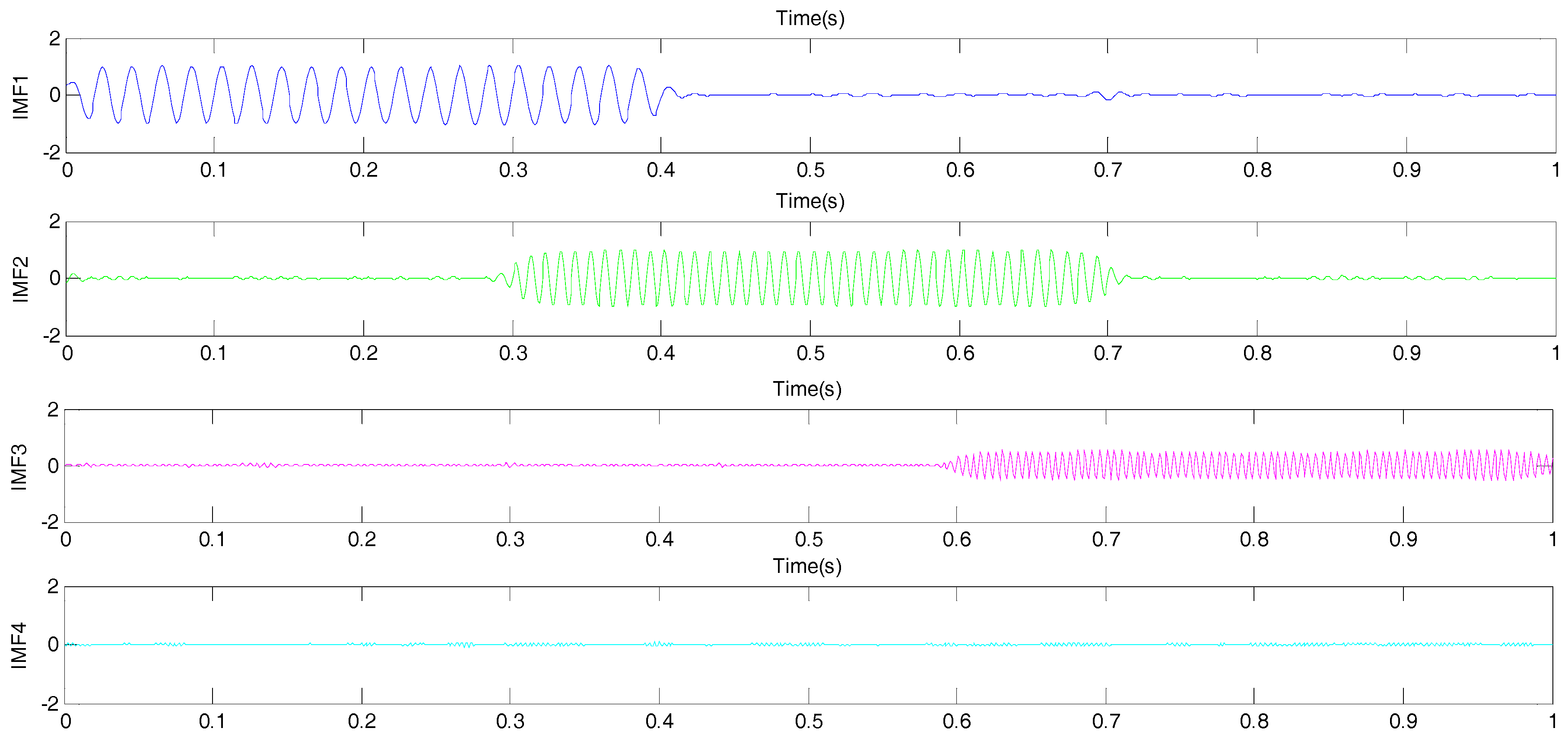
To verify the validity of the VMD algorithm, we used this method to decompose the synthetic data. The synthetic data consisted of four basic data sets, all of which are non-stationary, nonlinear signals. Data 1, within 0~0.4 s, is a sine wave with amplitude value A = 1, frequency f = 50 Hz and A is 0 within 0.4~1 s; data 2, within 0.3~0.7 s, is a sine wave with amplitude value A = 1, frequency f = 100 Hz, and A value is 0 during 0~0.3 s and 0.7~1 s; data 3, within 0.6~1 s, is a sine wave with amplitude value A = 0.5, frequency f = 200 Hz, and A is 0 within 0~0.6 s; data 4 is random noise. The synthetic signal is shown in Figure 1.
The synthetic data was processed by the VMD method, with k as 4, and the obtained result is shown in Figure 2. It was found that the four components obtained by the decomposition correspond well to the original data 1–4, and their abrupt points and waveforms remain consistent. IMF1 corresponds to data 1, IMF2 corresponds to data 2, IMF3 corresponds to data 3, and IMF4 corresponds to data 4 (random noise data).
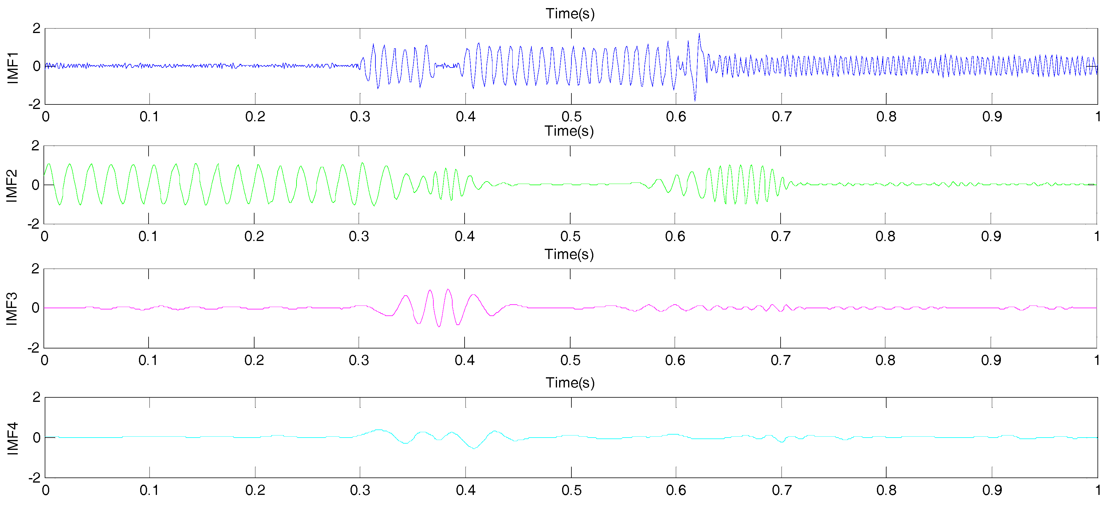
To prove the advantages of the VMD method, this paper selected the EMD method to make a comparison, which is an adaptive signal analysis method suitable for non-stationary, nonlinear signals. Based on the features of the signal, it automatically extracts the intrinsic modal function (IMF) of the signal. The specific principle can be found in [12,13,14]. This section uses the EMD method to decompose the synthetic data in Figure 1, and the results are displayed in Figure 3. It is obvious that the correspondence between the four IMF components obtained by EMD and the original basic data 1–4 is bad, and the purpose of decomposing the synthetic data is not achieved. The effect of EMD is inferior to that of the VMD method.
The test results of VMD and EMD methods on the synthetic data were compared, and the comparison shows that the VMD method not only has a strict mathematical foundation, but also has the following advantages: (1) the algorithm is more competent than traditional EMD methods; (2) the decomposition effect of the non-stationary, nonlinear model is brilliant, and the result is more accurate; (3) it could overcome the modal aliasing shortcoming of the EMD method; (4) the noise immunity of the VMD is raised.
3.2. Processing Simulated Ice-Penetrating Radar Data with VMD
To verify the noise reduction effect of the VMD method on the ice-penetrating radar signal, this part used the VMD method to test the simulated ice-penetrating radar data. First, a simple ice sheet permittivity model and conductivity model were established. Then, the forward modeling was carried out to get the simulated ice-penetrating data. Finally, the VMD method was employed to decompose and reconstruct the analog signal.
3.2.1. Ice-Penetrating Radar Forward Simulation
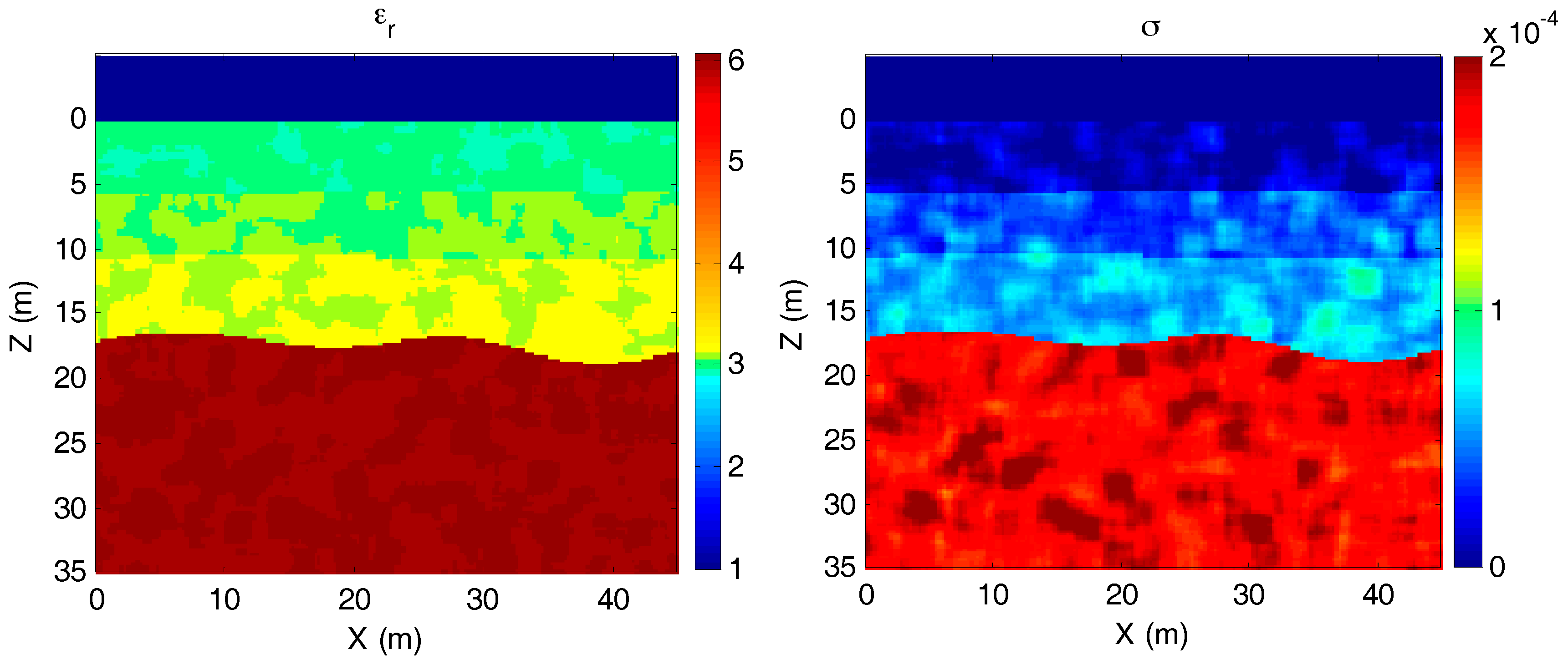
The model consists of air, ice sheet, subglacial bedrock and four interfaces (one ice rock interface, one air ice interface and two ice inner layer interfaces) and the ice sheet includes three ice inner layers. Utilizing the available resources, a small simulation model was set up. The size of the model was set to 45 m × 40 m, but the ice surface, as a reference surface, was 0 m, and the air layer was 5 m thick. The geometric parameters and electrical parameters set by the model are shown in Table 1. The electrical parameter setting is primarily in line with the article [33]. In order to increase the noise ratio in the simulation data, the random medium was considered. Finally, the permittivity model and the conductivity model as shown in Figure 4 were achieved.
The forward modeling was carried out for the above model using the time domain finite difference method (FDTD) [34,35,36]. The antenna center frequency was 300 MHz, the time window 400 ns, the sampling interval 0.101 ns, mesh size 0.05 m × 0.05 m, the number of collecting traces 121, and the distance interval 0.375 m. The height of the acquisition position was 5 m from the ground, and the offset of the antenna was 0.1 m.
Figure 5 is the ice-penetrating radar profile acquired by the simulation, and the 43rd trace is shown in Figure 6. The reflection information in Figure 5 is not so obvious, because the energy of the direct wave is too strong and the information below the ice surface is badly suppressed. Therefore, gain and direct wave subtracting processing were performed on the data, and the processed section is shown in Figure 7. The 43rd trace is shown in Figure 8. From the treated profile and the single trace, the interfaces between the ice inner layers and the ice rock can be seen, but the interference noise is also strengthened.
3.2.2. Processing Simulated Data with VMD
The data below the ice surface was used as test data (Figure 9a) and was processed by VMD. With k equal to 5, VMD was performed to obtain the five IMF components in Figure 9b–f. It is easy to see that IMF1, IMF3 and IMF4 are the main noise components, and IMF2 and IMF5 are the main components with useful information.
In order to quantitatively measure the useful information each IMFs contains, we calculated the correlation coefficient between each IMF and test data. We only added a random medium to the simulated data, so the noise was primarily generated by the random medium. Small noise proportion and mainly useful information allows the author to use the correlation coefficient between IMFs and test data as the quantitative standard. If the correlation coefficient is large, meaning the IMF contains more useful information, the IMF cannot be eliminated; if the correlation number is small, meaning the IMF contains less useful information, we can decide to eliminate the IMF or not according to the IMF profile (in this paper, the IMFs were selected for reconstruction when the correlation coefficient between them and input data was bigger than 0.6). The calculation results are shown in the Table 2.
Therefore, the composite profile of the components IMF2 and IMF5 was obtained as shown in Figure 10. From the comparison of Figure 9a with Figure 10 we can see the latter is apparently clearer. The VMD method eliminates a large amount of noise. Through the elimination and recombination, the signal-to-noise ratio of the whole data set was significantly enhanced.
4. Processing and Interpretation of Antarctic Ice-Penetrating Radar Data
4.1. Analysis and Processing of Antarctic Ice-Penetrating Radar Data
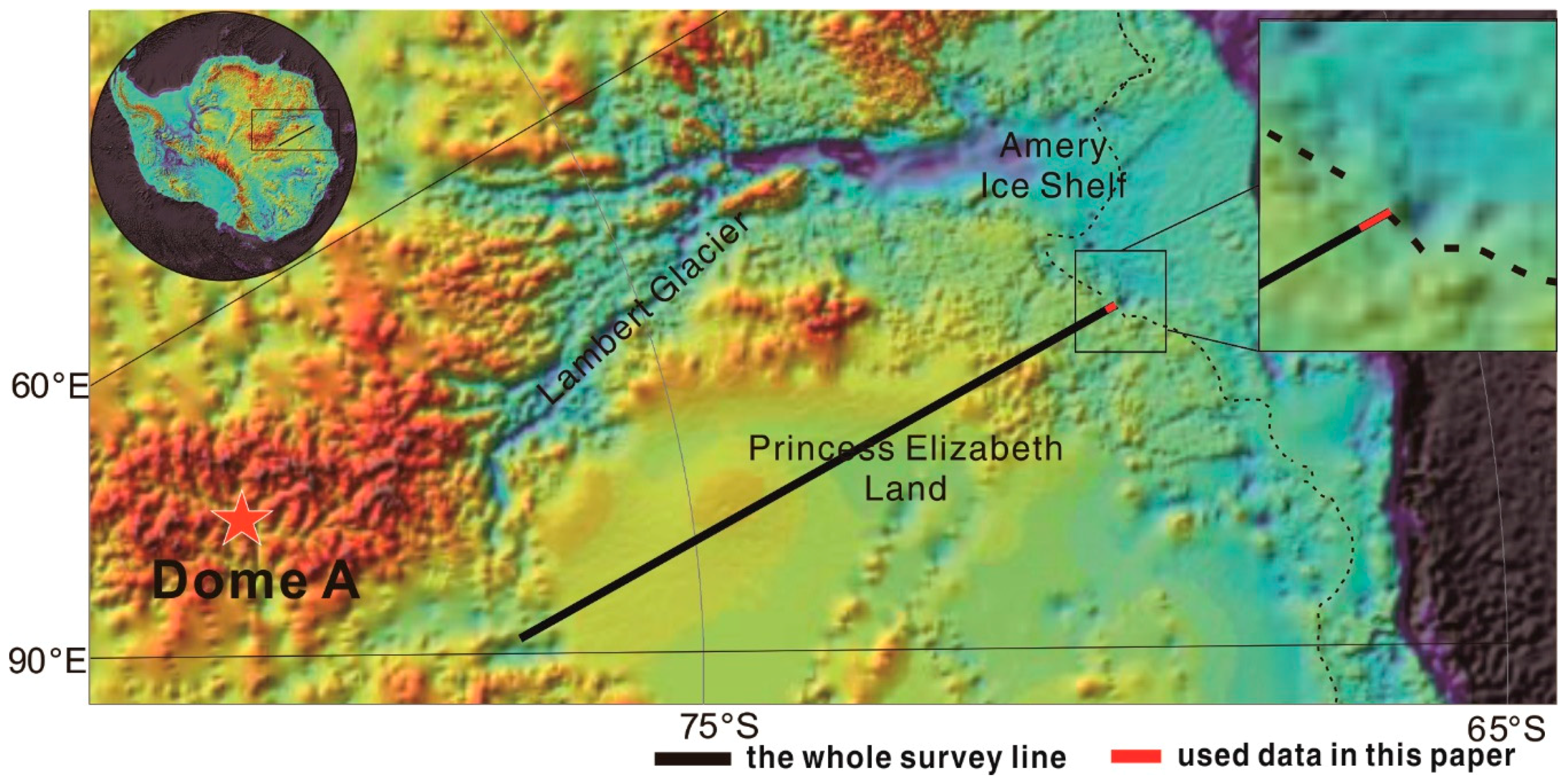
The data in this section is a segment of a survey line (as shown in Figure 11) in the real data collected by the airborne HiCARS radar system (Figure 12) during the 32nd Chinese Antarctic scientific research survey in 2015 [37]. There are 1000 traces, each of which has 2000 sampling points. The sampling frequency was 50 MHz and the center frequency was 60 MHz. After DC removal, band-pass filtering (10–20–150–300 MHz), migration by constant velocity (velocity was 0.167 m/ns) and delete mean trace, the VMD processing was carried out on the airborne radar data.
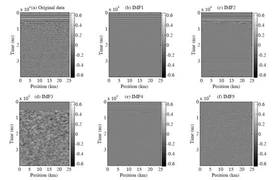
Although the real data used (as shown in Figure 13) has been processed by conventional processing, its signal-to-noise ratio is still low, and there is a large amount of interference noise, which causes the isochronous layer in the ice being blurred. First, the 405th trace (as shown in Figure 14a) was used as the test trace to be processed by the VMD method, after which we got five IMF components as shown in the Figure 14b–f, where k is 5.
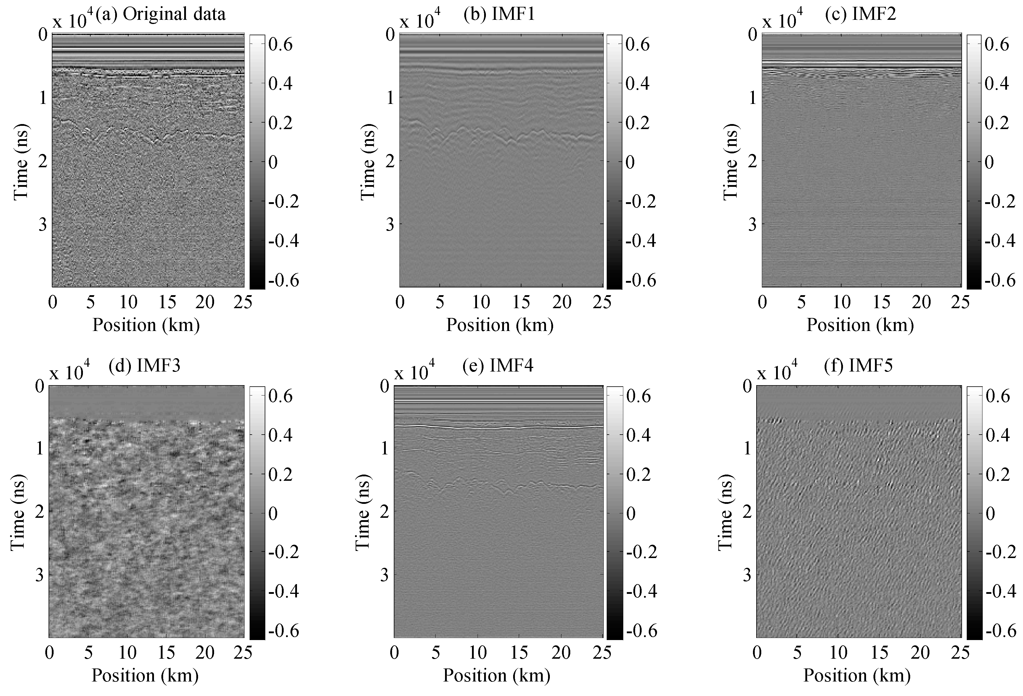
Subsequently, the entire profile was processed by VMD to obtain five IMF profiles as shown in Figure 15. From the figure, it can be seen that IMF2, IMF3 and IMF5 are the ones mainly containing noise, while the IMF1 and IMF4 components mainly contain ice rock interface and ice internal layer reflection information.
Similarly, in order to quantitatively measure the useful information contained in each of the IMFs, we also calculated the correlation coefficient between each IMF and the original data. For an effective real data, useful information should take up the main part, and noise a small one. Thus, it is acceptable that the author took the correlation coefficient between the IMFs and original data as a quantitative standard. The calculation results are shown in Table 3.
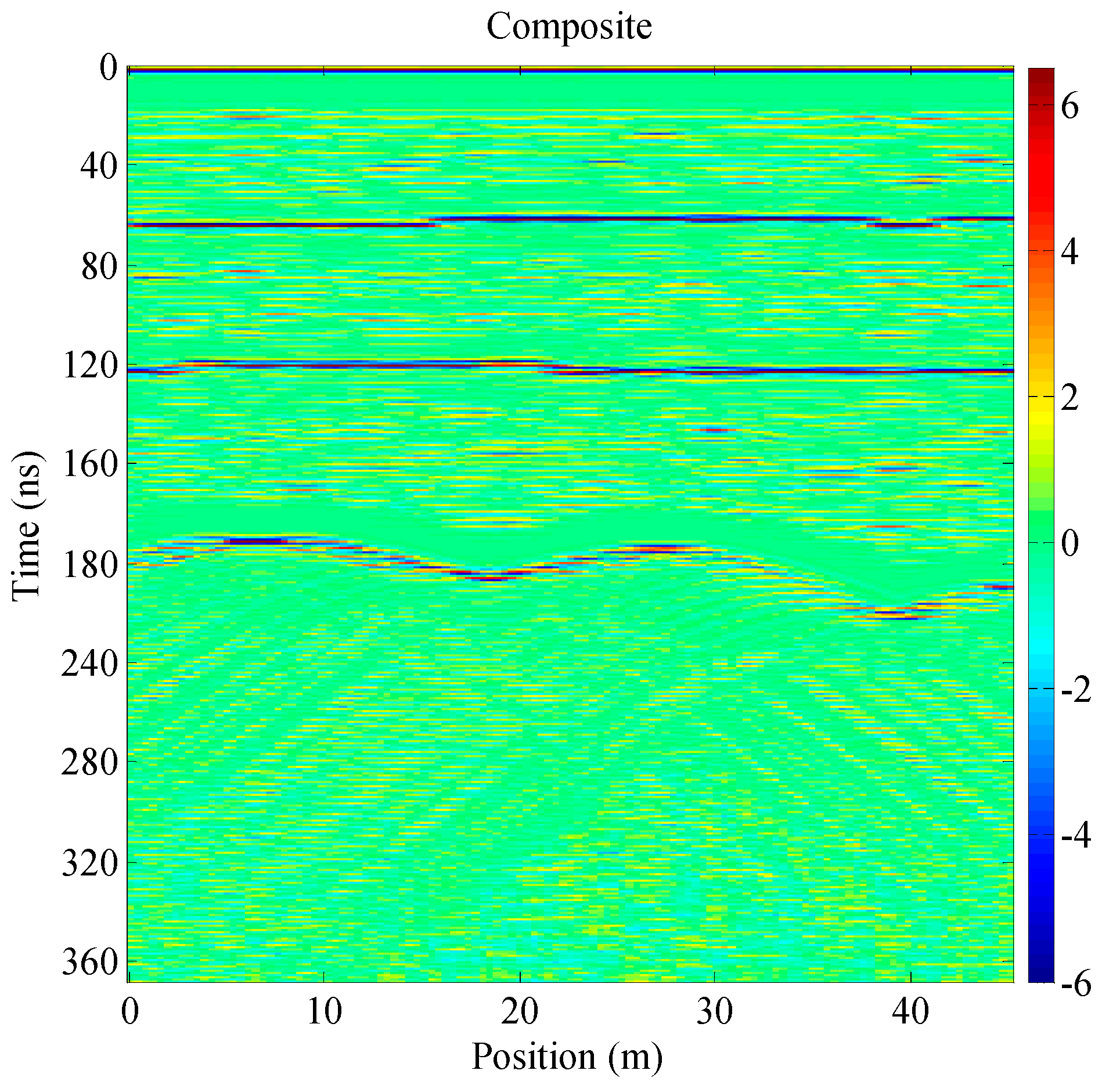
It was found that the correlation coefficient obtained by calculation is consistent with the judgement we made according to the IMF profiles. According to the display of the IMF components, IMF1 and IMF4 were combined to acquire the composite profile shown in Figure 16. For comparison, the original data profile is placed beside the composite profile. Obviously, the composite section reconstructed by VMD is clearer than the original, the interface between the isochronous layer and the bedrock is more prominent, and the noise is greatly reduced, which effectively improves the signal-to-noise ratio. The peak signal-to-noise ratio (PSNR) was calculated to quantify the noise reduction ability of VMD to the real data. The PSNR of the original data was 15.39 dB and the PSNR of the composite was 20.27 dB. It further proves that the VMD method has a demonstrative advantage in noise reduction of ice-penetrating radar data.
4.2. Interpretation of Data
The distribution and structural characteristics of the isochronous layers inside the ice sheet reflect the historical evolution of ice deposition and ice flow. It can be used for selecting deep ice core drilling sites, understanding the ice sheet dynamic processes, estimating ice sheet mass balance and assessing ice sheet stability [38]. From the study of the Antarctic and Arctic ice sheets, we know there are three main mechanisms for the formation of the isochronous layers of the ice sheet: (a) in the upper 700–900 m of the ice sheet, reflective layers are mainly caused by ice density changes; (b) some reflective layers of ice may be induced by the aerosol material from volcanic eruptions; (c) other reflection layers resulted from the anisotropic crystal-orientation fabric and are largely found in the deep ice layer, which is deeper than 900 m [39,40,41].
Ice core data shows that the ice density of the Antarctic ice sheet varies with different depths, and the density and conductive changes feature isochronous quality [42,43]. In the upper part of the ice sheet, the ice first changes from the mechanical compression stage to the plastic deformation and recrystallization stage, and the density increases rapidly as the density reaches a critical value of 500 kg/m−3. Below that, the rate of density increase slows down until the density reaches the critical density value of 830 kg/m−3, where the air in the ice becomes bubbles. Finally, as the depth increases, the bubbles in the ice enter the lattice and become a cage hydrate. After approaching 917 kg/m−3, the ice density tends to be stable and uniform [41,44,45].
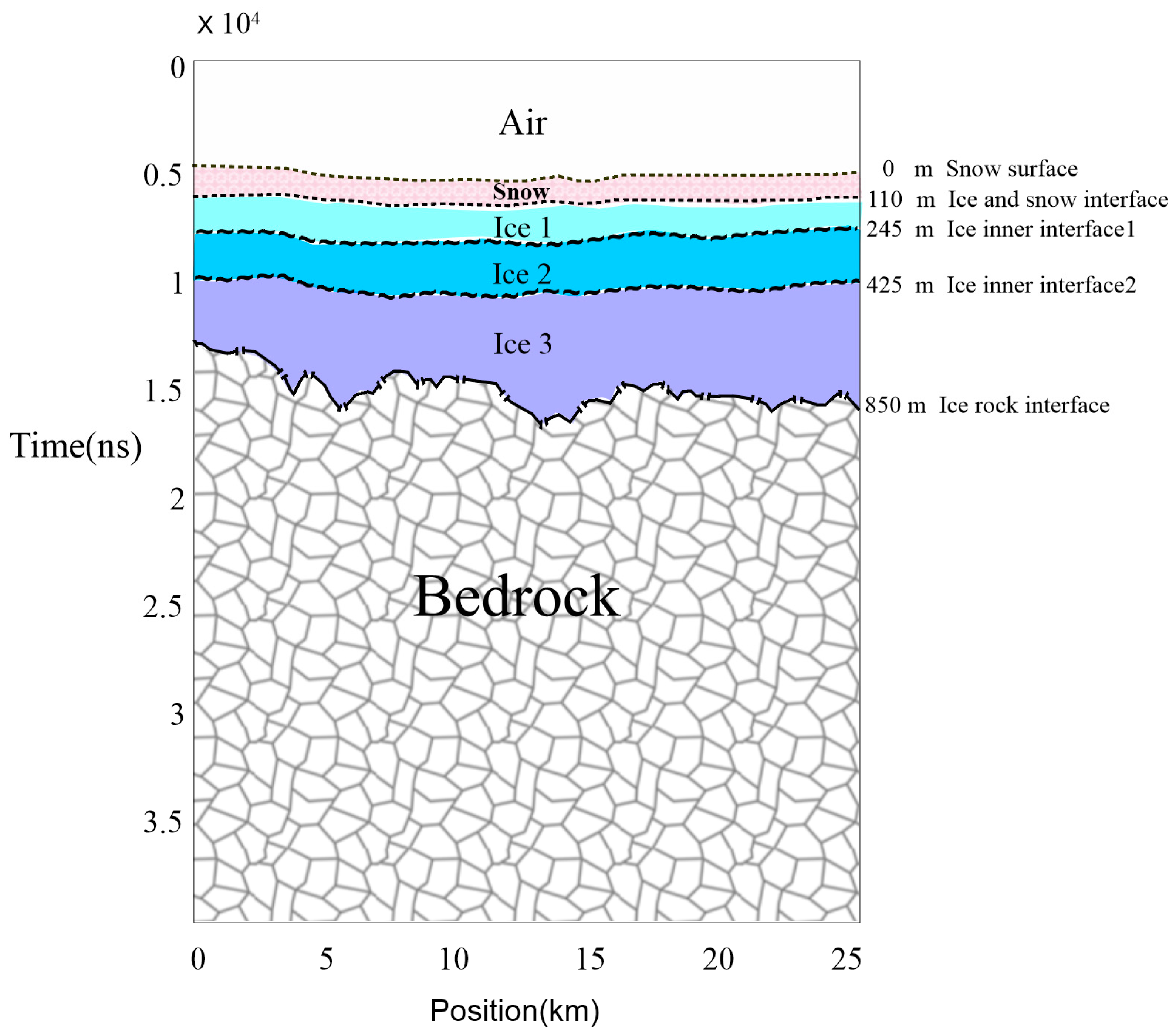
In general, the air layer, snow layer, ice layer and bedrock layer can be distinguished in the airborne IPR data profile. From the information provided by the composite profile, we can see five distinct and continuous electromagnetic wave reflection interfaces caused by differences in conductivity or permittivity. We set the depth of the first reflective interface to 0 m. According to the time-depth conversion, the average depth from top to bottom is 110 m, 245 m, 425 m and 850 m. Obviously, the first reflective interface corresponds to the snow surface. Below the snow surface, there will be a strong reflection signal at the ice-ice interface caused by the electrical difference between snow (the density of Antarctic snow is about 300 kg/m−3) and ice. In light of the propagation speed of electromagnetic waves in the Antarctic snow, the depth of the second interface is 110 m, which is consistent with the average snow depth data of the area, so the second interface is predicated to be the interface of ice and snow [46]. The depth of the third and fourth reflective interfaces (245 m and 425 m) are both less than 700 m. According to the previously mentioned layer formation mechanisms, it is currently assumed that these two interfaces are created by the difference in the two critical densities of ice, but the specific causes of this need to be supported by the study of ice cores in the area. The fifth reflective interface (850 m) is an ice rock interface.
In summary, we divided the airborne ice-penetrating radar data profile into four layers, including air, snow, ice and bedrock layers. Moreover, the ice layers are divided into three ice inner layers as shown in Figure 17. The snow surface, ice and snow interface, ice inner layer reflection interface and ice rock interface are also described.
5. Conclusions
In this paper, a novel mode decomposition technique, VMD, is applied to the noise reduction processing of ice-penetrating radar data, and the ideal results are obtained. The VMD algorithm uses a completely non-recursive approach to achieve frequency domain decomposition of signals and noise. It boasts the advantages of strong decomposition capability, excellent anti-noise performance and fast processing speed. The real ice-penetrating radar data processing example shows that the method could effectively improve the signal-to-noise ratio of ice-penetrating radar data in the polar regions and enhance the continuity of the event. It offers an effective means for obtaining more abundant information inside the ice sheet and bedrock, which is beneficial for later interpretation and can be widely used in the noise reduction of ice-penetrating radar data processing. From the processed data, four layers and five interfaces are clearly interpreted by combining it with general ice sheet knowledge.
Author Contributions
Methodology, S.C.; software, S.C.; validation, S.L., X.T. and J.G.; formal analysis, S.L.; resources, X.T.; writing—original draft preparation, S.C.; writing—review and editing, K.L., L.Z. and S.C.; supervision, S.L., X.T. and J.G.
Funding
This study is supported by the National Natural Science Foundation of China (Nos. 41876230, 41876227, 41376192) and the Chinese Polar Environmental Comprehensive Investigation and Assessment Programs (CHIANRE 2017-01-01/CHIANRE2017-04-01/CHIANRE2017-04-03).
Acknowledgments
We express our appreciation to the Polar Research Institute of China for data support.
Conflicts of Interest
The authors declare no conflict of interest.
References
- Qin, D.H.; Kang, S.C. Present process of glacier and global climatic and environmental change. Earth Sci. Front. 1997, 4, 85–94. (In Chinese) [Google Scholar]
- Allison, I.; Alley, R.B.; Fricker, H.A.; Thomas, R.H.; Warner, R.C. Ice sheet mass balance and sea level. Antarct. Sci. 2009, 21, 413–426. [Google Scholar] [CrossRef] [Green Version]
- Deconto, R.M.; Pollard, D. Contribution of Antarctica to past and future sea-level rise. Nature 2016, 531, 591–597. [Google Scholar] [CrossRef]
- Zhang, X.P.; Sun, B.; Wang, B.B.; Tang, X.Y.; Tian, G. Radar Detection of Characteristics and Distribution of Isochronous Ice Layer in Antarctic Ice Sheet. In Proceedings of the Chinese Geophysical Society Annual Conference, Hangzhou, China, 15–19 October 2006. (In Chinese). [Google Scholar]
- Shepherd, A.; Ivins, E.R.; Rignot, E.; Smith, B.; Broeke, M.R.V.D.; Velicogna, I.; Whitehouse, P.L.; Briggs, K.; Joughin, I.; Krinner, G.; et al. Mass balance of the Antarctic Ice Sheet from 1992 to 2017. Nature 2018, 558, 219–222. [Google Scholar] [Green Version]
- Evans, S. Radio techniques for the measurement of ice thickness. Pol. Rec. 1963, 11, 406–410. [Google Scholar] [CrossRef]
- Plewes, L.A.; Hubbard, B. A review of the use of radio-echo sounding in glaciology. Prog. Phys. Geogr. 2001, 25, 203–236. [Google Scholar] [CrossRef]
- Bogorodskiy, V.V.; Bentley, C.R.; Gudmandsen, P. Radioglaciology; Kluwer: Dordrecht, The Netherlands, 1985. [Google Scholar]
- Cui, X.B.; Sun, B.; Zhang, X.P.; Zhang, D.; Li, X.; Tang, X.; Tian, G. A review of ice radar’s technical development in polar ice sheet investigation. Chin. J. Polar Res. 2009, 21, 322–335. (In Chinese) [Google Scholar]
- Bingham, R.G.; Siegert, M.J. Radio-echo sounding over polar ice masses. J. Environ. Eng. Geophys. 2007, 12, 47–62. [Google Scholar] [CrossRef]
- Tzanis, A. Detection and extraction of orientation-and-scale-dependent information from two-dimensional GPR data with tuneable directional wavelet filters. J. Appl. Geophys. 2013, 89, 48–67. [Google Scholar] [CrossRef]
- Rilling, G.; Flandrin, P.; Gonçalvès, P. On empirical mode decomposition and its algorithms. In Proceedings of the IEEE-Eurasip Workshop Nonlinear Signal Image Process, c(NSIP), Trieste, Italy, 8–11 June 2003; Volume 3, pp. 8–11. [Google Scholar]
- Wang, T. Research on EMD Algorithm and Its Application in Signal Denoising; Harbin Engineering University: Harbin, China, 2010. (In Chinese) [Google Scholar]
- Huang, N.E.; Shen, Z.; Long, S.R.; Wu, M.C.; Shih, H.H.; Zheng, Q.; Yen, N.; Tung, C.C.; Liu, H.H. The empirical mode decomposition and the Hilbert spectrum for nonlinear and non-stationary time series analysis. Proc. R. Soc. A Math. Phys. Eng. Sci. 1998, 454, 903–995. [Google Scholar] [CrossRef]
- Partyka, G.; Gridley, J.; Lopez, J. Interpretational applications of spectral decomposition in reservoir characterization. Lead. Edge 1999, 18, 353–360. [Google Scholar] [CrossRef] [Green Version]
- Chakraborty, A.; Okaya, D. Frequency-time decomposition of seismic data using wavelet-based methods. Geophysics 1995, 60, 1906–1916. [Google Scholar] [CrossRef]
- Odebeatu, E.; Zhang, J.; Chapman, M.; Liu, E.; Li, X.Y. Application of spectral decomposition to detection of dispersion anomalies associated with gas saturation. Lead. Edge 2006, 25, 206–210. [Google Scholar] [CrossRef]
- Li, Y.; Zheng, X. Spectral decomposition using Wigner-Ville distribution with applications to carbonate reservoir characterization. Lead. Edge 2008, 27, 1050–1057. [Google Scholar] [CrossRef]
- Wang, Y.H.; Yeh, C.H.; Young, H.W.V.; Hu, K.; Lo, M.T. On the computational complexity of the empirical mode decomposition algorithm. Phys. A Stat. Mech. Its Appl. 2014, 400, 159–167. [Google Scholar] [CrossRef]
- Zhang, L.; Zeng, F.Z.; Li, J.; Lin, J.; Hu, Y.; Wang, X.; Sun, X. Simulation of the Lunar Regolith and Lunar-Penetrating Radar Data Processing. IEEE J. Sel. Top. Appl. Earth Obs. Remote Sens. 2018, 11, 655–663. [Google Scholar] [CrossRef]
- Zhang, L.; Zeng, F.Z.; Li, J.; Hu, Z.; Zhang, J. Lunar Penetrating Radar Data Processing and Analysis Based on CEEMD. In Proceedings of the 2018 17th International Conference on Ground Penetrating Radar (GPR), Rapperswil, Switzerland, 18–21 June 2018. [Google Scholar]
- Dragomiretskiy, K.; Zosso, D. Variational mode decomposition. IEEE Trans. Signal Process. 2014, 62, 531–544. [Google Scholar] [CrossRef]
- Dragomiretskiy, K.; Zosso, D. Two-dimensional variational mode decomposition. Energy Minimization Methods Comput. Vis. Pattern Recognit. 2015, 8932, 197–208. [Google Scholar]
- Xue, Y.J.; Cao, J.X.; Wang, D.X.; Du, H.K.; Yao, Y. Application of the Variational-Mode Decomposition for Seismic Time–frequency Analysis. IEEE J. Sel. Top. Appl. Earth Obs. Remote Sens. 2017, 9, 3821–3831. [Google Scholar] [CrossRef]
- Zhang, X.; Nilot, E.; Feng, X.; Ren, Q.; Zhang, Z. IMF-Slices for GPR Data Processing Using Variational Mode Decomposition Method. Remote Sens. 2018, 10, 476. [Google Scholar] [CrossRef]
- Hoeher, P.A.; Kaiser, S.; Robertson, P. Two-dimensional pilot-symbol-aided channel estimation by Wiener filtering. In Proceedings of the International Conference on Acoustics, Speech, and Signal Processing, Munich, Germany, 21–24 April 1997; pp. 1845–1848. [Google Scholar]
- Buades, A.; Coll, B.; Morel, J. A non-local algorithm for image denoising. Comput. Vis. Pattern Recogn. 2005, 2, 60–65. [Google Scholar]
- Feng, D.S.; Chen, C.S.; Yu, K. Signal Enhancement and Complex Signal Analysis of GPR Based on Hilbert-Huang Transform. Lect. Notes Electr. Eng. 2011, 99, 375–384. [Google Scholar]
- Daubechies, I.; Lu, J.; Wu, H.-T. Synchrosqueezed wavelet transforms: An empirical mode decomposition-like tool. Appl. Comput. Harmon. Anal. 2011, 30, 243–261. [Google Scholar] [CrossRef] [Green Version]
- Gilles, J. Empirical wavelet transform. IEEE Trans. Signal Process. 2013, 61, 3999–4010. [Google Scholar] [CrossRef]
- Rockafellar, R.T. A dual approach to solving nonlinear programming problems by unconstrained optimization. Math. Program 1973, 5, 354–373. [Google Scholar] [CrossRef] [Green Version]
- Bertsekas, D.P. Constrained optimization and Lagrange Multiplier methods. In Computer Science and Applied Mathematics; Academic Pr: Boston, MA, USA, 1982; Volume 1. [Google Scholar]
- MacGregor, J.A.; Winebrenner, D.P.; Conway, H.; Matsuoka, K.; Mayewski, P.A.; Clow, G.D. Modeling englacial radar attenuation at Siple Dome, West Antarctica, using ice chemistry and temperature data. J. Geophys. Res. Earth Surf. 2007, 112, 1–14. [Google Scholar] [CrossRef]
- Liu, S.X.; Zeng, Z.F.; Xu, B. FDTD Simulation of Ground Penetrating Radar Signal in 3-Dimensional Dispersive Medium. J. Jilin Univ. (Earth Sci. Ed.) 2006, 36, 123–127. (In Chinese) [Google Scholar]
- Li, J.; Zeng, Z.F.; Wu, F.S.; Lin, H. Study of three dimension high-order FDTD simulation for GPR. Chin. J. Geophys. 2010, 53, 974–981. (In Chinese) [Google Scholar]
- Feng, D.S.; Chen, C.S.; Dai, Q.W. GPR numerical simulation of full wave field based on UPML boundary condition of ADI-FDTD. Chin. J. Geophys. 2010, 53, 2484–2496. (In Chinese) [Google Scholar]
- Cui, X.B.; Wang, T.T.; Sun, B.; Tang, X.; Guo, J. Chinese radioglaciological studies on the Antarctic ice sheet: Progress and prospects. Adv. Polar Sci. 2017, 28, 161–170. [Google Scholar]
- Jacobel, R.W.; Hodge, S.M. Radar Internal Layers from the Greenland Summit. Geophys. Res. Lett. 1995, 22, 587–590. [Google Scholar] [CrossRef]
- Fujita, S.; Maeno, H.; Uratsuka, S.; Furukawa, T.; Mae, S.; Fujii, Y.; Watanabe, O. Nature of radio echo layering in the Antarctic ice sheet detected by a two-frequency experiment. J. Geophys. Res. Solid Earth 1999, 104, 13013–13024. [Google Scholar] [CrossRef]
- Yang, S.H.; Gu, Q.M.; Yun, Y.; Cui, X.B.; Tang, X.Y. A review of the use of ice penetrating radar to diagnose the subglacial environments. Chin. J. Polar Res. 2016, 28, 277–286. (In Chinese) [Google Scholar]
- Tang, X.Y.; Sun, B.; Cui, X.B. Review of research progress of internal radar isochronous layers in Antarctic ice sheet. Chin. J. Polar Res. 2015, 27, 104–114. (In Chinese) [Google Scholar]
- Vaughan, D.G.; Anderson, P.S.; King, J.C.; Mann, G.W.; Mobbs, S.D.; Ladkin, R.S. Imaging of firn isochrones across an Antarctic ice rise and implications for patterns of snow accumulation rate. J. Glaciol. 2004, 50, 413–418. [Google Scholar] [CrossRef]
- Eisen, O.; Nixdorf, U.; Wilhelms, F.; Miller, H. Age estimates of isochronous reflection horizons by combining ice core, survey, and synthetic radar data. J. Geophys. Res. 2004, 109. [Google Scholar] [CrossRef] [Green Version]
- Herron, M.M.; Langway, C.C. Firn densification: An empirical model. J. Glaciol. 1980, 25, 373–385. [Google Scholar] [CrossRef]
- Cuffey, K.M.; Paterson, W.S.B. The Physics of Glaciers, 4th ed.; Academic Press: Cambridge, MA, USA, 2010; pp. 11–25. [Google Scholar]
- Grima, C.; Blankenship, D.D.; Young, D.A.; Schroeder, D.M. Surface slope control on firn density at Thwaites Glacier, West Antarctica: Results from airborne radar sounding. Geophys. Res. Lett. 2014, 41, 6787–6794. [Google Scholar] [CrossRef]
Figure 1.
(a) synthetic data; (b) data 1; (c) data 2; (d) data 3; (e) data 4.

Figure 2.
Intrinsic Mode Function (IMF) components obtained by decomposing synthetic data with Variational Mode Decomposition (VMD).
Figure 2.
Intrinsic Mode Function (IMF) components obtained by decomposing synthetic data with Variational Mode Decomposition (VMD).

Figure 3.
IMF components obtained by decomposing synthetic data with Empirical Mode Decomposition (EMD).
Figure 3.
IMF components obtained by decomposing synthetic data with Empirical Mode Decomposition (EMD).

Figure 4.
Relative permittivity model (left) and conductivity model (right).

Figure 5.
Simulated data profile.

Figure 6.
The 43rd trace of simulated data.

Figure 7.
Processed simulated data profile.

Figure 8.
The 43rd trace of processed simulated data.

Figure 9.
Test data and IMF components obtained by decomposing the simulated data with VMD. (a) Test data, (b) IMF1, (c) IMF2, (d) IMF3, (e) IMF4, (f) IMF5.
Figure 9.
Test data and IMF components obtained by decomposing the simulated data with VMD. (a) Test data, (b) IMF1, (c) IMF2, (d) IMF3, (e) IMF4, (f) IMF5.

Figure 10.
Combination of IMF2 and IMF5 of the simulated radar data.

Figure 11.
The data collection location of airborne ice-penetrating radar in the Antarctic. The background image is badmap2 bed elevation.
Figure 11.
The data collection location of airborne ice-penetrating radar in the Antarctic. The background image is badmap2 bed elevation.

Figure 12.
The first fixed-wing airplane Snow Eagle 601 deployed by China for Antarctic survey with airborne geophysical instruments including Airborne HiCARS radar system [37].
Figure 12.
The first fixed-wing airplane Snow Eagle 601 deployed by China for Antarctic survey with airborne geophysical instruments including Airborne HiCARS radar system [37].

Figure 13.
Data profile after conventional data processing, where the red line represents the position of the 45th trace.
Figure 13.
Data profile after conventional data processing, where the red line represents the position of the 45th trace.

Figure 14.
Test trace and IMF components obtained by decomposing airborne ice-penetrating radar single trace data with VMD. (a) Test trace, (b) IMF1, (c) IMF 2, (d) IMF3, (e) IMF4, (f) IMF5.
Figure 14.
Test trace and IMF components obtained by decomposing airborne ice-penetrating radar single trace data with VMD. (a) Test trace, (b) IMF1, (c) IMF 2, (d) IMF3, (e) IMF4, (f) IMF5.

Figure 15.
Original data and IMF components obtained by VMD. (a) Original data, (b) IMF1, (c) IMF2, (d) IMF3, (e) IMF4, (f) IMF5.
Figure 15.
Original data and IMF components obtained by VMD. (a) Original data, (b) IMF1, (c) IMF2, (d) IMF3, (e) IMF4, (f) IMF5.

Figure 16.
(a) Original data profile; (b) Composite profile.

Figure 17.
Resulting profile.


Table 1.
Two-dimensional random medium model parameters.
| Composition | Interface | Average Depth of the Interface (m) | Ice Inner Layer | Average Relative Permittivity ɛr | Average Conductivity σ(s/m) |
|---|---|---|---|---|---|
| Air | - | - | 1 | 0 | |
| Air ice interface | 0 | ||||
| Ice sheet | I | 3.00 | 0.00001 | ||
| Ice inner layer interface 1 | 5 | ||||
| II | 3.07 | 0.00004 | |||
| Ice inner layer interface 2 | 10 | ||||
| III | 3.15 | 0.00006 | |||
| Ice rock interface | 17.5 | ||||
| Bedrock | - | 6 | 0.00018 | ||
| - | |||||
Table 2.
Correlation coefficient table between IMFs and test data.
| IMFs | IMF1 | IMF2 | IMF3 | IMF4 | IMF5 |
|---|---|---|---|---|---|
| Correlation Coefficient | 0.5059 | 0.6375 | 0.3841 | 0.3529 | 0.7839 |
Table 3.
Correlation coefficient table between IMFs and original data.
| IMFs | IMF1 | IMF2 | IMF3 | IMF4 | IMF5 |
|---|---|---|---|---|---|
| Correlation Coefficient | 0.6313 | 0.2996 | 0.2230 | 0.6819 | 0.2412 |
© 2019 by the authors. Licensee MDPI, Basel, Switzerland. This article is an open access article distributed under the terms and conditions of the Creative Commons Attribution (CC BY) license (http://creativecommons.org/licenses/by/4.0/).
Share and Cite
MDPI and ACS Style
Cheng, S.; Liu, S.; Guo, J.; Luo, K.; Zhang, L.; Tang, X. Data Processing and Interpretation of Antarctic Ice-Penetrating Radar Based on Variational Mode Decomposition. Remote Sens. 2019, 11, 1253. https://doi.org/10.3390/rs11101253
AMA Style
Cheng S, Liu S, Guo J, Luo K, Zhang L, Tang X. Data Processing and Interpretation of Antarctic Ice-Penetrating Radar Based on Variational Mode Decomposition. Remote Sensing. 2019; 11(10):1253. https://doi.org/10.3390/rs11101253
Chicago/Turabian StyleCheng, Siyuan, Sixin Liu, Jingxue Guo, Kun Luo, Ling Zhang, and Xueyuan Tang. 2019. "Data Processing and Interpretation of Antarctic Ice-Penetrating Radar Based on Variational Mode Decomposition" Remote Sensing 11, no. 10: 1253. https://doi.org/10.3390/rs11101253
Note that from the first issue of 2016, this journal uses article numbers instead of page numbers. See further details here.