Article

Coastal Waveform Retracking in the Slick-Rich Sulawesi Sea of Indonesia, Based on Variable Footprint Size with Homogeneous Sea Surface Roughness

1
School of Marine Science and Environment Engineering, Dalian Ocean University, Dalian 116023, China
2
Research Institute for Applied Mechanics, Kyushu University, Fukuoka 8168580, Japan
3
Dalian Marine Environmental Monitoring Station of Chinese State Oceanic Administration, Dalian 116015, China
*
Author to whom correspondence should be addressed.
Remote Sens. 2019, 11(11), 1274; https://doi.org/10.3390/rs11111274
Submission received: 29 March 2019 / Revised: 9 May 2019 / Accepted: 24 May 2019 / Published: 29 May 2019
(This article belongs to the Special Issue Advances in Satellite Altimetry and Its Application)

Abstract

:
Waveforms of radar altimeters are often corrupted due to heterogeneous sea surface roughness within footprints, such as slicks. In past studies, subwaveform retrackers such as the adaptive leading edge subwaveform retracker (ALES) which use only a section of the waveform have been proposed. However, it is difficult to choose a reasonable estimation window from an individual waveform. In the present study, a post-processed subwaveform retracker is proposed which identifies the waveforms of surrounding along-track points. The size of the estimation window is variable and is determined to keep the sea surface roughness within the corresponding footprint homogeneous. The method was applied to seven years of 20 Hz Jason-2 altimeter data over the slick-rich Sulawesi Sea of Indonesia and compared with ALES and sensor geophysical data record (SGDR) products. The standard deviation of the sea surface dynamic heights was around 0.13 m, even without spatial smoothing or some geophysical corrections. This is only 75% and 25% of the ALES and SGDR results, respectively. Moreover, all retrievals of the range, SWH, and sigma0 include less outliers than the other products. These results indicate that the variable estimation windows determined in the present study can adapt well to the variation of sea surface roughness.

Graphical Abstract

1. Introduction

Radar altimeters transmit pulses towards the sea at a nadir and then receive the echoes reflected from the sea surface within an altimeter footprint. The received echoes are sampled with a specific time resolution. The time series of the power of the samples is commonly referred to as a “waveform”, and each cell within a waveform is called a “gate”. Geophysical parameters, including the sea surface height (SSH), significant wave height (SWH), and the wind speed (related to backscatter coefficient, sigma0), are retrieved from the waveforms by a process called “retracking”. The so-called Brown mathematical model [1,2] is the standard model used for this process.
When surfaces are homogeneous within an altimeter footprint, a typical Brown-type waveform has a well-defined shape consisting of three parts: thermal noise, a fast-rising leading edge, and a decaying trailing edge. However, the waveform will be corrupted and deviate from the shape of the Brown waveform under heterogeneous surface conditions. The waveform corruption is particularly serious over coastal areas [3]. In recent years, the impact of contamination sources over coastal areas, like calm waters, ships, land masses, etc., on waveform retracking have been discussed [4,5]. Moreover, heterogeneous surfaces due to sea slicks are commonly observed even far from the coast in all previous radar altimeter missions. For example, about 6% of the Jason-1 measurements are corrupted by sea slicks [6].
Geophysical parameters cannot be correctly retrieved by applying the Brown model directly to entire corrupted waveforms. Therefore, several subwaveform retrackers have been proposed in recent years [7,8]. These retrackers use only a portion of the waveform trailing edge close to the leading edge, which is equivalent to reducing the size of the altimeter footprint. Hence, they can effectively reduce noise in the waveform trailing edge. However, the location of corrupted echoes in individual waveforms depends on the location of the contamination sources relative to the altimeter nadir track. Subwaveform retrackers may incorrectly estimate the geophysical parameters if corrupted echoes occur within the estimation window of subwaveform retrackers. Therefore, an ideal subwaveform retracker is needed to automatically adjust the length of the estimation window according to the uniformity of the sea surface.
An adapting leading edge subwaveform retracker (ALES) with an estimation window length proportional to the SWH estimation has been proposed in recent years [9]. The SWH-dependent estimation window aims to include all gates constituting the leading edge and only minimal gates of the trailing edge. Hence, it can retrack both open ocean and coastal data with the same accuracy without being subject to contamination in the trailing edge. However, the determination of the estimation window strongly depends on the SWH estimation of noisy individual waveforms.
Recently, Wang and Ichikawa proposed a post-processing retracking method to identify waveforms of along-track adjacent observations [
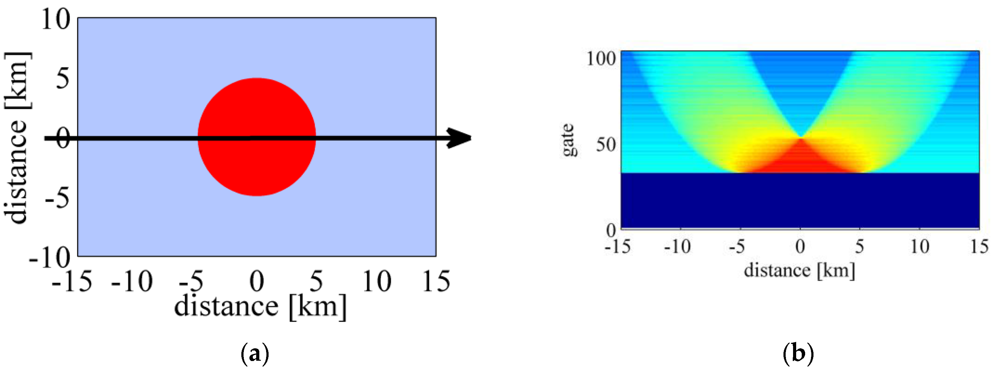
10]. Generally, significant echoes from a point target, such as a calm sea surface in a semi-closed bay, result in a parabolic signature in the sequential along-track waveforms (hereafter, referred to as echograms). By masking these parabolic shapes, the SSH information in the mid-latitudes (near Taiwan and the Tsushima Islands, Japan) were successfully retracked. However, corrupted echoes from wide-area sources, such as sea slicks, do not show as parabolas in echograms. The above method cannot be applied to bright echoes from point targets like a calm bay with a small area.
The present study proposes a subwaveform retracker which considers the possible effects of various corruption sources through automatic adjustment of the length of the estimation window. Different from the ALES retracker, the estimation window is no longer determined by a single waveform but depends on the footprint size with homogeneous sea surface roughness, using spatial restriction conditions in echograms.

2. Dataset

In past studies, the result of slick detection for the Jason-1 altimeter revealed a seasonal movement of sea slicks and found that slicks are present in the Northern Hemisphere during boreal summer and in the Southern Hemisphere during boreal winter [6]. In other words, sea slicks more often occur in weak wind seas.
The Sulawesi Sea of Indonesia was selected for the present study. The Sulawesi Sea is about 840 km zonally, 520 km meridionally, and over 2000 m deep at most points. As shown in Figure 1, the Sulawesi Sea is a semi-closed sea in Indonesia. It is located between 1° N and 6° N, where the atmospheric features are characterized by weak wind and heavy rain. Therefore, waveforms are often corrupted due to various phenomena, such as sea slicks, rain cells, and ships in this area.
The 20 Hz sensor geophysical data records (SGDR) of the Jason-2 altimeter in the Sulawesi Sea were used for validation in the present study. The dataset covers the period from July 2008 to April 2015. The results of the present study were compared with the ALES Jason-2 altimeter products and the original SGDR products in Section 4.

3. Subwaveform Retracker for Footprints with Homogeneous Sea Surface Roughness

3.1. Principle

A point target will leave a parabolic trace in the echogram. An area of sea surface can be seen as a collection of many point targets. Tournadre et al. demonstrated the characteristic shape of echoes from linear and circular surface slicks in the echogram of the Jason-1 altimeter [11] (see Figures 4 and 7 of their study). Enhanced V-shaped patterns are present in the echogram over both the linear and circular slicks. Figure 2 shows the resulting echogram when the Jason-2 altimeter passed through a circular surface slick (with a radius of 5 km) located at the altimeter nadir. The color scale is in arbitrary units. It is obvious that the echoes from the circular slick resulted in an enhanced V-shaped pattern in the echogram. The V-shaped pattern can be interpreted as an aggregation of parabolic shapes from various point sources within the slick. The peak of the parabolic pattern shifts in the gate direction when the point source is away from the nadir track. The brightness of the V-shaped pattern is gradually attenuated due to the antenna pattern of altimeters. In contrast, maximum enhancement is achieved at the triangular intersection of parabolas, where the satellite nadir track crosses over the slick.
Within this patch, the sea surface roughness was regarded as homogeneous. Therefore, the Brown model can be applied. The footprint with a homogeneous sea surface roughness is largest when the satellite is at the center of the patch (with a 5 km radius in this case) and decreases if the satellite moves toward the edge of the patch along the nadir track. In the present study, the footprint size is determined from the significant triangle area in the echogram. The presence of a significant triangular region is a necessary condition for a homogeneous footprint at nadir, although it may not be a sufficient condition.

3.2. Strategy for the Subwaveform Retracker

The strategy for the subwaveform retracker consists of three steps: (1) leading edge detection, (2) determination of the estimation window, and (3) subwaveform retracking. The specific implementation steps are described in the next section.

3.2.1. Leading Edge Detection and Waveform Alignment

As shown in Figure 2, the waveforms need to be aligned in the echogram in order to accurately determine the triangular region. However, the on-board tracker cannot always follow the midpoint of the leading edge at the nominal tracking point. In the present study, the waveforms were firstly realigned by the start point of the leading edge before determining the estimation window.
The method for leading edge detection used in the present study is similar but slightly different from that used in an ALES. Initially, each waveform is normalized by the maximum value of the waveform. The main leading edge detection process is based on the difference of the normalized values between consecutive gates.
Step 1.
The waveform is normalized with the maximum value of the waveform.
Step 2.
The initial starting point of the leading edge, defined as the start gate, is assigned to the first gate higher than the previous gate by more than 0.01 normalized power units.
Step 3.
If any of the subsequent four gates after the selected start gate have a normalized power below 0.1 units, the algorithm goes back to Step 2 to find a new start gate.
Step 4.
The end of the leading edge (stop gate) is fixed at the first gate whose increase from the previous gate is less than 0.01 normalized power units.
The difference in the leading edge detection compared to an ALES is Step 4. The gate at which the power growth slows down was used as the top of the leading edge, instead of the gate at which the power starts to decrease. As shown in Figure 3, the red point was the leading edge top at the stop gate determined by the present study, and the blue point was the ALES result. The waveform has a middle point (red) with different slopes within a global increasing slope between 25 and 32 gates (green and blue points). In general, it was difficult to distinguish which peak corresponded to the leading edge top from the individual waveform alone. In the present study, the length of the trailing edge to be used was determined in the echogram with reference to the surrounding points. Therefore, a smaller gate was intentionally selected as the stop gate in the present study, and the end of the estimation window was determined in the next step, separately from the choice of the stop gate.

3.2.2. Determination of the Estimation Window

As shown in Figure 4b, for a given latitude y ( i ) and a given gate number G j , the intensity of echoes within a triangular region in the echogram surrounded by two parabolas was investigated. The parabolic equation is the same as in [9]. If the whole echo intensity within the triangle region met the given criteria, the sea surface roughness within the footprint equivalent to G j was regarded as uniform (Figure 4a). Then, the gate number of the search, G j + 1 , was increased until the echo intensity within the given triangle region violated the criteria. This was done in order to search for the maximum size of the equivalent footprint with a uniform sea surface roughness.
Because the waveform trailing edge is attenuated by an antenna pattern, waveforms were firstly corrected as follows.
P j c o r r = P j exp { a ( i ) × ( Δ G j × 3.125 × 10 9 0.5 × a ( i ) × σ p 2 ) }
with
a ( i ) = 4 c γ h ( i ) ( 1 + h ( i ) / R e )
γ = sin 2 ( θ 0 ) 1 2   ln ( 2 )
Δ G j = G j G f ( i ) + G t ( i ) 2
where P is the power of waveform in counts; c is the speed of light; h is the satellite altitude; R e is the Earth radius; θ 0 is the antenna beam width; σ p is the width of the radar point target response; and G t and G f are the stop and start gates, respectively, of the leading edge determined in the previous step.
The stop gate G t ( i ) at a given latitude y ( i ) was used for the initial point of G j . If all corrected intensity values met a certain threshold (3.5 dB)—i.e., the difference between the maximum and minimum echo intensity in the given triangle region in the echogram was smaller than 3.5 dB—the footprint size of the search was increased until failure. The 3.5 dB threshold was empirically determined as the noise level in the trailing edge of the 20 Hz waveforms in areas where slicks were absent. The choice of this threshold will be discussed in Section 5.
The effective waveform trailing edge length ( G j G t ( i ) ) indicates the observation quality of the altimeter at this point. In the present study, the estimation window of the subwaveform depended on the size of the footprint with a homogeneous sea surface roughness. In general, the data acquisition rate increased if fewer gates for the trailing edge were required in the retracking process. In contrast, fewer gates for the trailing edge decreased the precision of the range estimation [10]. Therefore, the selection of the minimum trailing edge length is a trade-off between precision and the data acquisition rate. In the following results, the minimum number of trailing edge gates was provisionally set at 3. The dependency of the results on the minimum trailing edge length is discussed in Section 5.

4. Results and Validation

4.1. Validation of the Adaptability of the Variable Estimation Window Size

Figure 5 show the results for a case with a relatively bright slick in the echogram. The echogram in Figure 5a,b have been corrected for antenna attenuation as described in the above section. The solid lines in Figure 5b represent the estimation window of the subwaveform retrackers used by ALES (black) and the present study (purple).
A V-shaped zone of strong echo intensity is recognizable in the echogram. The echo intensity is about 10 dB higher than that of the surrounding waters. The length of a slick in the along-track direction, identified by an echo intensity stronger than 20 dB, is about 10 km. The echo intensity at the leading edge (aligned at gate 40 in Figure 5a,b) increases gradually as the latitude increases, then decreases after 1.33° N. It should be noted that the strongest echo intensity peaks in the echogram are slightly away from the leading edge, except around 1.33° N. This suggests that the altimeter nadir track did not pass over the slick but passed nearby the slick, except around 1.33° N. The estimation windows determined in the present study (purple line in Figure 5b) were well adapted to the variation of sea surface roughness. The footprint size of the homogeneous roughness shrank along the nadir track as the Jason-2 altimeter approached the slick, then increased after the track passed the slick. On the other hand, the length of the estimation window of ALES (black line in Figure 5b) was larger near the slick since the ALES estimated that SWH was larger there (Figure 5e). Note that the larger SWH could be affected by the choice of the stop gate, as shown in Figure 3.
The sea surface dynamic height (SSDH) was retrieved using the following formula
SSDH = orbit   altitude range geoid ocean   tide solid   earth   tide pole   tide
and compared with the ALES and the SGDR results in Figure 5c (red: SGDR; black: ALES; purple: the present study). As shown in Figure 5c, both of the SSDH results of the subwaveform retrackers in the ALES (black) and the present study (purple) resulted in smoother spatial SSDH variations than the noisy SGDR results (blue), which used the whole waveforms for retracking (e.g., 1.2–1.25° N). The SSDH results of ALES and the present study agreed well with each other within 1.15–1.25° N and 1.36–1.45° N, although the two methods used different estimation window sizes. Near 1.35° N, the ALES SSDH significantly deviated from the surrounding values, but this would be a failure in the estimation because bright echoes appeared within the estimation window (Figure 5b). In a section between 1.25° N and 1.31° N where the nadir track passed near the slick, only the present study provided the SSDH. This was consistent with the gradual trend of the surrounding SSDH values, although it was slightly noisy.
Besides the SSDH, the sigma0 and SWH were also retrieved and compared with the ALES and the SGDR results in Figure 5d,e, respectively (red: SGDR; black: ALES; purple: the present study). If the echoes from the slick were present in the waveform trailing edge, they contaminated the estimation of the trailing edge slope, and thus that of the sigma0. For example, the sigma0 of SGDR significantly increased from 15 dB at 1.15° N to 25 dB at 1.2° N (Figure 5d), where no significant change in the echo intensity at the leading edge can be observed in Figure 5a. The sigma0 of ALES also shows a similar increase at 1.2° N, since its three-parameter estimation refers to the off-nadir angle estimated from the trailing edge slope of SGDR. On the contrary, the sigma0 of the present study started a gradual increase from 15 dB at 1.2° N to 25 dB at around 1.3° N, then rapidly fell to about 17 dB at 1.35° N after passing out of the slick. These sigma0 variations of the present study are in good agreement with those of the echo intensity at the leading edge in Figure 5a, suggesting less influence from the contamination of the trailing edge slope.
The along-track SWH variations (Figure 5e) show similar characteristics to the SSDH in Figure 5c. Namely, only the present study provided SWH values in a section between 1.25° N and 1.31° N, although they are noisy. Extreme values were estimated between 1.26° N and 1.36° N in SGDR and ALES SWH products. Notably, under the absence of significant swells (which is a common condition in semi-closed seas), SWH should be small if the wind speed is low, i.e., sigma0 is large. Therefore, an extremely large SWH in SGDR and ALES exceeding 3 m around 1.26° N and 1.36° N were inconsistent as their sigma0 values were larger than 15 dB.

4.2. Comparison of the Data Acquisition Rate and the Precision of SSDH

Figure 6 shows the data acquisition rate and standard deviation of the SSDH along Pass 101 for both ALES and the present study. The data acquisition rates of both methods were higher than 90% about 5 km away from the coast, although they decreased in coastal waters. The rate of ALES was slightly larger than that of the present study, but the standard deviation of the SSDH calculated by ALES often exceeds 0.5 m, whereas that of the present study is less than 0.2 m along the whole nadir track. As described in the previous subsection, the retracking methods compromise the precision and data acquisition rate, and these results would indicate that ALES data include outliers which should be removed.
Therefore, the criteria recommended in the Jason-2 OSTM/Jason-2 Products Handbook [12] were used to filter the original ALES data. Note that only three parameters listed in the handbook which were directly calculated by waveform retracking—i.e., SSH (altitude minus range), SWH, and sigma0, were adopted in the present study. Moreover, the mean quadratic error (MQE) between the observed waveforms and the corresponding ALES-retracked models was also used as an editing criteria. The specific filtering criteria are listed in Table 1.
Figure 7 shows a comparison of the results for the present study and filtered ALES data along Pass 101. The data acquisition rates of filtered ALES data were slightly decreased from the original and nearly the same as those of the present study, but the SSDH standard deviation of the filtered ALES data was significantly reduced from the original ALES data in Figure 6. Nevertheless, there were still large standard deviations of over 0.5 m in some regions. Large standard deviations of the filtered ALES data were found around the northern coastline of Sulawesi Island (1° N) where waveforms are often corrupted by strong reflections from nearby small bays (Figure 1).
Figure 8 shows the same comparison as Figure 7 but for Pass 190. Between 4.2° N and 5.5° N, Pass 190 crosses over a small island and the margin of Kalimantan Island. Comparing to Pass 101, the locations where the data acquisition rate reached 90% were further away from the coastlines, suggesting more frequent contaminations of the waveforms in coastal waters. The SSDH standard deviation of the filtered ALES was much larger than that of the present study, as well as Pass 101. In general, the SSDH standard deviation of the present study was always smaller than that of the filtered ALES data, not only in the open sea but also in coastal waters.
In Table 2, statistics of the four passes are listed, comparing the present study and the original and filtered ALES and SGDR results. Together with the data acquisition rate and the SSDH standard deviation shown in Figure 7 and Figure 8, the occurrence of abnormal estimations (i.e., the absolute value of sea surface height anomaly (SSHA) from the temporal mean exceeding 1 meter) is listed in the table.
In general, the mean data acquisition rate of the present study using the three-gates criterion is roughly consistent with the filtered ALES and SGDR products. Due to the influence of lands near the track, the mean data acquisition rate of Pass 190 decreased significantly compared with the other three passes, from approximately 96% to 88%. Note that observation points on land are not counted in the data acquisition rate.
In terms of the SSDH standard deviation, both results of subwaveform retrackers (ALES and the present study) were greatly improved from the full-waveform SGDR results. For Passes 012, 025, and 101, the mean standard deviations of the filtered SGDR were about 0.50 m, while those of the filtered ALES were approximately one-third of this (0.17 m), and those of the present study were around a quarter (0.13 m) of this. As for Pass 190, the mean SSDH standard deviation of the filtered SGDR was as large as 0.76 m, i.e., 0.26 m larger than the other passes. The filtered ALES for Pass 190 also showed an increase from 0.17 to 0.22 m. However, the mean SSDH standard deviation in the present study did not change significantly in four passes, all of which were about 0.13 m.
Moreover, the number of occurrences of the abnormal SSHA values in the present study was only 40–60 out of more than 480,000 observations. The number of occurrences was approximately 20 times larger in the filtered ALES data, although this is 10 times smaller than that of the filtered SGDR data. Note that the present study provided a similar occurrence number along Pass 190 to that of the other passes, unlike the other ALES and SGDR data.

4.3. Comparison of the Time Series of SSDH at Crossover Points

In this section, actual temporal variations of the SSDH are examined at crossover points of two passes. Figure 9 and Figure 10 show the time series of the SSDH at the crossover points calculated by the filtered ALES data (top) and the present study (bottom). Figure 9 represents the results at the crossover point of Pass 012 and Pass 101, while Figure 10 represents the results at the crossover point of Pass 025 and Pass 190. In total, 248 cycles from Cycle 001 to Cycle 250 (two cycles of data were omitted from the raw SGDR dataset) were calculated for comparison. Red circles represent the SSDH of the descending passes (Pass 012 and 190), and blue circles represent the SSDH of the ascending passes (Pass 025 and 101). The two adjacent datasets were linked by black lines if they have no temporal data gaps, otherwise they were linked by green lines.
Generally, the time series of SSDH calculated from ALES and the present study agreed well with each other, showing common long-term SSDH variations, i.e., local peaks in January 2011 (Figure 9) and February 2012 (Figure 10). However, several obvious outliers were present in the filtered ALES data, although the SSDH standard deviations of the filtered ALES data in Figure 7 and Figure 8 were not significantly larger than those of the present study at the crossover points (around 2° N). This also suggests that the time series of the ALES SSDH data would be much noisy at points where the standard deviation of the filtered ALES SSDH is large, e.g., at 3.7° N in Pass 101, at 2.5° N in Pass 190, or in the coastal waters.
Note that geophysical corrections such as dry and wet troposphere and inverse barometers were not applied to these time series, which could further reduce short-term temporal variations. Also note that no spatial smoothing process was applied to the 20 Hz data in the results shown in Figure 9 and Figure 10. Considering larger spatial scales at lower latitudes, the standard deviation of the SSDH could be further decreased by spatial smoothing, although outliers could further contaminate the surrounding SSDH. This would increase the importance of the outlier-free SSDH estimations of the present study.

5. Discussion

For pulse limited radar altimeters, the length of the waveform trailing edge needs to be large enough when fitting the Brown model to average out the effects of surface gravity waves, especially for data products with a higher rate than 1 Hz whose waveforms are noisy. However, it is difficult to ensure the uniformity of sea water reflectance in large footprints. Therefore, the choice of the proper footprint size or the length of the trailing edge are some of the most important factors for subwaveform retrackers. For example, ALES determines the estimation window of the subwaveform by introducing its own SWH estimation to average out the noise effects on the waveform due to surface gravity waves. However, as shown in 
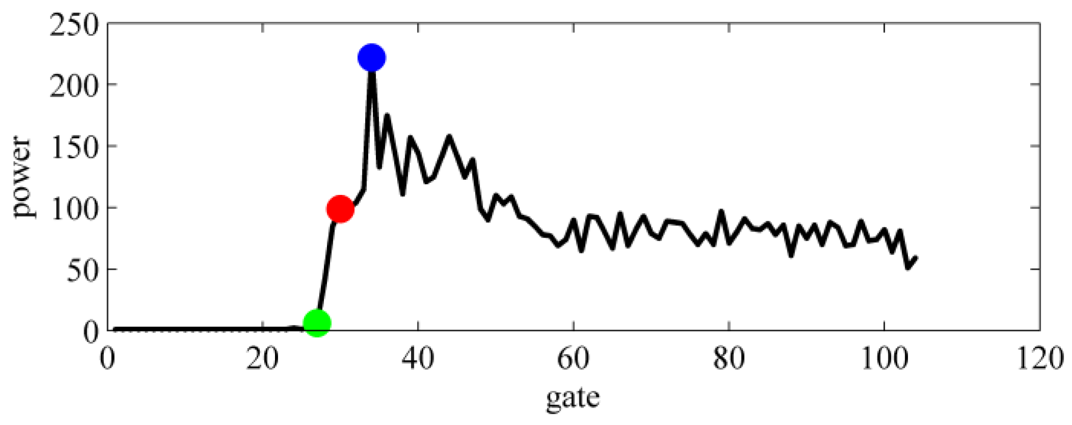
Figure 3, it is generally difficult to determine the SWH itself or the leading-edge length in an individual waveform. Moreover, as shown in 
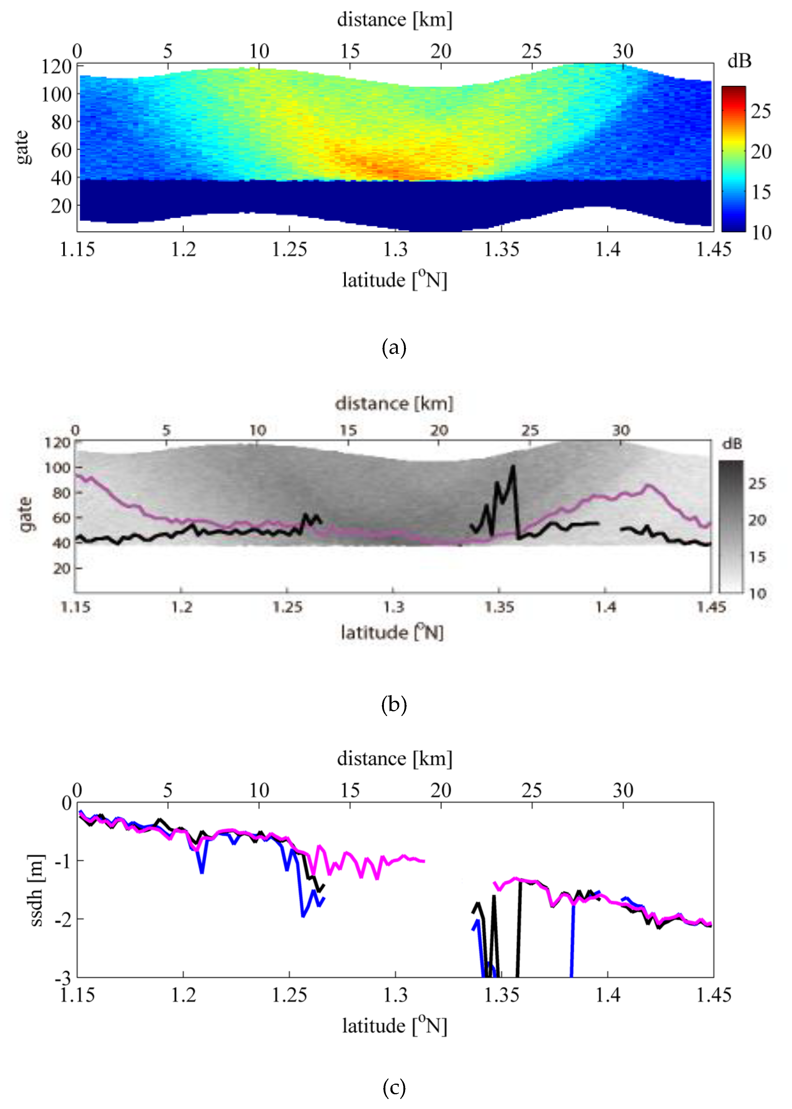
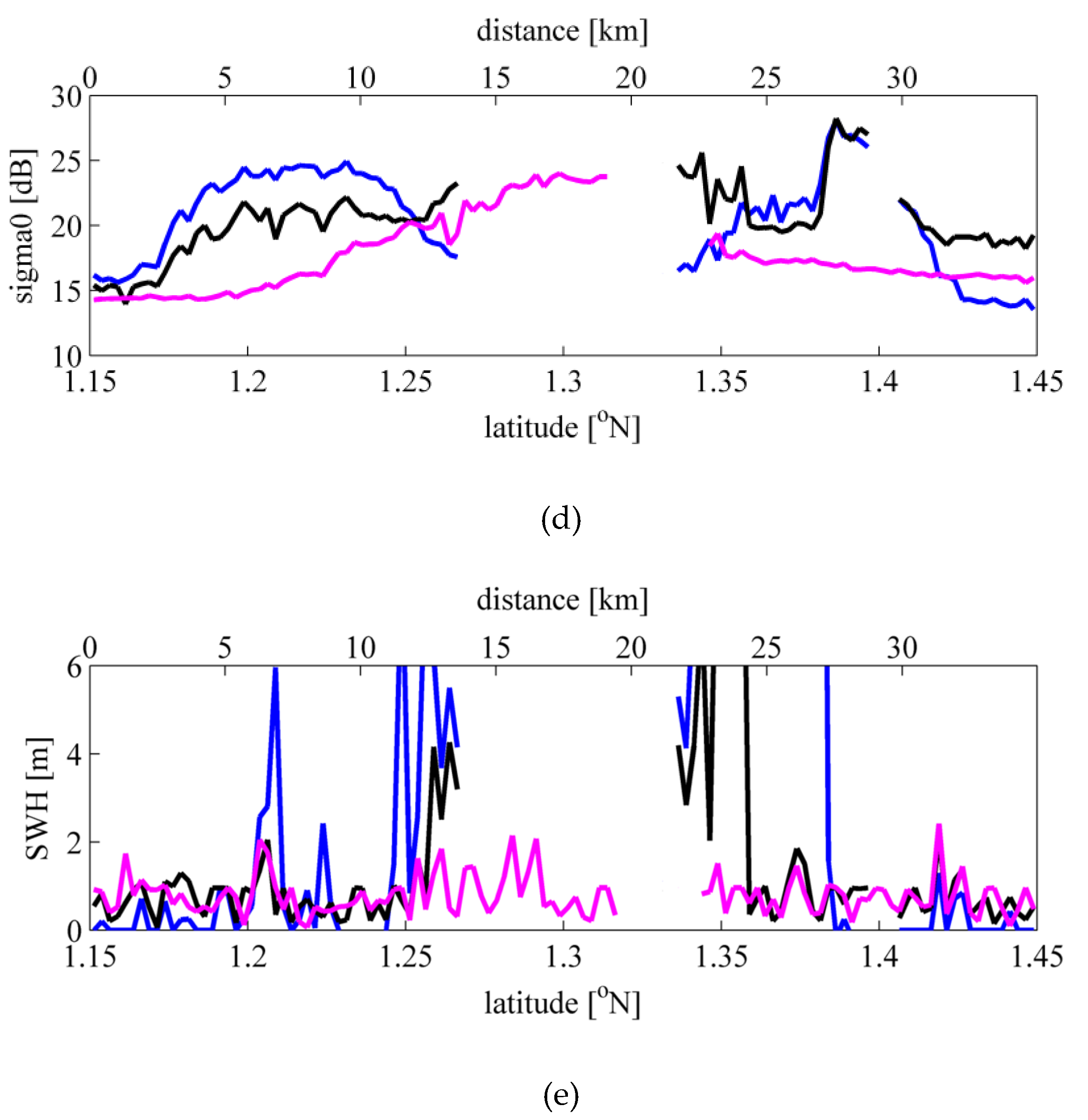
Figure 5, corrupted estimations of the trailing edge slope due to contaminated echoes from slicks could ruin the sigma0 and SWH estimates.
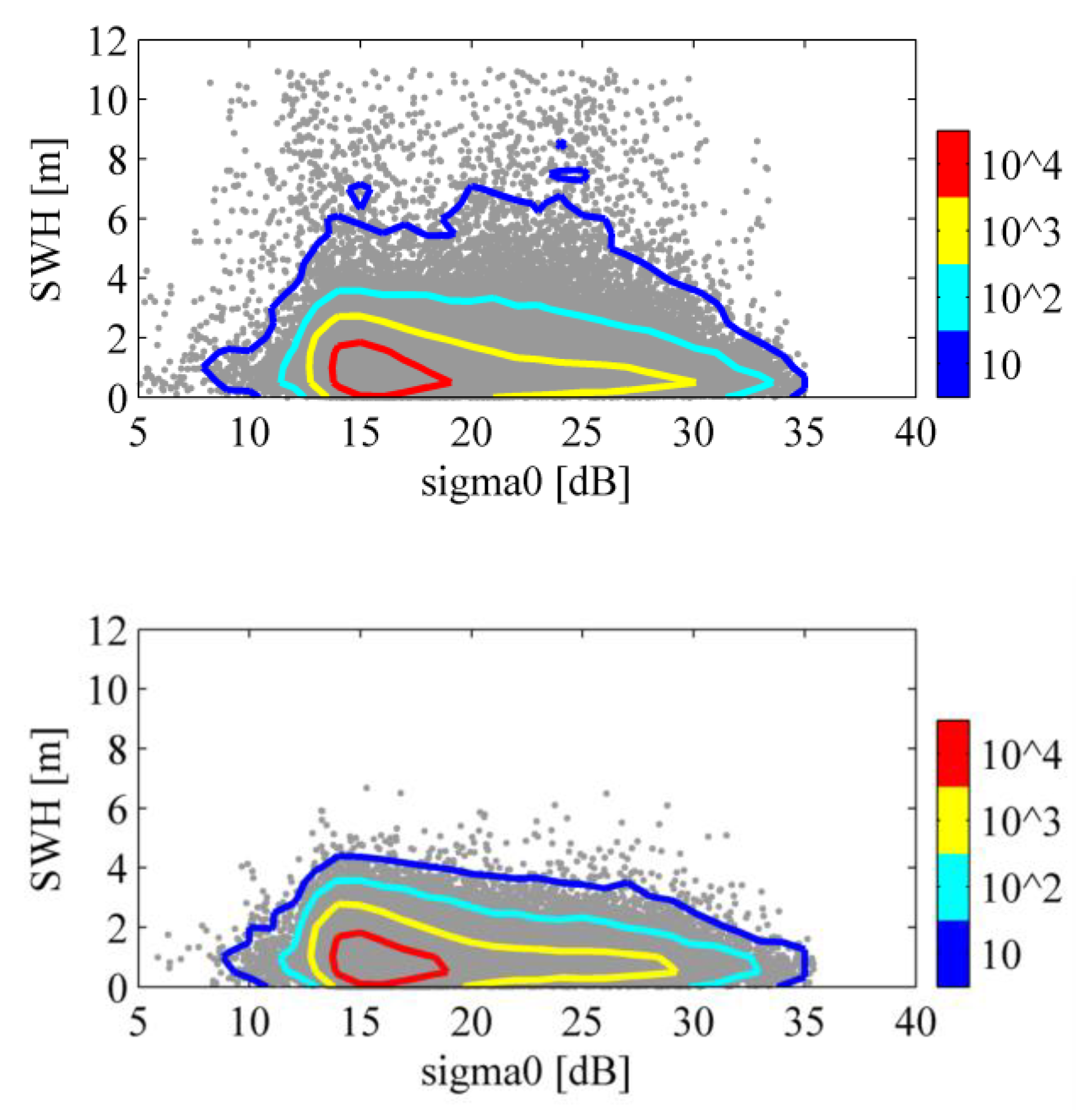
In order to evaluate the SWH and sigma0 estimates, scatter plots along Pass 101 are shown in Figure 11. Gray points represent the scatter points of SWH with sigma0 retrieved using the filtered ALES (top) and the present study (bottom). Note that the additional ALES data with sigma0 values from 5 to 7 dB and 30 to 35 dB were plotted for comparison. They are filtered by criteria in Table 1. The scatter plots are gridded with step sizes of 0.5 dB for sigma0 and 0.5 m for SWH, respectively, and the number of data points located within every grid point is shown using solid count lines in Figure 11. The contour lines are 10, 100, 1000, and 10,000 data numbers for each grid point.
In both datasets, data density distributions with more than 100 points were similar. The maximum data density was located at about 16 dB (sigma0) and 1 m (SWH), which were consistent with the weak wind and low wave height conditions typical in this region. In general, the contour lines show horizontally stretched oval shapes, suggesting smaller SWH values as sigma0 increases, i.e., with lower wind speeds. This tendency is consistent with the absence of significant swells, which is typical in semi-closed seas.
However, the contour lines with 10 data points behaved differently. In general, the ALES results were significantly scattered in the region of low data density. Unrealistically large SWH values of over 6 m were often found, although the data density in a grid was lower than 10. On the contrary, the contour line with 10 data points for the present study followed similar shapes to the other contour lines with larger data densities. Therefore, besides the SSDH results, the method proposed in the present study also improves sigma0 and SWH estimations.
In the present study, the length of the trailing edge was determined so that the echo intensity within the given footprint size did not significantly change in the echogram, i.e., integrated waveforms from the adjacent along-track points. A shorter trailing edge length indicates the presence of inhomogeneous sea surface roughness near the nadir, such as a case close to the edge of slicks. However, if the trailing edge length is too short, high-frequency noises in the trailing edge may not be removed properly in fitting of the Brown model. In other words, a criterion of the minimum length of the waveform trailing edge should be applied in the analysis to ensure reliable fitting of the Brown model.
In Table 3, statistics are listed for different criteria of the minimum trailing edge length. Together with the statistics listed in Table 2, the occurrence of the abnormal SWH is also counted in Table 3 as the cases where SWH exceeds 4 m even with low wind conditions (sigma0 is larger than 20 dB). In general, all four values decreased when the criterion became larger. The occurrence of abnormal SSDH estimations was most sensitive to changes of the criteria. In other words, the criterion of the minimum length of the trailing edge was a trade-off between the number of data points and the quality of the data. If the criterion is set as one gate, the data acquisition rate exceeds 99%, but abnormal SSHA values could be included although they were infrequent (approximately 100 times out of more than 480,000 occurrences). On the other hand, if the analysis is limited to a larger footprint size with more than 10 trailing edge gates, the abnormal SSHAs are rarely included, but the data acquisition rate decreases to nearly 80%. In the present study, three gates were provisionally used for the criterion of the minimum length of the trailing edge in order to obtain a similar data acquisition rate with the filtered ALES data, although the estimation accuracy would be less than when using larger criteria gates. Nevertheless, both the SSDH standard deviation and the occurrence of abnormal estimations were much better than the filtered ALES data (Table 2).
Note that the occurrence number of abnormal SWH estimations was less sensitive to changes of the criteria. Since the SWH was estimated form the length of the leading edge, the estimation error of the SWH would be large only when the trailing edge near the stop gate was contaminated. The difference of the stop gates between ALES and the present study is outlined in Figure 3. In a case when the red point is the true leading edge top, the peak of the blue point would be caused by contaminated echo from a slick near the nadir, which should produce a large error in the SWH estimation if included within the estimation window. Also note that the echo intensity in the trailing edge in Figure 3 is relatively large until gate 60, which would suggest that the influence of the possible slick is present between gates 32 and 60, and they would not be fully removed even if a long trailing edge is used.
The only way to remove these possible contaminations between gates 32 and 60 in Figure 3 is to limit the estimation window before the gate at the blue point. In the present study, the estimation window would be limited if the echo intensity at the blue point and/or surroundings in the echogram exceeded the practically determined threshold (3.5 dB). In other words, this threshold controls the sensitivity of the present method to slicks. At the same time, in order to smooth out noises in the trailing edge of the waveform, the threshold should not be too sensitive to the high-frequency noises of the waveforms. In the present study, the threshold value was practically determined as 3.5 dB by testing various values.

6. Summary

A new post-processed subwaveform retracking method is proposed in the present study, which uses variable footprint sizes with homogeneous sea surface roughness in order to hold proper fitting conditions of the Brown model. The echograms, or the integrated waveforms of the adjacent along-track observation points, were used to identify the subwaveform window size, which conquers uncertainty in the identification of contaminated echoes in a single waveform.
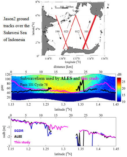
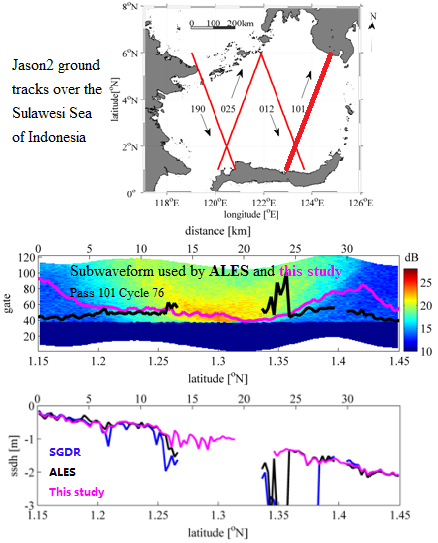
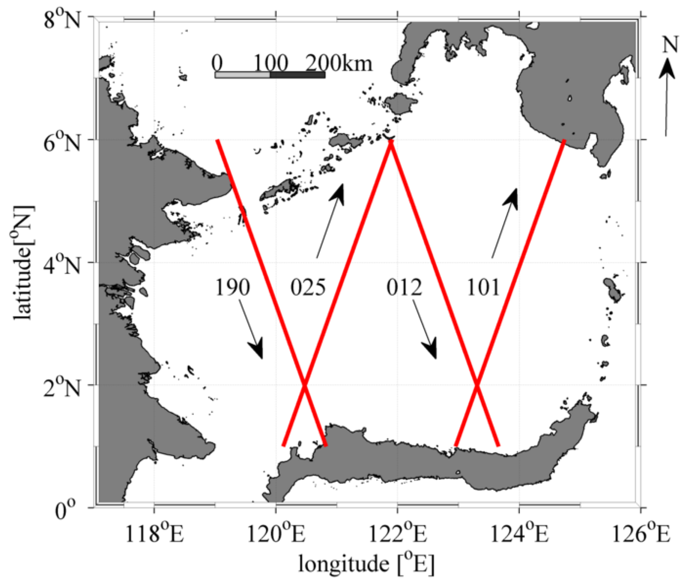
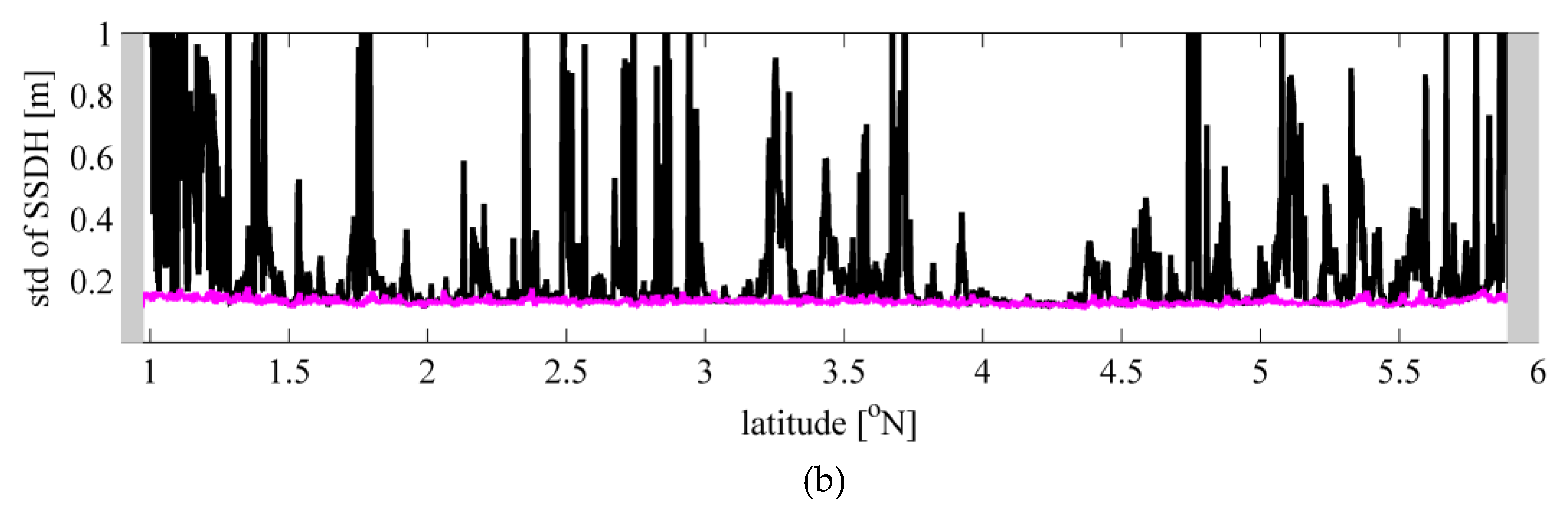
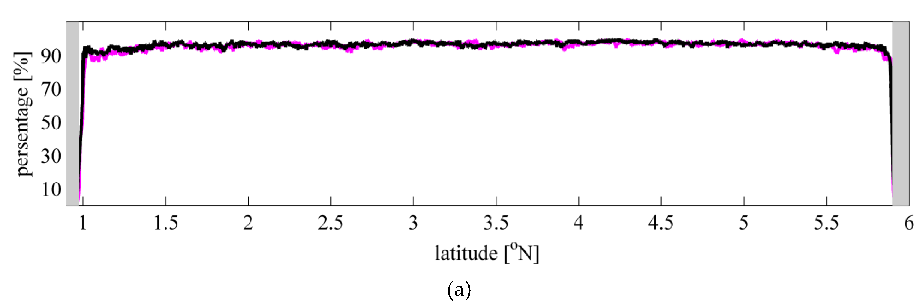
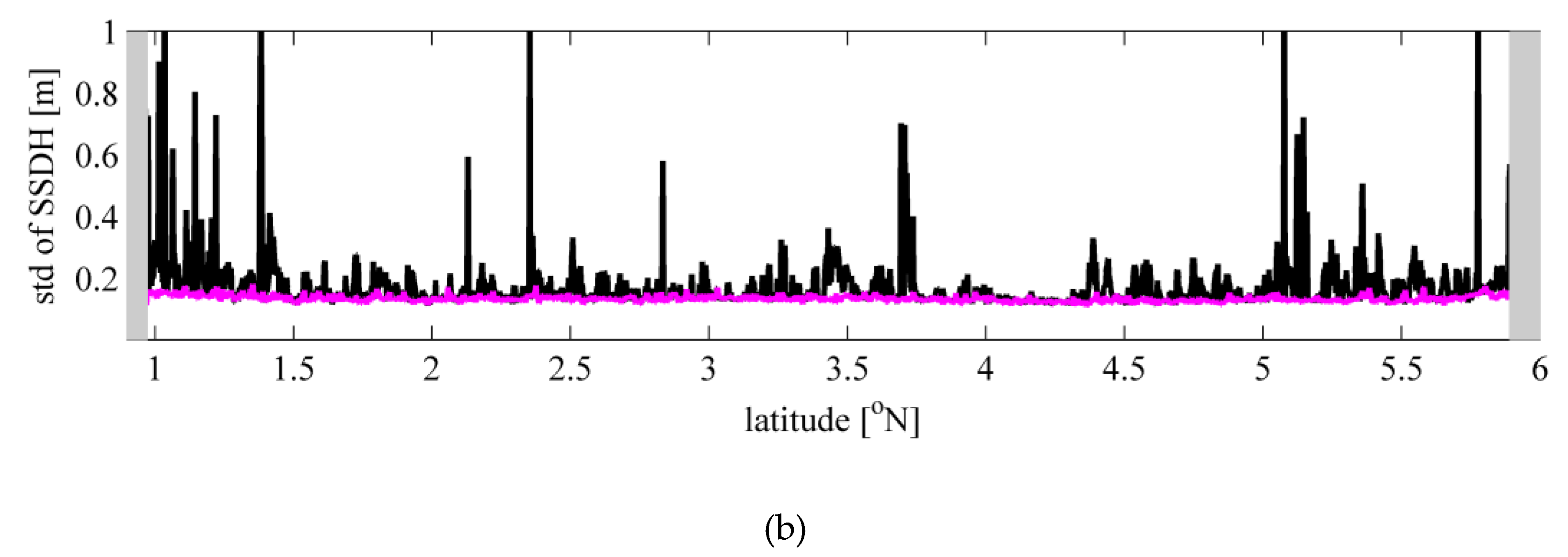
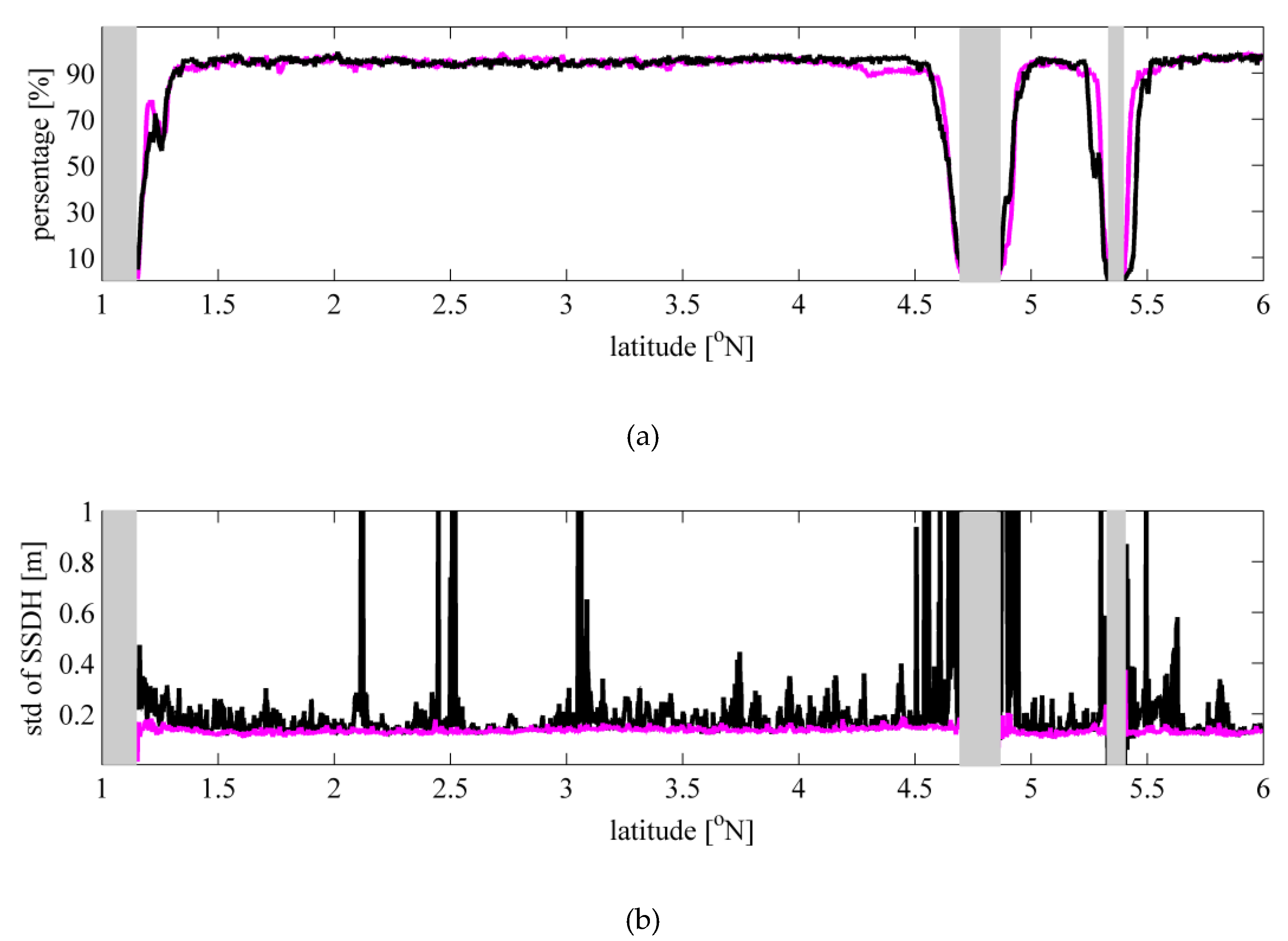
The 20 Hz Jason-2 altimeter data over the Sulawesi Sea of Indonesia was used for validation of our method, as slicks are often observed there. As shown in
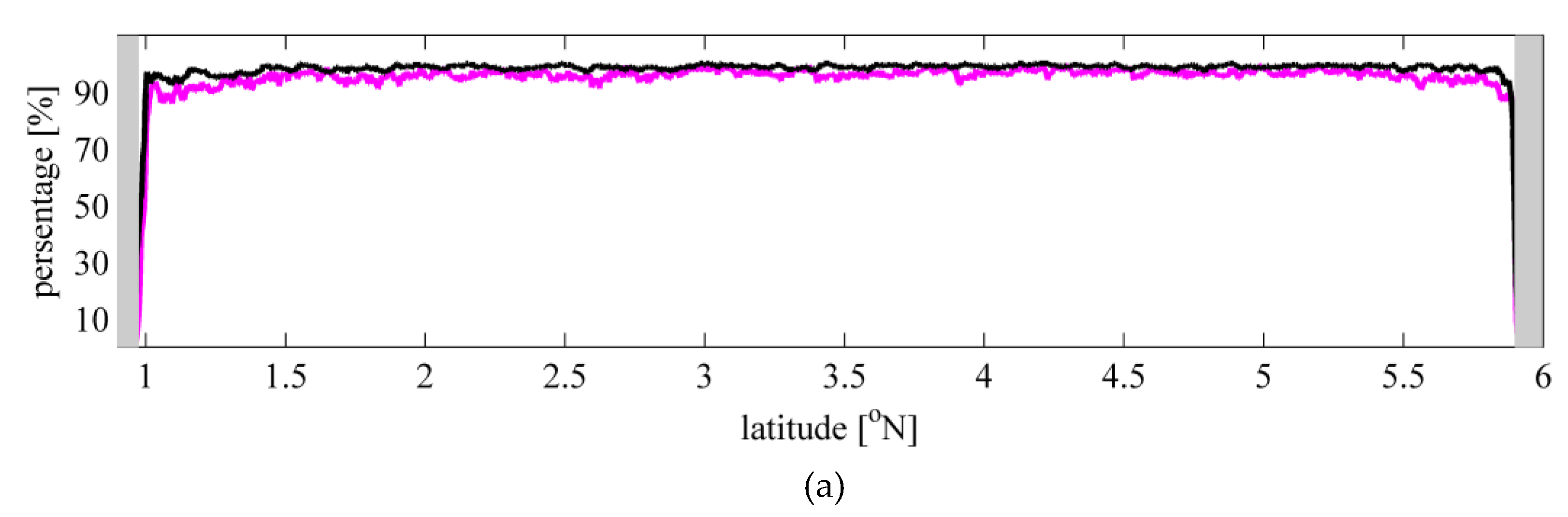
 Figure 7 and Figure 8, a data acquisition rate of more than 90% can be guaranteed approximately 5–10 km away from the coast, which is equivalent to that of the ALES data filtered by the conditions listed in Table 1. Meanwhile, the standard deviation of the SSDH of the present study is much smaller than that of the ALES results, not only in open seas but also in coastal waters. All the statistics in Table 2 indicates the advantages of the present method, especially because the occurrence number of abnormal SSDH values was 20 times smaller than that of ALES data and 200 times smaller than that of SGDR data.
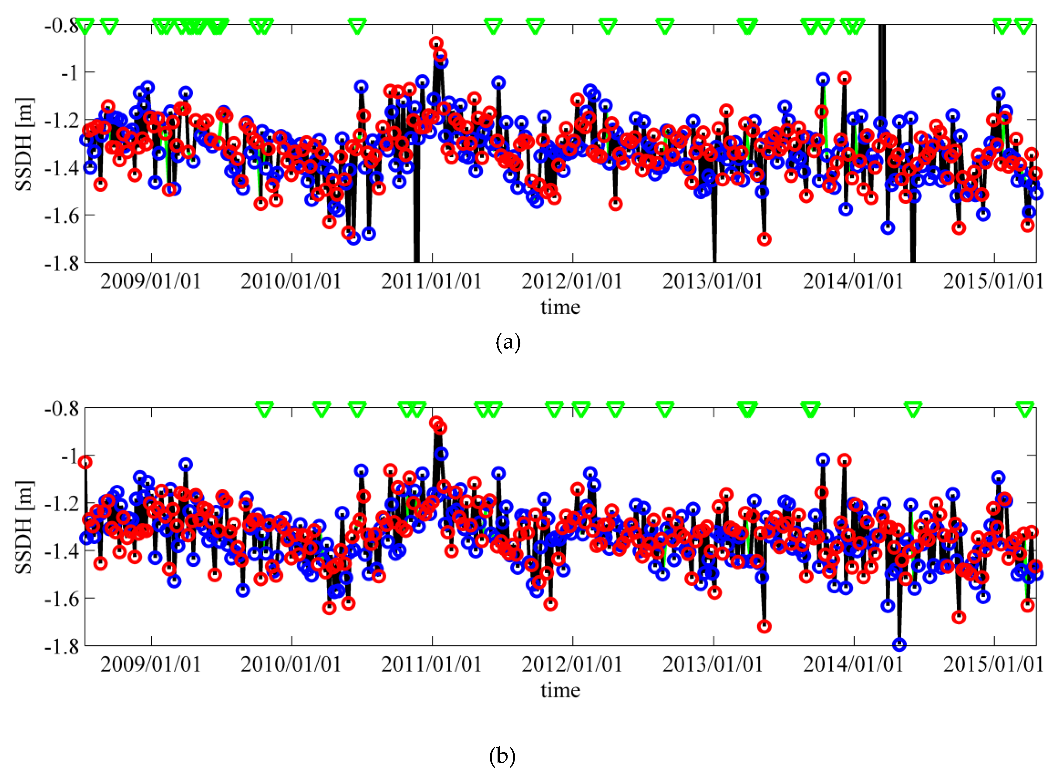
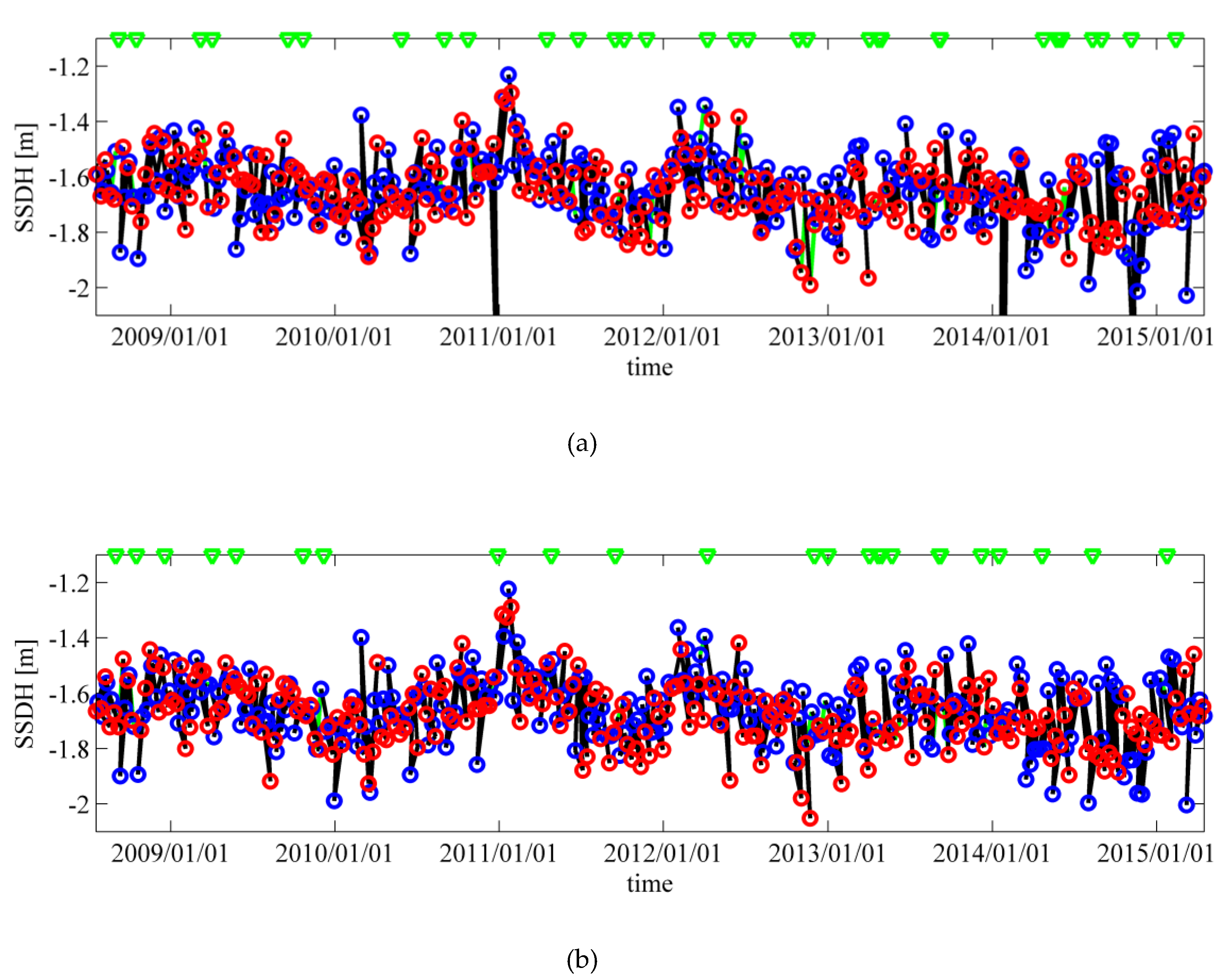
The time series of the SSDH were examined at the two crossover points of two passes (Passes 12 and 101; 190 and 25). Both ALES and the present study show similar smooth, long-term SSDH variations, but several outliers are included in the filtered ALES data. Since the SSDH standard deviation of the filtered ALES data is not significantly large at the crossover points, outliers would be more frequently observed in the ALES data at other points where its SSDH standard deviation is large. Note that the outlier-absent SSDH of the present study would be effective even in coastal areas where the ALES SSDH standard deviation is generally large.
The relationship between the sigma0 and SWH estimations was also examined along Pass 101 (Figure 11). The data density distributions of both ALES and this study indicate that SWH tends to be smaller when wind speed is low (i.e., sigma0 is large), which agrees with the conditions of the absence of significant swells that is typical in semi-closed seas. However, the ALES data shows significant scattering in a region with low data density. This suggests that the ALES occasionally failed in estimations of SWH or sigma0, probably due to contamination of echoes from slicks in the trailing edge slope.
Finally, dependency of the results on selections of the criteria parameters used in the present study, i.e., the minimum trailing edge length and the threshold value of homogeneous echo intensity, were examined. The minimum trailing edge length is a trade-off between the data acquisition rate and the quality of the data, while the threshold value is a trade-off between the sensitivity to echoes from slicks and that to noises in the trailing edge slope. Although they are practically determined in the present study by testing various values, these parameters could be set differently in other study areas and with different study targets. Further studies are required to generalize these requirements on the parameters.

Author Contributions

Data curation, X.W.; Methodology, K.I.; Resources, D.W.; Supervision, K.I.; Writing–original draft, X.W.

Acknowledgments

The present study was supported, in part, by The Japan Society for the Promotion of Science (JSPS) KAKENHI (Grant number JP15H05821). Marcello Passaro kindly provided the ALES data set for the Indonesian Seas.

Conflicts of Interest

The authors declare no conflict of interest.

References

  1. Brown, G. The average impulse response of a rough surface and its applications. IEEE Trans. Antennas Propag. 1977, 25, 67–74. [Google Scholar] [CrossRef]
  2. Hayne, G.S. Radar altimeter mean return waveforms from near-normal-incidence Ocean surface scattering. IEEE Trans. Antennas Propag. 1980, 28, 687–692. [Google Scholar] [CrossRef]
  3. Gommenginger, C.; Thibaut, P.; Fenoglio-Marc, L.; Quartly, G.; Deng, X.; Gomez-Enri, J.; Challenor, P.; Gao, Y. Retracking Altimeter Waveforms Near the Coasts. A Review of Retracking Methods and Some Applications to Coastal Waveforms. In Coastal Altimetry; Springer: Berlin, Germany, 2011; pp. 61–75. [Google Scholar]
  4. Gomez-Enri, J.; Vignudelli, S.; Quartly, G.D.; Gommenginger, C.P.; Cipollini, P.; Challenor, P.G.; Benveniste, J. Modeling Envisat RA-2 waveforms in the coastal zone: Case study of calm water contamination. IEEE J. Geosci. Remote Sens. Lett. 2010, 7, 474–478. [Google Scholar] [CrossRef]
  5. Tournadre, J. Signature of lighthouses, ships, and small islands in altimeter waveforms. J. Atmos. Ocean. Technol. 2007, 24, 1143–1149. [Google Scholar] [CrossRef]
  6. Thibaut, P.; Ferreira, F.; Femenias, P. Sigma0 blooms in the Envisat radar altimeter data. In Proceedings of the Envisat Symposium 2007, Montreux, Switzerland, 23–27 April 2007. [Google Scholar]
  7. Bao, L.; Lu, Y.; Wang, Y. Improved retracking algorithm for oceanic altimeter waveforms. Prog. Nat. Sci. 2009, 19, 195–203. [Google Scholar] [CrossRef]
  8. Idris, N.; Deng, X.L. The retracking technique on multi-peak and quasi-specular waveforms for Jason-1 and Jason-2 missions near the coast. Mar. Geod. 2012, 35, 217–237. [Google Scholar] [CrossRef]
  9. Passaro, M.; Cipollini, P.; Vignudeli, S.; Quartly, G.D.; Snaith, H.M. ALES: A multi-mission adaptive subwaveform retracter for coastal and open ocean altimetry. Remote Sens. Environ. 2014, 145, 173–189. [Google Scholar] [CrossRef]
  10. Wang, X.F.; Ichikawa, K. Coastal waveform retracking for Jason-2 altimeter data based on along-track echograms around the Tsushima islands in Japan. Remote Sens. 2017, 9, 762. [Google Scholar] [CrossRef]
  11. Tournadre, J. Determination of rain cell characteristics from the analysis of TOPEX altimeter echo waveforms. J. Atmos. Ocean. Technol. 1998, 15, 387–406. [Google Scholar] [CrossRef]
  12. OSTM/Jason-2 Products Handbook; Le site du Centre national d’études spatiales (CNES): Paris, France, 2015.
Figure 1. Ground tracks (red lines) of the Jason-2 altimeter over the Sulawesi Sea of Indonesia. The numbers and arrows indicate the pass number and the direction of the satellite, respectively.
Remotesensing 11 01274 g001
Figure 2. (a) Circular slick with a radius of 5 km located in the altimeter nadir track. (b) V-shaped pattern of echoes from the circular slick in the echogram of the Jason-2 altimeter. The color scale is in arbitrary units.
Remotesensing 11 01274 g002
Figure 3. Example of the difference in the leading edges detected by the adaptive leading edge subwaveform retracker (ALES) and in the present study (Pass 101, Cycle 011, at 2.1203° N latitude). The green point is the common edge foot of the two methods. The red point is the edge top of the present study. The blue point is the edge top of ALES.
Remotesensing 11 01274 g003
Figure 4. Overview of the determination of the estimation window. (a) Altimeter footprint. (b) The enhanced triangular intersections in the echogram. Gates G1 and G2 correspond to different footprint sizes.
Remotesensing 11 01274 g004
Figure 5. Example of a strong relative brightness slick (Pass 101, Cycle 76). (a) Echogram. The power is corrected for antenna attenuation and the waveforms are realigned as described in Section 3.2. (b) Estimation window of two subwaveform retrackers. (c) Retrieved sea surface dynamic height (SSDH) of three retrackers. (d) Retrieved sigma0 of three retrackers. (e) Retrieved significant wave height (SWH) of three retrackers. Blue lines: sensor geophysical data record (SGDR); Black lines: ALES; Purple lines: the present study.
Remotesensing 11 01274 g005aRemotesensing 11 01274 g005b
Figure 6. (a) Comparison of the data acquisition rate and (b) the standard deviation of SSDH along Pass 101 between original ALES (black) data and the present study (purple). The shaded areas (gray patches) correspond to land.
Remotesensing 11 01274 g006aRemotesensing 11 01274 g006b
Figure 7. (a) Comparison of the data acquisition rate and (b) the standard deviation of SSDH along Pass 101 between the filtered ALES data (black) and the present study (purple). The shaded areas (gray patches) correspond to land.
Remotesensing 11 01274 g007aRemotesensing 11 01274 g007b
Figure 8. (a) Comparison of the data acquisition rate and (b) the standard deviation of SSDH along Pass 190 between the filtered ALES data (black) and the present study (purple). The shaded areas (gray patches) correspond to land.
Remotesensing 11 01274 g008
Figure 9. (a) Time series of the SSDH at the crossover point of Passes 012 and 101 (see Figure 1) of the filtered ALES data. (b) Time series of the SSDH at the crossover point of Passes 012 and 101 of the present study. Red and blue circles represent the SSDH of Pass 012 and 101, respectively. Data are connected by black lines if there are no missing data, otherwise they are connected by green lines. The green triangles in the two figures indicate the location of SSDH gaps.
Remotesensing 11 01274 g009
Figure 10. (a) Time series of the SSDH at the crossover point of Passes 190 and 025 (see Figure 1) of the filtered ALES data. (b) Time series of the SSDH at the crossover point of Passes 190 and 025 of the present study. Red and blue circles represent the SSDH of Pass 190 or 025, respectively. Data are connected by black lines if there are no missing data, otherwise they are connected by green lines. The green triangles in the two figures indicate the location of SSDH gaps.
Remotesensing 11 01274 g010
Figure 11. Scatter plots of sigma0 with SWH retrieved using (a) filtered ALES and (b) the present study along Pass 101. Solid lines represent the contours of the data number in each 0.5-dB and 0.5-m grid. Note that the ALES results were filtered using the criteria listed in Table 1, but the data with sigma0 values varying from 5 to 35 dB were retained for comparison.
Remotesensing 11 01274 g011
Table 1. Filtering criteria for ALES data used in the present study.
ParameterValidity Conditions
MQE (ALES)
MQE (SGDR)
0 ≤ x (count) ≤ 0.15
0 ≤ x (count) ≤ 0.30
SSH (ALES and SGDR)−130 ≤ x (m) ≤ 100
SWH (ALES and SGDR)0 ≤ x (m) ≤ 11
Sigma0 (ALES and SGDR)7 ≤ x (dB) ≤ 30
Table 2. Statistical comparisons of the data acquisition rate and the SSDH standard deviation in ALES and SGDR products.
Pass NumberProductFiltering CriteriaMean Data Acquisition Rate (%)Mean Standard Deviation (m)Number of Abnormal Value Occurrences (SSDH)
012
250 cycles
1−6° N
This studyThree gates95.50.12851
ALESOriginal98.50.2541633
Filtered 95.60.1691134
SGDROriginal99.70.62020,066
Filtered96.60.49114,435
025
250 cycles
1−6° N
This studyThree gates96.00.13160
ALESOriginal98.70.2411548
Filtered95.80.1701112
SGDROriginal99.80.64421,599
Filtered97.70.52516,788
101
250 cycles
1−6° N
This studyThree gates97.10.12941
ALESOriginal98.50.2581777
Filtered96.30.16711,88
SGDROriginal99.70.62417,895
Filtered97.10.49912,008
190
250 cycles
1−6° N
This studyThree gates89.00.13363
ALESOriginal92.10.80012,310
Filtered88.50.2241769
SGDROriginal93.10.94444,438
Filtered87.80.76322,145
Table 3. Statistical comparison of data acquisition rate, standard deviation, and number of abnormal values using different minimum lengths of the trailing edge.
Pass NumberMinimum Trailing Edge LengthMean Data Acquisition Rate (%)Mean Standard Deviation (m)Number of Abnormal Value Occurrences (SSDH)Number of Abnormal Value Occurrences (SWH)
012
250 cycles
1–6° N
1 gate99.10.13110183
3 gates95.50.1285167
5 gates93.10.1263239
7 gates87.00.1241225
10 gates80.90.122620
025
250 cycles
1–6° N
1 gate97.80.1338381
3 gates96.00.1316069
5 gates91.80.1293247
7 gates88.70.1282433
10 gates81.00.1261526
101
250 cycles
1–6° N
1 gate99.20.1329372
3 gates97.10.1294256
5 gates93.40.1272039
7 gates87.40.124733
10 gates82.80.123328
190
250 cycles
1–6° N
1 gate92.10.13712761
3 gates89.00.1336350
5 gates83.40.1292928
7 gates79.70.1271818
10 gates71.20.125516

