GOCE-Derived Coseismic Gravity Gradient Changes Caused by the 2011 Tohoku-Oki Earthquake


1
School of Geodesy and Geomatics, Wuhan University, Wuhan 430079, China
2
State Key Laboratory of Information Engineering in Surveying, Mapping and Remote Sensing, Wuhan University, Wuhan 430079, China
3
Shanghai Astronomical Observatory, Chinese Academy of Sciences, Shanghai 200030, China
4
Key Laboratory of Earthquake Geodesy, Institute of Seismology, China Earthquake Administration, 40 Hongshan Celu, Wuhan 430071, China
*
Author to whom correspondence should be addressed.
Remote Sens. 2019, 11(11), 1295; https://doi.org/10.3390/rs11111295
Submission received: 11 April 2019
/
Revised: 25 May 2019
/
Accepted: 25 May 2019
/
Published: 30 May 2019
(This article belongs to the Special Issue Remote Sensing by Satellite Gravimetry)
Abstract
:In contrast to most of the coseismic gravity change studies, which are generally based on data from the Gravity field Recovery and Climate Experiment (GRACE) satellite mission, we use observations from the Gravity field and steady-state Ocean Circulation Explorer (GOCE) Satellite Gravity Gradient (SGG) mission to estimate the coseismic gravity and gravity gradient changes caused by the 2011 Tohoku-Oki Mw 9.0 earthquake. We first construct two global gravity field models up to degree and order 220, before and after the earthquake, based on the least-squares method, with a bandpass Auto Regression Moving Average (ARMA) filter applied to the SGG data along the orbit. In addition, to reduce the influences of colored noise in the SGG data and the polar gap problem on the recovered model, we propose a tailored spherical harmonic (TSH) approach, which only uses the spherical harmonic (SH) coefficients with the degree range 30–95 to compute the coseismic gravity changes in the spatial domain. Then, both the results from the GOCE observations and the GRACE temporal gravity field models (with the same TSH degrees and orders) are simultaneously compared with the forward-modeled signals that are estimated based on the fault slip model of the earthquake event. Although there are considerable misfits between GOCE-derived and modeled gravity gradient changes (ΔVxx, ΔVyy, ΔVzz, and ΔVxz), we find analogous spatial patterns and a significant change (greater than 3σ) in gravity gradients before and after the earthquake. Moreover, we estimate the radial gravity gradient changes from the GOCE-derived monthly time-variable gravity field models before and after the earthquake, whose amplitudes are at a level over three times that of their corresponding uncertainties, and are thus significant. Additionally, the results show that the recovered coseismic gravity signals in the west-to-east direction from GOCE are closer to the modeled signals than those from GRACE in the TSH degree range 30–95. This indicates that the GOCE-derived gravity models might be used as additional observations to infer/explain some time-variable geophysical signals of interest.
1. Introduction
Because satellite gravity observations are not limited to Earth’s surface conditions, and can cover the whole Earth quickly, they provide an independent way to detect the coseismic effects of large earthquakes, which is a good complement for other earthquake measurements (e.g., surface deformations), and are of great scientific significance.
A new generation of satellite gravimetry missions, including CHAMP (CHAllenging Minisatellite Payload) [1], GRACE (Gravity field Recovery and Climate Experiment) [2] and GOCE (Gravity field and steady state Ocean Circulation Explorer) [3], have been successfully implemented to detect global static and time-variable gravity signals. A large number of real observations and derived products from the CHAMP, GRACE and GOCE missions have been applied to Earth-science research, especially temporal gravity signals derived from the GRACE mission, which are used to monitor mass transport in the Earth system. The detection of coseismic gravity change signals using GRACE data has been widely studied. Generally, monthly gravity field models from GRACE before and after the earthquake were used to derive coseismic gravity or gravity gradient changes. Long-to-medium-wavelength coseismic and post-seismic gravity changes from large-scale earthquakes (e.g., the 2004 Sumatra-Andaman Mw = 9.1, 2010 Maule Mw = 8.8, 2011 Tohoku-Oki Mw = 9.0) have been adequately detected by the GRACE mission [4,5,6,7,8,9,10,11,12,13,14,15,16,17]. Wang et al. [13] and Li and Shen [17] also determined the coseismic gravity gradient changes caused by the 2011 Japan Tohoku-Oki earthquake. The GOCE mission has been proven successful for constructing regional geoid models combining with the EGM2008 and terrestrial gravity datasets [18,19], and can be used to study the lithospheric modeling, dynamic topography, and glacial isostatic adjustment [20,21,22,23]. However, a few studies have focused on inferring the coseismic gravity change signals from simulated data [24,25,26] or real GOCE observations [27,28,29].
The main scientific objective of the GOCE mission is to recover static gravity field models up to degree and order (d/o) 200 by using SGG (Satellite Gravity Gradient) observations [3]. Because of the lower sensitivity of the gradiometer on board of the GOCE satellite at lower frequencies, the gravity gradient observations are not sensitive to temporal signals, the main power of which is at long wavelengths (commonly, at spatial resolutions higher than 1500 km) [30,31]. However, the coseismic gravity change signals from the 2011 Japan Tohoku-Oki earthquake were still detected by the GOCE mission [27,28]. Garcia et al. [27] showed that GOCE’s gradiometer, acting similarly to a seismometer in orbit, recorded the sound waves from the 2011 Tohoku earthquake. Fuchs et al. [28] combined a new vertical gravity gradient from the diagonal components (Vxx, Vyy, and Vzz) along the orbit. The coseismic radial gravity gradient changes ΔVzz in Fuchs et al. [28] were derived by subtracting the vertical gravity gradients computed by a reference model GOCO03s [32] from with an along track and spatial filter applied to deal with the colored noise. Fuchs et al. [28] mentioned that they did not use the spatiospectral localization method like Han and Ditmar [26] to process geopotential coefficients, because there were no released global gravity field models (GGMs) from the post-earthquake GOCE data that could be used to detect coseismic gravity gradient changes.
In this paper, we choose a different approach than that proposed in Fuchs et al. [28]. First, we recover the GGMs (SH coefficients) before and after the earthquake from GOCE gravity gradient observations (Vxx, Vyy, and Vzz) along the orbit, based on the least-squares method. Note that, Fuchs et al. [28] did not estimate the SH coefficients of the pre- and post-earthquake global time-variable gravity field models. Then, we estimate the gravity changes (Δg) and the gravity gradient changes (ΔVxx, ΔVyy, ΔVzz, and ΔVxz) from the differences between two recovered global gravity models. In order to weaken the influences of colored noise and the polar gap problem from GOCE SGG observations on the recovered model, we use a tailored spherical harmonic (TSH) coefficients to recover the coseismic gravity change. Finally, we compare the results obtained from forward-modeled signals with the GRACE monthly gravity field models. Compared to Fuchs et al. [28], our approach can determine the coseismic gravity changes and the coseismic gravity gradient changes of other gravity gradient tensor (GGT) components in addition to ΔVzz. The content of this manuscript is organized into four sections, beginning with a description of the methodology of GOCE data processing, forward modeling coseismic gravity gradient changes, and the computation of TSH coefficients in Section 2. The results and analysis are presented in Section 3. A summary and concluding remarks are provided in Section 4.
2. Methodology
2.1. Recovering Gravity Field Model from GOCE SGG Observations
In this paper, we derive the coseismic gravity and gravity gradient changes by evaluating the differences between a post-earthquake gravity field model and a pre-earthquake one from GOCE data; namely, we first recover gravity field models from the Gravity field and steady state Ocean Circulation Explorer Satellite Gravity Gradient (GOCE SGG) observations before and after the 2011 Tohoku-Oki earthquake. Here, we provide a brief description of the data processing strategies of recovering a gravity field model from GOCE SGG observations (more details can be found in Xu et al. [33]).
The component Vij of the second-order gravity gradient tensor (GGT) is normally defined in the Local North-Oriented Frame (LNOF) with the x-axis pointing north, the y-axis pointing west and the z-axis up, as follows [33]:
where the indices i and j define the gravitational gradient components (xx, yy, zz, xy,…) with respect to the LNOF axes (x, y, z); the indices n and m are the degree and order, respectively, of the spherical expansion; and are the spherical coordinates in the Earth’s Fixed Reference Frame (EFRF), where r is the geocentric radius; and θ and λ are the spherical colatitude and longitude, respectively. and are the (fully normalized) geopotential cosine and sine coefficients. and are the Fourier coefficients and transform coefficients, respectively; for more details, please refer to Koop [34].
Based on Equation (1), the functional and statistical models of the gravitational field recovered from the Satellite Gravity Gradient (SGG) data are defined as a standard Gauss-Markov model. Then, we can determine the geopotential coefficients and , exploiting the least-squares (LS) method. However, the observed GGT of the GOCE mission is given in the Gradiometer Reference Frame (GRF), so we should transform the observations from the GRF to the LNOF by using the rotation matrix [33]. However, the accuracies of the Vxy and Vyz components are lower than those of the other components, so they will contaminate the high-precision components (Vxx, Vyy, Vzz, and Vxz) in the transformation. To avoid this situation, we transform the base functions () in Equation (1) instead of transforming the GGT observations in GRF. In particular, we multiply the matrix and its transposed matrix on both sides of the base functions in Equation (1) at every epoch. Hence, we have
where VGRF and VLNOF represent the gravitational gradient tensor in the GRF and LNOF, respectively.
Because the power spectral density (PSD) of the trace of the GGT represents the total error of the summation of the diagonal components (Vxx, Vyy, Vzz), the SGG observations are high-precision only within the designed measurement bandwidths (MBW) from 0.005 to 0.1 Hz according to Figure 1 [35]. The noise outside of this MBW increases with the decreasing frequency for frequencies below 0.005 Hz, and the increasing frequency for frequencies above 0.1 Hz, especially for the 1/f behavior at low frequencies, which show the character of the colored noise of the gradiometer [35]. To handle this colored noise in the SGG data, we apply a bandpass Auto Regression Moving Average (ARMA) filter with a pass-band of 0.005–0.041 Hz to both sides of the linear observation equation, these being Equation (2) and Equation (1) [36]. The maximum frequency (0.041 Hz) of the pass-band approximately corresponds to the maximum degree (220) of the recovered gravitational potential model based on the following formula:
where Tr = 5383 s is one satellite orbital revolution (cf. [37]).
According to Figure 1, the noise level of the components Vxx and Vyy is about 10 mE/ (1 mew = 10−12/s−2), that of Vzz is about 20 mE/, which is consistent with Rummel et al. [38]. Thus, to combine the diagonal components (Vxx, Vyy, and Vzz) in the LS, we set the ratio of the standard deviation factors of Vxx, Vyy, and Vzz to 1:1:2.
2.2. Tailored Spherical Harmonic Coefficients
Based on the data processing strategies in Section 2.1, the post-earthquake and pre-earthquake gravity field models can be recovered from GOCE SGG data. However, the lower and higher frequency bands of the recovered models are heavily influenced by the 0.005–0.041 Hz band-pass ARMA filter. Moreover, the polar gap problem of GOCE’s orbit mainly affects the low-order spherical harmonic (SH) coefficients. We perform a numerical simulation to show how the recovered model’s SH coefficients are affected by the band-pass filter and the polar gap problem. First, a 1 s sampling of 61-day GOCE satellite orbits are produced from the released reduced-dynamic orbit data (SST_PRD_2), with 10 s sampling by polynomial interpolation. Then, we simulate the GGT observations along the orbit by using the EGM2008 model up to d/o 220. We add simulated colored noise according to the prior PSD of the GGT’s trace, as given by Cesare [35], to the simulated GGT data. Finally, by using these simulated observations, we recover the gravity field model based on the LS approach with the 0.005–0.041 Hz band-pass filter applied. The absolute errors of the recovered model’s SH coefficients are obtained by calculating the difference between the model and the EGM2008 model. Figure 2 displays the error spectra of SH coefficients in log10 scale. According to this figure, SH coefficients up to d/o 160 with large errors are mainly located in the arrow-shaped region, which is framed by the red lines. Referring to the conclusions by Sneeuw [39], the errors of the near-zonal coefficients (m ≤ 10) are mainly caused by the ill-posed problem occasioned by the 96.7° inclination of the GOCE satellite orbit. The other coefficients with large errors in the arrow-shaped region are due to the lower frequency limit of the band-pass filter. The coefficients outside the arrow region are called the tailored spherical harmonic (TSH) coefficients here, which correspond to two symmetrical quadrilaterals. These TSH coefficients will be used to show the coseismic gravity and gravity gradient changes.
As shown in Figure 2, the degree of the middle corner coefficients in the arrow-shaped region is approximately 30, which is very close to the degree 27 estimated by Equation (3), according to the minimum frequency of the 0.005–0.041 Hz band-pass filter. Thus, the minimum degree of the TSH coefficients is set to 30 herein. The vertices of the lower-left and lower-right corners of the arrow region approximately correspond to a degree of 80. Fuchs et al. [28] presented their results according to three bandwidths (0.005–0.05, 0.0039–0.03, and 0.00475–0.0175 Hz), and the bandwidth of 0.00475–0.0175 Hz was determined by the matched filter approach, which maximizes the expected signal. The degree range 30–95 approximately corresponds to the bandwidth of 0.005–0.0175 Hz [28]. So, we also choose 95 (see the red dashed line in Figure 2) for the maximum degree of the TSH coefficients. Moreover, the maximum degree of 95 is very close to the maximum d/o of the SH coefficients of Gravity field Recovery and Climate Experiment (GRACE)’s time-variable gravity field model, so we can compare the results from GRACE with those from GOCE at the same frequency band.
2.3. Post-earthquake Gravity Changes from GOCE
Based on the theory and data processing strategies described above, we estimated two GGMs (the pre-earthquake model and the post-earthquake model) up to d/o 220 from the released GOCE’s calibrated and corrected gravity gradients in the GRF (EGG_NOM_2 products) (GGT and IAQ) and precise science orbits with quality report (SST_PSO_2 products) (PRD and PRM) [40] before and after the 2011 Japan Tohoku-Oki earthquake. The IAQ products are the GRF to IRF attitude quaternions, and the PRM products are the Earth Fixed Reference Frame (EFRF) to Inertial Reference Frame (IRF) quaternions. We selected the data period from the 1st of November 2009 until the 28th of February 2011 for the pre-earthquake time span, and the period from the 15th of March 2011 until the 31st of May 2012 for the post-earthquake time span. Only the high-precision diagonal components (Vxx, Vyy, and Vzz) of the GGT are selected for modeling. Before forming the observation equation, some data preprocessing tasks were performed, such as data interpolation and outlier detection [33]. For a more detailed description of GGT data processing, please refer to Xu et al. [33]. To reduce the influence of high-frequency errors, a Gaussian filter with the smoothing radius of 210 km is also applied to the TSH coefficients. A radius of 210 km for the Gaussian filter is approximately determined with the formula 20000 km/Nmax, corresponding to a maximum degree Nmax of 95.
2.4. Post-earthquake Gravity Changes from GRACE
For comparison with GOCE, we also derived the coseismic gravity changes and gravity gradient changes from the Release05 (RL05) GRACE time-variable monthly gravity field models from the Center for Space Research (CSR), which were downloaded from the website http://icgem.gfz-potsdam.de/ICGEM/. The maximum d/o was 96.
The TSH coefficients that corresponded to the SH degree range 30–95 were chosen to maintain consistency with the processing of the GOCE models, and a Gaussian filter with the smoothing radius of 210 km was also applied to the TSH coefficients. The differences in the coefficients between the averages of the monthly models for one year before and after the earthquake were used to calculate the coseismic gravity changes and gravity gradient changes on a sphere with a height of 260 km.
2.5. Forward Modeling Coseismic Gravity and Gravity Gradient Changes
The PSGRN/PSCMP code for the modeling co- and post-seismic response of the Earth’s crust to earthquakes from Wang et al. [41] is used to compute the coseismic gravity changes of the 2011 Tohoku-Oki earthquake based on a five-layer half-space Earth model and the fault slip model from Caltech provided by Wei and Sladen [42]. The layer depths, densities, and seismic velocities are extracted from the CRUST2.0 global tomography model [43], which are derived from the epicenter (38.1°N, 142.8°E) grid cell layer parameters, and are shown in Table 1. The upper four crustal layers in the model are treated as elastic materials. The bottom half-space mantle layer is treated as biviscous materials, i.e., a Burgers body with a transient (Kelvin) viscosity and a steady state (Maxwell) viscosity (Details about the Burgers viscosities will be described in Section 2.6). The free-air corrections, as calculated by the vertical surface displacements, are added to the calculated coseismic gravity changes from the PSGRN/PSCMP program [9]. A Bouguer layer seawater compensation effect is also corrected according to the vertical displacements with the consideration of the land-ocean differentiation [44]. Since Broerse et al. [44] pointed out that simply considering a global ocean for the seawater correction would lead to non-negligible errors (up to a few 10% for the 2011 Tohoku-Oki earthquake), using a practical land-ocean mask ensures a more reliable seawater effect correction for the model prediction in our study.
The computation region is from 28°N to 48°N latitude and from 132°E to 152°E longitude. The epicenter (38.1°N, 142.8°E) is located at the center of this region. The cell size of the grid is set to 0.1° × 0.1°. The global gridded coseismic gravity changes on a sphere are formed by the forward-modeled coseismic gravity changes, as well as filling in zero values outside the computational region. Based on the global gridded coseismic gravity changes, we estimate the gravitational potential spherical harmonic (SH) coefficients up to d/o 250, by using the classical spherical harmonic analysis approach [45]. Then, based on the estimated gravitational potential SH coefficients, we calculate changes of both the coseismic gravity and radial gravity gradient on the Earth’s surface and on a sphere with a height of 260 km above the WGS84 reference ellipsoid, which are shown in Figure 3 and Figure 4. According to the maximum d/o 250 of the SH coefficients, we use a Gaussian filter with a radius of 110 km here. The epicenter is also shown as a black star in these figures. The units of the gravity and the gravity gradient are mGal (1 mGal = 10−5 ms−2) and mE, respectively. According to Figure 3 and Figure 4, the spatial patterns of the coseismic gravity changes and gravity gradient changes show classic dipole characteristics in the nearly west-to-east direction. Additionally, the attenuation effect of the coseismic gravity change signal at the satellite height is very clear.
The amplitudes of the coseismic gravity changes and coseismic radial gravity gradient changes are reduced by more than a factor of 10 and 20, respectively.
2.6. Modeling of Post-seismic Gravity Changes
For the GOCE and GRACE observations, the coseismic gravity field changes are estimated by using the differences in coefficients between the pre-earthquake model and the post-earthquake model. Here we note that taking the one-year mean field differences as the coseismic signals will inevitably bring in the impact of the post-seismic effects, which are likely to affect the peak-to-peak range, as well as the spatial pattern of the extracted signals [46]. Han et al. [46] revealed that a dominant post-seismic positive gravity change signal is visible surrounding the epicenter within a couple of years after the 2011 Tohoku-Oki earthquake, with the amplitude up to around +6 μGal under a 500 km spatial scale comparable as GRACE observations. Moreover, they gave the results from aviscoelastic relaxation model and an afterslip model, respectively, and showed that the observed vertical deformation at the coast and offshore agrees better with the viscoelastic relaxation model than the afterslip model. Therefore, we choose the viscoelastic relaxation model to estimate the post-seismic gravity change effect here. Based on our 5-layer half-space model in Table 1, we use Burgers viscosities including a transient viscosity of 1017 Pa s, and a steady state viscosity of 1018 Pa s, for the biviscous mantle (with a ratio value of 1 between Kelvin and Maxwell rigidity). Monthly gravity field changes after the Tohoku-Oki earthquake were then calculated according to our biviscous post-seismic model. The model predicted post-seismic gravity changes are comparable with those reported in Han et al. [46] in both amplitude and spatial pattern under a 500 km spatial scale, even though we use different viscosities for the biviscous mantle. Our Burgers viscosities used in the post-seismic model are smaller than those from Han et al. [46] (a transient viscosity of 1018 Pa s and a steady state viscosity of 1019 Pa), which might be due to the distinct differences in layer depths between our model and the one used in Han et al. [46].
We converted the gridded gravity changes into geopotential coefficients up to d/o 96, and derived the 1-year mean field after the earthquake to estimate the impact from post-seismic changes.
2.7. Computation of Coseismic Gravity Changes from the Hydrological and Oceanic Mass Redistributions
According to [40,47], the temporal corrections (direct tide, solid Earth tide, ocean tide, pole tide and non-tidal correction) have already been removed from the released GGT observations at each epoch. But only SH coefficients up to d/o 20, estimated from atmospheric and oceanic mass variations, and from seasonal variations of hydrology, are used to model the non-tidal signals [47]. Since the coefficients with the d/o lower than 30 are not included in TSH coefficients, the non-tidal GGT corrections certainly have no contribution to the derived gravity gradients in the manuscript. In order to evaluate the influences of the hydrological and oceanic mass redistributions on coseismic gravity changes, we calculated the pre-earthquake models (data from November 2009 to February 2011) and post-earthquake models (data from March 2011 to May 2012) up to d/o 96 from the ECCO-OBP (Ocean Bottom Pressure from Estimating the Circulation and Climate of the Ocean) [48,49] and GLDAS (Global Land Data Assimilation Systems) [50] models, respectively.
3. Results
3.1. Coseismic Gravity and Gravity Gradient Changes from the forward-modeled TSH Coefficients
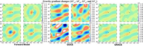
Based on the forward-modeled TSH coefficients, the coseismic gravity changes Δg and gravity gradient changes of the components (ΔVxx, ΔVyy, ΔVzz, and ΔVxz) in the LNOF on a sphere with a height of 260 km above the WGS84 reference ellipsoid were computed, which are shown in Figure 5 and Figure 6. Figure 5 shows that the magnitude of the forward-modeled coseismic gravity changes is approximately 1.2 μGal. The maximum magnitude of the components (ΔVxx, ΔVyy, ΔVzz, and ΔVxz) is approximately 0.1 mE, which corresponds to the radial component. Compared to Figure 3 and Figure 4, the spatial patterns of Figure 5 and Figure 6 are no longer dipole patterns, and instead show multiple extrema. Additionally, the gravity changes Δg and the changes in the gravity gradient components ΔVyy and ΔVzz show multiple rings. The spatial patterns of Δg and ΔVzz are very similar and nearly isotropic. According to Figure 6, the components (ΔVxx, ΔVyy, ΔVzz, and ΔVxz) have different spatial patterns. The components ΔVxx and ΔVxz have similar spatial patterns, namely, nearly west-to-east stripes and multiple poles in the North-South direction. The ΔVyy component has a spatial pattern with nearly North-South stripes and multiple poles in the west-to-east direction. Moreover, we also use two other fault slip models, provided by the GSI (Geospatial Information Authority of Japan) and the USGS (United States Geological Survey), to compute the coseismic gravity gradient changes from the TSH coefficients(see the supplementary materials). Compared with the Caltech fault slip model (as mentioned in Section 2.5), the GSI and USGS models have different depth extends. The slips extend to 70 km and 58 km in depth for the GSI and USGS models, respectively, while for the Caltech model, the maximum depth of slip is 47 km. The dip angles of the three slip models are very close, all around 10°. Although calculated with different fault slip models, the spatial patterns of the gravity and gravity gradient changes are similar to the signals plotted in Figure 5 and Figure 6.
3.2. Post-seismic Gravity Changes from the Viscoelastic Model
We compute the 1-year mean post-seismic radial gravity gradient changes (ΔVzz) based on the TSH coefficients method from the computed viscoelastic relaxation models in Section 2.6, which are shown in Figure 7. A Gaussian filter with the smoothing radius 210 km is applied to the TSH coefficients. The maximum and minimum values of the radial gravity gradient changes from the viscoelastic relaxation model are 0.0095 mE, and -0.0047 mE, respectively. This 1-year mean field will be used in removing the post-seismic effect, and deriving the coseismic gravity signals both from the GOCE and GRACE data (in Section 3.4 and Section 3.5). Comparison between our viscoelastic relaxation results and those from Han et al. [46] under the SH degree 60 truncation has also been provided in the supplementary of the manuscript.
3.3. Coseismic Gravity Changes from the Hydrological and Oceanic Mass Redistributions
Based on the TSH coefficients method, we compute the coseismic radial gravity gradient changes (ΔVzz), which are shown in Figure 8. According to Figure 8, the radial gravity gradient changes derived from the hydrological and oceanic mass redistributions are very small. The maximum and minimum value of the radial gravity gradient changes from both of GLDAS and ECCO-OBP are 0.0022 mE, and −0.0027 mE, respectively. Nevertheless, the contribution from the hydrological and oceanic mass redistributions will be removed in deriving the coseismic gravity signals both from GOCE and GRACE data.
3.4. GRACE-derived Coseismic Gravity Changes and Gravity Gradient Changes
The coseismic gravity changes and gravity gradient changes from GRACE are shown in Figure 9 and Figure 10. It should be noted that before computing the coseismic gravity changes, we removed the post-seismic effects from the one-year mean post-seismic model, and the contribution from the hydrological and oceanic mass redistributions. According to Figure 9 and Figure 10, the coseismic gravity and gravity gradient changes from GRACE have nearly the same spatial pattern, showing only clear multi-pole characteristics in the North-South direction alongside west-to-east stripes. Only the gravity gradient changes ΔVxx and ΔVxz have similar spatial patterns compared to the forward-modeled coseismic signals plotted in Figure 6. Additionally, the gravity changes and the gravity gradient components ΔVyy and ΔVzz have very different spatial patterns compared to those from the forward-modeled coseismic signals. The spatial stripes for the component ΔVyy are oriented west-to-east, which is completely different from the North-South stripes of the forward-modeled coseismic signal. The reason for this situation should be that GRACE’s satellite is in a polar orbit with an inclination of 89.5°, so the inter-satellite range-rate observations along the orbit are almost in the North-South direction. Thus, these inter-satellite range-rate observations are not sensitive to signals in the west-to-east direction.
3.5. GOCE-derived Coseismic Gravity Changes and Gravity Gradient Changes
We use the same method of processing the forward-modeled coseismic signals to compute the coseismic gravity and gravity gradient changes from GOCE, which are shown in Figure 11 and Figure 12. The post-seismic effects and the contribution from the hydrological and oceanic mass redistributions are also removed like GRACE-derived coseismic gravity signals. A Gaussian filter with a radius of 210 km was also applied. Figure 11 shows that the magnitude of the forward-modeled coseismic gravity changes is approximately 2.4 μGal. The maximum magnitude of the components (ΔVxx, ΔVyy, ΔVzz, and ΔVxz) is approximately 0.15 mE, which corresponds to the radial component.
4. Discussion
When compared to the forward-modeled coseismic signals in Figure 7 and Figure 8, the spatial patterns of the coseismic signals in Figure 11 and Figure 12 from the GOCE observations, although noisy, are somewhat similar, exhibiting multiple extrema. The spatial patterns of the gravity changes Δg and gravity gradient changes of the radial component ΔVzz exhibit multiple rings. According to Figure 12, the components ΔVxx and ΔVxz show similar spatial patterns, i.e., the west-to-east stripes and multiple poles in the North-South direction. Note that, there are more gravity gradient change peaks compared to the modeled gravity gradient changes in the area of interest, which is the same situation with Figure 8 in Fuchs et al. [28]. Referring to Fuchs et al. [28], we also use the averaged accuracy of gravity gradients before the 2011 earthquake to represent the accuracy of the derived coseismic gravity gradients. The deviations of the mean (1σ) in 0.5° grid cells for the differences of gravity gradients (ΔVxx, ΔVyy, ΔVzz and ΔVxz) between the GOCE-derived pre-earthquake model and the GOCO03S [32] are computed, which are 0.018, 0.022, 0.036 and 0.024 mE, respectively. According to Figure 12, we could see that there is a significant change (greater than 3σ) in gravity gradients between pre- and post-earthquake gravity gradients.
We note that the uncertainties (σ) might be underestimated because the two models are not completely independent and the errors are not stationary, but we will not do further assessment here. Additionally, according to Figure 5, Figure 6, Figure 11 and Figure 12, the amplitudes of the coseismic gravity gradient changes are larger than the forward-modeled coseismic signals, and the geographical positions of the multi-poles are different, which is similar to what is seen in Fuchs et al. [28]. The geographic positions of these multi-poles from the GOCE data are located approximately 200 km to the northeast of the modeled results. The reasons for these discrepancies are still not very clear. According to Fuchs et al. [28], Heki et al. [51] and Feng et al. [52], the differences between the results from the forward model and GOCE data might be caused by systematic errors in the SGG observations and the weak sensitivity of SGG observations to the location of the earthquake. In addition, the large uncertainties of fault slip models also contribute to the discrepancies. Dai et al. [16] show that the fault slip model still leads to around 40% relative difference of gravity changes compared to the GRACE observations, even inverted with a multiple data source, which is likely, because the current commonly-used dislocation models are not sophisticated enough. The noticeable differences between model prediction and observation need to be investigated by further studies. According to Figure 7, Figure 10 and Figure 12, the maximum and minimum values from the viscoelastic relaxation model are nearly 15–21% of the ones (max: 0.031 mE, min: −0.046 mE) derived from the GRACE one-year mean field differences, and nearly 3–6% of the ones (max: 0.161 mE, min: −0.167 mE) derived from the GOCE one-year mean field differences. According to Figure 8 and Figure 12, the maximum and minimum value of the radial gravity gradient changes from both of GLDAS and ECCO-OBP are nearly two orders of magnitude smaller than the GOCE-derived coseismic gravity gradient signals.
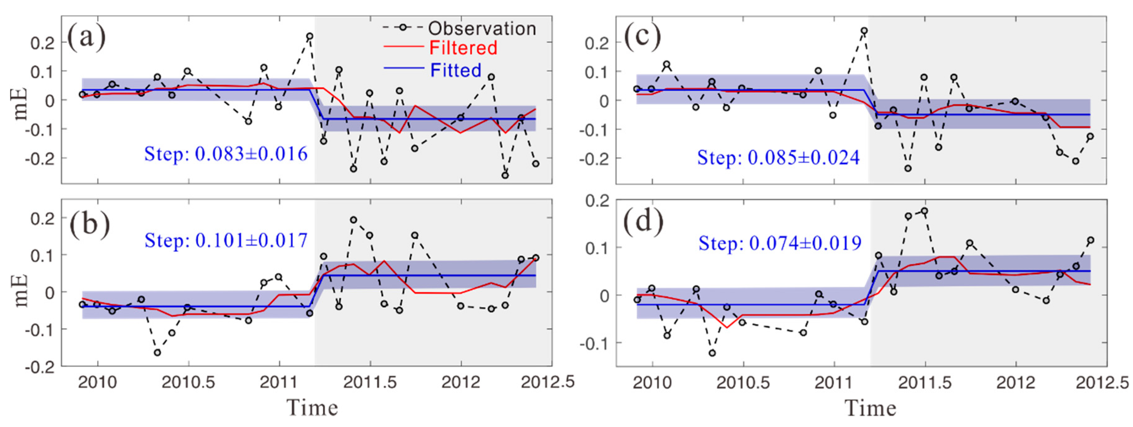
In order to show the gravity change time series, we processed the GOCE SGG data to obtain the monthly gravity field models with the time period from November 2009 to May 2012. The data processing strategies are the same with that determining the pre-earthquake and post-earthquake models above. According to the GOCE daily reports EGG [53], there are a lot of special events, several data gaps and frequent calibrating operations (about once a month), from November 2009 to May 2012. Therefore, we are unlikely to be able to derive continuous monthly time-variable gravity field models due to the practical data quality. In addition, the solutions after the earthquake have larger oscillations, which agree with the fact that there are more special events in SGG data after the earthquake than those before the earthquake for most months [53]. Figure 13a,b show the radial gravity gradient changes at A (40.6°, 141.2°) and B (40.2°, 147.2°) points on Figure 12 derived from the monthly time-variable gravity field models before and after the earthquake, while Figure 13c,d shows the average radial gravity gradient changes at a negative area [(40°~41°), (140.5°~142.5°)] around A and a positive area [(39°~40.5°), (147~148.5°)] around B.
According to Figure 13, although the radial gravity gradient change time series contain some significant oscillations, they are still comparable with the co-seismic gravity change time series from GRACE for some smaller earthquake (Mw ≈ 8.5) given by some previous studies (see as Figure 2 of Han et al. [54], and Figure 6 and Figure 7 of Chao and Liau [55]). In order to show the changes more clearly, we use a 1D median filter (with 5th order) to process those four time series, and the obtained filtered results denoted by the red curves in Figure 13. Those filtered curves show obvious steps before and after (gray areas in Figure 13) the earthquake. We further use step functions to fit the original observations (the obtained fitting curves are also plotted in Figure 13; blue curves), and the step values can be estimated at the same time (see Figure 13). Here we use a bootstrap procedure (a Monte Carlo process, see Efron and Tibshirani [56]) to estimate the uncertainties for those step values. This method has been widely used for the uncertainty estimations in different geophysical research [57,58,59,60,61,62]. Here we give a simple example to explain the error estimation process (more details can be found in Shen and Ding [60]):
- (1)
- A step function s(t) is used to fit the original time series (the earthquake time is used as a priori information in the way some previous studies have done), then the step value s is obtained at the same time.
- (2)
- 300 different random Gaussian white noise time series ni(t) are synthesized, which have the same length, and with the same mean power in the frequency domain (i.e., almost the same noise level; here we use mean power P = 1.3 × 10⁻² mE2/cpy; see the supplementary Figure S3). Note that here we ignore the small differences of the oscillation amplitudes in the radial gravity gradient change time series (see Figure 13), because the time points are limited, the 300 different noise time series can almost reproduce all possible different oscillations.
- (3)
- The fitted step function s(t) is added in the 300 noise time series ni(t), and 300 new noisy time series fi(t) = s(t) + ni(t) are obtained.
- (4)
- For the 300 noisy time series fi(t), repeating the process 1) and 2) for all of them, then the 300 new step values si can be estimated. The standard deviation of those different Si is used as the final error estimation for the step value s.
From Figure 13, we can see that the step values are clearly over three times their corresponding uncertainties (the double uncertainties are denoted by the blue areas in Figure 13 as the corresponding two standard deviations). Statistically, we may suggest that those steps represent the coseismic gravity gradient change signals caused by the 2011 Tohoku-Oki earthquake.
To reveal how the spatial patterns of the GOCE and modeled gravity gradient changes agree with each other, we computed the correlation coefficients (see Table 2) of the gravity changes and gravity gradient changes (ΔVxx, ΔVyy, ΔVzz, ΔVxz and Δg) between the observed models (GOCE and GRACE) and the forward model for the TSH coefficients (see Figure 2). The Root Mean Square (RMS) of observed (ΔVxx, ΔVyy, ΔVzz, ΔVxz and Δg) of GOCE/GRACE, and the differences between the observed and forward modeling signals, are also computed and shown in Table 2. According to Table 2, both of GOCE and GRACE do not perform well, because all the correlation coefficients are less than or equal to 0.85. Although most correlation coefficients corresponding to GOCE are lower than those of the GRACE time-variable gravity field models, the correlation coefficient corresponding to the ΔVyy component from GOCE is slightly larger than the one of GRACE. Thus, for the SH degree range 30–95, the GOCE mission could reveal a greater signal of coseismic gravity gradient changes in the west-to-east direction than GRACE, because GRACE has sensitive observations along the North-South direction. The coefficient for ΔVzz is very close to the value in Fuchs et al. [28]. All RMS of observed signals are reduced after subtracting the forward-modeled coseismic signals from the GOCE-derived results. However, because the amplitude of the results from GRACE is only about half of the one from the forward model, the RMS of GRACE’s ΔVyy increases when the modeled signal is subtracted from the observed signal and the RMS of ΔVyy doesn’t change. Of course, compared to GOCE, GRACE performs relatively well in the SH degree range 30–95, especially for the ΔVxx component, which has the maximum correlation coefficient because only inter-satellite range-rates are observed along its orbit.
5. Conclusions
We employed the least squares method with a bandpass auto regression moving average filter, to recover two global gravity field models up to degree and order 220, from GOCE satellite gravity gradient data from the 15 March 2011 to the 31 May 2012 after the 2011 Japan Tohoku-Oki earthquake event. Then, we used the recovered models to estimate the coseismic gravity and gravity gradient changes that were caused by the earthquake by subtracting the pre-earthquake model from the post-earthquake model. This approach is different from that in Fuchs et al. [28]. They used the diagonal components (Vxx, Vyy, and Vzz) along the orbit to construct the new vertical gravity gradient Vzz, which was used to present the coseismic gravity gradient changes. To extract the coseismic gravity signals from the recovered global gravity field models, we proposed TSH coefficients according to the influences of colored noise in the SGG data and the polar gap problem on the recovered models.
The gravity changes Δg and the gravity gradient changes (ΔVxx, ΔVyy, ΔVzz, and ΔVxz) were computed by the GOCE-derived tailored spherical harmonic (TSH) coefficients, GRACE-derived TSH coefficients and the forward-modeled TSH coefficients. In data processing, the degree range 30–95 was used to obtain the TSH coefficients. A Gaussian filter with a radius of 210 km was also applied to the TSH coefficients according to the maximum frequency of 95. When comparing the coseismic gravity signals from GOCE, the forward model, and GRACE, the spatial patterns of the coseismic gravity and gravity gradient changes from GOCE were analogous to those from the forward model. There is a significant change (greater than 3σ) in the gravity gradients between the pre- and post-earthquake gravity gradients, which is associated with the earthquake. Moreover, the radial gravity gradient changes from the derived monthly time-variable gravity field models before and after the earthquake show obvious steps before and after the earthquake, whose amplitudes are at a level over three times that of their corresponding uncertainties, and thus significant. Statistically, it is reasonable to infer that these steps represent the coseismic gravity gradient change signals caused by the 2011 Tohoku-Oki earthquake. For the GGT components (ΔVxx, ΔVzz, and ΔVxz), the correlation between the GOCE-derived coseismic gravity signals and the forward-modeled coseismic results was weaker than that from GRACE. However, the correlation coefficient that corresponded to the ΔVyy component from GOCE is larger than that from GRACE. The component ΔVyy had spatial patterns that included North-South stripes and multiple poles in the west-to-east direction. This situation means that the GOCE mission might reveal more coseismic gravity signals in the West-East direction than GRACE in the SH degree range 30–95. The estimated time series of radial gravity gradient changes (see Figure 13) suggest that the coseismic gravity changes can be reproduced from GOCE observations through the proposed method.
Supplementary Materials
The following are available online at https://www.mdpi.com/2072-4292/11/11/1295/s1, Figure S1: Gravity gradient changes (ΔVxx, ΔVyy, ΔVzz, and ΔVxz) in LNOF on a sphere with a height of 260 km computed by the TSH coefficients from the forward-modeled signals of the GSI fault slip model with a Gaussian filter applied, Figure S2: Gravity gradient changes (ΔVxx, ΔVyy, ΔVzz, and ΔVxz) in LNOF on a sphere with a height of 260 km computed by the TSH coefficients from the forward-modeled signals of the USGS fault slip model with a Gaussian filter applied, Figure S3: The observation (the fitted step has been removed) and the inputted noise (a), and their Fourier power spectra (b) (logarithmic scale in dB), Figure S4: Postseismic gravity changes (Δg) on the ground from the spherical harmonic coefficients up to d/o 60 of the viscoelastic relaxation model computed in the paper (left) and provided by Han (right).
Author Contributions
Conceptualization X.X.; methodology, X.X. and H.D.; investigation, X.X. and H.D.; resources, J.L. and M.H.; data curation, Y.Z.; writing—original draft preparation, X.X.; writing—review and editing, X.X., H.D., and J.L.
Funding
This research was financially supported by the National Natural Science Foundation of China (Grant No. 41574019, 41774020, 11873075). DAAD Thematic Network Project (57421148). The Major Project of High resolution Earth Observation System. The Natural Science Foundation of Shanghai (17ZR1435600).
Acknowledgments
The authors thank Shin-Chan Han for the help in our post-seismic effect evaluation and providing the viscoelastic and afterslip models of the Tohuku-Oki earthquake for the verification of our post-seismic models. We thank Wenbin Shen for useful discussion. We also acknowledge the European Space Agency for providing the GOCE data. We are also grateful to the three anomalous reviewers who have provided constructive comments and suggestions to improve our work.
Conflicts of Interest
The authors declare no conflict of interest.
References
- Reigber, C.; Schwintzer, P.; Neumayer, K.H.; Barthelmes, F.; König, R.; Förste, C.; Balmino, G.; Biancale, R.; Lemoine, J.-M.; Loyer, S.; et al. The CHAMP-only earth gravity field model EIGEN-2. Adv. Space Res. 2003, 31, 1883–1888. [Google Scholar] [CrossRef]
- Tapley, B.D.; Bettadpur, S.; Watkins, M.; Reigber, C. The gravity recovery and climate experiment: Mission overview and early results. Geophys. Res. Lett. 2004, 31, L09607. [Google Scholar] [CrossRef]
- Drinkwater, M.; Haagmans, R.; Muzi, D. The GOCE gravity mission: ESA’s first core explorer. In Proceedings of the Third GOCE User Workshop, Frascati, Italy, 6–9 November 2006; pp. 1–7. [Google Scholar]
- Han, S.C.; Shum, C.K.; Bevis, M.; Ji, C.; Kuo, C.Y. Crustal dilatation observed by GRACE after the 2004 Sumatra-Andaman earthquake. Science 2006, 313, 658–662. [Google Scholar] [CrossRef]
- Chen, J.L.; Wilson, C.R.; Tapley, B.D.; Grand, S. GRACE detects coseismic and postseismic deformation from the Sumatra-Andaman earthquake. Geophys. Res. Lett. 2007, 34, L13302. [Google Scholar] [CrossRef]
- Panet, I.; Pollitz, F.; Mikhailov, V.; Diament, M.; Banerjee, P.; Grijalva, K. Upper mantle rheology from GRACE and GPS postseismic deformation after the 2004 Sumatra-Andaman earthquake. Geochem. Geophys. Geosyst. 2010, 11, Q06008. [Google Scholar] [CrossRef]
- De Linage, C.; Rivera, L.; Hinderer, J.; Boy, J.P.; Rogister, Y.; Lambotte, S.; Biancale, R. Separation of coseismic and postseismic gravity changes for the 2004 Sumatra-Andaman earthquake from 4.6 yr of GRACE observations and modeling of the coseismic change by normal modes summation. Geophys. J. Int. 2009, 176, 695–714. [Google Scholar] [CrossRef]
- Han, S.C.; Sauber, J.; Luthcke, S. Regional gravity decrease after the 2010 Maule (Chile) earthquake indicates large-scale mass redistribution. Geophys. Res. Lett. 2010, 37, L23307. [Google Scholar] [CrossRef]
- Heki, K.; Matsuo, K. Coseismic gravity changes of the 2010 earthquake in central Chile from satellite gravimetry. Geophys. Res. Lett. 2010, 37, L24306. [Google Scholar] [CrossRef]
- Broerse, D.; Vermeersen, L.; Riva, R.; van der Wal, W. Ocean contribution to co-seismic crustal deformation and geoid anomalies: Application to the 2004 December 26 Sumatra-Andaman earthquake. Earth Planet. Sci. Lett. 2011, 305, 341–349. [Google Scholar] [CrossRef]
- Matsuo, K.; Heki, K. Coseismic gravity changes of the 2011 Tohoku-Oki earthquake from satellite gravimetry. Geophys. Res. Lett. 2011, 38, L00G12. [Google Scholar] [CrossRef]
- Han, S.C.; Sauber, J.; Riva., R. Contribution of satellite gravimetry to understanding seismic source processes of the 2011 Tohoku-Oki earthquake. Geophys. Res. Lett. 2011, 38, L24312. [Google Scholar] [CrossRef]
- Wang, L.; Shum, C.K.; Simons, F.J.; Tapley, B.; Dai, C. Coseismic and postseismic deformation of the 2011 Tohoku-Oki earthquake constrained by GRACE gravimetry. Geophys. Res. Lett. 2012, 39, L07301. [Google Scholar] [CrossRef]
- Zhou, X.; Sun, W.; Zhao, B.; Fu, G.; Dong, J.; Nie, Z. Geodetic observations detecting coseismic displacements and gravity changes caused by the Mw = 9.0 Tohoku-Oki earthquake. J. Geophys. Res. 2012, 117, B05408. [Google Scholar] [CrossRef]
- Cambiotti, G.; Sabadini, R. A source model for the great 2011 Tohoku earthquake (Mw = 9.1) from inversion of GRACE gravity data. Earth Planet Sci. Lett. 2012, 335–336, 72–79. [Google Scholar] [CrossRef]
- Dai, C.; Shum, C.K.; Wang, R.; Wang, L.; Guo, J.; Shang, K.; Tapley, B.D. Improved constraints on seismic source parameters of the 2011 Tohoku earthquake from GRACE gravity and gravity gradient changes. Geophys. Res. Lett. 2014, 41, 1929–1936. [Google Scholar] [CrossRef] [Green Version]
- Li, J.; Shen, W.B. Monthly GRACE detection of coseismic gravity change associated with 2011 Tohoku-Oki earthquake using northern gradient approach. Earth Planets Space 2015, 67, 29. [Google Scholar] [CrossRef]
- Odera, P.A.; Fukuda, Y. Evaluation of GOCE-based global gravity field models over Japan after the full mission using free-air gravity anomalies and geoid undulations. Earth Planets Space 2017, 69, 135. [Google Scholar] [CrossRef] [Green Version]
- Gilardoni, M.; Reguzzoni, M.; Sampietro, D.; Sansò, F. Combining EGM2008 with GOCE gravity models. Bollettino di Geofisica Teorica ed Applicata 2013, 54, 285–302. [Google Scholar]
- Bouman, J.; Ebbing, J.; Martin Fuchs, M.J.; Sebera, J.; Lieb, V.; Szwillus, W.; Haagmans, R.; Novak, P. Satellite gravity gradient grids for geophysics. Sci. Rep. 2016, 6, 21050. [Google Scholar] [CrossRef] [Green Version]
- Bouman, J.; Ebbing, J.; Meekes, S.; Fattah, R.A.; Fuchs, M.; Gradmann, S.; Haagmans, R.; Lieb, V.; Schmidt, M.; Dettmering, D.; et al. GOCE gravity gradient data for lithospheric modeling. Int. J. Appl. Earth Obs. 2015, 35, 16–30. [Google Scholar] [CrossRef]
- Reguzzoni, M.; Sampietro, D. GEMMA: An Earth crustal model based on GOCE satellite data. Int. J. Appl. Earth Obs. 2015, 35, 31–43. [Google Scholar] [CrossRef]
- Bingham, R.J.; Haines, K.; Lea, D. A comparison of GOCE and drifter-based estimates of the North Atlantic steady-state surface circulation. Int. J. Appl. Earth Obs. 2015, 35, 140–150. [Google Scholar] [CrossRef]
- Mikhailov, V.; Tikhotsky, S.; Diament, M.; Panet, I.; Ballu, V. Can tectonic processes be recovered from new gravity satellite data? Earth Planet Sci. Lett. 2004, 228, 281–297. [Google Scholar] [CrossRef]
- Migliaccio, F.; Reguzzoni, M.; Sansò, F.; Dalla Via, G.; Sabadini, R. Detecting geophysical signals in gravity satellite missions. Geophys. J. Int. 2008, 172, 56–66. [Google Scholar] [CrossRef] [Green Version]
- Han, S.-C.; Ditmar, P. Localized spectral analysis of global satellite gravity fields for recovering time-variable mass redistributions. J. Geod. 2008, 82, 423–430. [Google Scholar] [CrossRef]
- Garcia, R.F.; Bruinsma, S.; Lognonné, P.; Doornbos, E.; Cachoux, F. GOCE: The First Seismometer in Orbit around the Earth. Geophys. Res. Lett. 2013. [Google Scholar] [CrossRef]
- Fuchs, M.J.; Bouman, J.; Broerse, T.; Visser, P.; Vermeersen, B. Observing coseismic gravity change from the Japan Tohoku-Oki 2011 earthquake with GOCE gravity gradiometry. J. Geophys. Res. Solid Earth. 2013, 118, 5712–5721. [Google Scholar] [CrossRef] [Green Version]
- Fuchs, M.J.; Hooper, A.; Broerse, T.; Bouman, J. Distributed fault slip model for the 2011 Tohoku-Oki earthquake from GNSS and GRACE/GOCE satellite gravimetry. J. Geophys. Res. Solid Earth. 2016, 121, 1114–1130. [Google Scholar] [CrossRef]
- Han, S.C.; Shum, C.K.; Ditmar, P.; Visser, P.; van Beelen, C.; Schrama, E.J.O. Effect of high-frequency mass variations on GOCE recovery of the Earth’s gravity field. J. Geodyn. 2006, 41, 69–76. [Google Scholar] [CrossRef]
- Bouman, J.; Fiorot, S.; Fuchs, M.; Gruber, T.; Schrama, E.; Tscherning, C.C.; Veicherts, M.; Visser, P. GOCE gravity gradients along the orbit. J. Geod. 2011, 85, 791–805. [Google Scholar] [CrossRef]
- Mayer-Gürr, T.; Rieser, D.; Hoeck, E.; Brockmann, J.M.; Schuh, W.-D.; Krasbutter, I.; Kusche, J.; Maier, A.; Krauss, S.; Hausleitner, W.; et al. The new combined satellite only model GOCO03s. Presented at the GGHS2012, Venice, Italy, 9–12 November 2012. [Google Scholar]
- Xu, X.; Zhao, Y.; Reubelt, T.; Tenzer, R. A GOCE only gravity model GOSG01S and the validation of GOCE related satellite gravity models. Geod. Geodyn. 2017, 8, 260–272. [Google Scholar] [CrossRef]
- Koop, R. Global Gravity Field Modeling Using Satellite Gravity Gradiometry; Publications on Geodesy, New Series, Number 38; Netherlands Geodetic Commission: Delft, The Netherlands, 1993. [Google Scholar]
- Cesare, S. Performance Requirements and Budgets for the Gradiometric Mission; Technical Note, GOC-TN-AI-0027; Alenia Spazio: Turin, Italy, 2008. [Google Scholar]
- Schuh, W.D. Improved modelling of SGG-data sets by advanced filter strategies. In ESA-Project “From Eötvös to mGal+”; Final Report, ESA/ESTEC Contract 14287/00/NL/DC, WP 2; ESA: Noordwijk, The Netherlands, 2002; pp. 113–181. [Google Scholar]
- Fuchs, M.; Bouman, J. Rotation of GOCE gravity gradients to local frames. Geophys. J. Int. 2011, 187, 743–753. [Google Scholar] [CrossRef] [Green Version]
- Rummel, R.; Yi, W.; Stummer, C. GOCE gravitational gradiometry. J. Geod. 2011, 85, 777–790. [Google Scholar] [CrossRef]
- Sneeuw, N.; van Gelderen, M. The polar gap. In Geodetic Boundary Value Problems in View of the One Centimeter Geoid; Sansò, F., Rummel, R., Eds.; Lecture Notes in Earth Sciences; Springer: Berlin, Germany, 1997; Volume 65, pp. 559–568. [Google Scholar]
- EGG-C. GOCE Level 2 Product Data Handbook; GO-MA-HPF-GS-0110. 2010. Available online: https://earth.esa.int/web/guest/document-library/browse-document-library/-/article/goce-level-2-product-data-handbook-5713 (accessed on 12 May 2017).
- Wang, R.; Lorenzo-Martiín, F.; Roth, F. PSGRN/PSCMP—A new code for calculating co- and post-seismic deformation, geoid and gravity changes based on the viscoelastic-gravitational dislocation theory. Comput. Geosci. 2006, 32, 527–541. [Google Scholar] [CrossRef]
- Wei, S.; Sladen, A.; The ARIA Group. Updated Result: 3/11/2011 (Mw 9.0), Tohoku-Oki, Japan. 2011. Available online: http://www.tectonics.caltech.edu/slip_history/2011_taiheiyo-oki/ (accessed on 18 June 2015).
- Bassin, C.; Laske, G.; Masters, G.G. The current limits of resolution for surface wave tomography in North America. EOS Trans. 2000, 81, F897. [Google Scholar]
- Broerse, T.; Riva, R.; Vermeersen, B. Ocean contribution to seismic gravity changes: The sea level equation for seismic perturbations revisited. Geophys. J. Int. 2014, 199, 1094–1109. [Google Scholar] [CrossRef]
- Colombo, O. Numerical Methods for Harmonic Analysis on the Sphere; Report No. 310; Dept. of Geodetic Science and Surveying, Ohio State University: Columbus, OH, USA, 1981. [Google Scholar]
- Han, S.-C.; Sauber, J.; Pollitz, F. Broadscale postseismic gravity change following the 2011 Tohoku-Oki earthquake and implication for deformation by viscoelastic relaxation and afterslip. Geophys. Res. Lett. 2014, 41, 5797–5805. [Google Scholar] [CrossRef]
- Bouman, J.; Rispens, S.; Gruber, T.; Koop, R.; Schrama, E.; Visser, P.; Tscherning, C.C.; Veicherts, M. Preprocessing of gravity gradients at the GOCE high-level processing facility. J. Geod. 2009, 83, 659–678. [Google Scholar] [CrossRef]
- Fukumori, I. A partitioned Kalman filter and smoother. Mon. Weather Rev. 2002, 130, 1370–1383. [Google Scholar] [CrossRef]
- Kim, S.B.; Lee, T.; Fukumori, I. Mechanisms Controlling the Interannual Variation of Mixed Layer Temperature Averaged over the Niño-3 Region. J. Clim. 2007, 20, 3822–3843. [Google Scholar] [CrossRef]
- Rodell, M.; Houser, P.R.; Jambor, U.; Gottschalck, J.; Mitchell, K.; Meng, C.-J.; Arsenault, K.; Cosgrove, B.; Radakovich, J.; Bosilovich, M.; et al. The Global Land Data Assimilation System. Bull. Am. Meteorol. Soc. 2004, 85, 381–394. [Google Scholar] [CrossRef] [Green Version]
- Heki, K.; Mitsui, Y.; Matsuo, K.; Tanaka, Y. Accelerated subduction of the Pacific Plate after mega-thrust earthquakes: Evidence from GPS and GRACE. Presented at the AGU Fall Meeting 2012, San Francisco, CA, USA, 3–7 December 2012. [Google Scholar]
- Feng, W.; Li, Q.; Li, Z.; Hoey, T. Slip distribution of 2011 Japan Mw 9.0 earthquake determined by GPS-coseismic displacement and GRACE gravity changes. Presented at the EGU Scientific Assembly, Vienna, Austria, 7–12 April 2013. [Google Scholar]
- ESA. Available online: https://earth.esa.int/web/sppa/mission-performance/esa-missions/goce/quality -control-reports/daily-egg-quality-overview (accessed on 20 January 2019).
- Han, S.-C.; Sauber, J.; Pollitz, F. Coseismic compression/dilatation and viscoelastic uplift/subsidence following the 2012 Indian Ocean earthquakes quantified from satellite gravity observations. Geophys. Res. Lett. 2015, 42, 3764–3772. [Google Scholar] [CrossRef]
- Chao, B.F.; Liau, J.R. Gravity changes due to large earthquakes detected in GRACE satellite data via empirical orthogonal function analysis. J. Geophys. Res. Solid Earth 2019. [Google Scholar] [CrossRef]
- Efron, B.; Tibshirani, R. Bootstrap methods for standard errors, confidence intervals, and other measures of statistical accuracy. Stat. Sci. 1986, 1, 54–75. [Google Scholar] [CrossRef]
- Widmer-Schnidrig, R.; Masters, G.; Gilbert, F. Observably split multiplets-data analysis and interpretation in terms of large-scale aspherical structure. Geophys. J. Int. 1992, 111, 559–576. [Google Scholar] [CrossRef] [Green Version]
- Häfner, R.; Widmer-Schnidrig, R. Signature of 3-D density structure in spectra of the spheroidal free oscillation 0S2. Geophys. J. Int. 2013, 192, 285–294. [Google Scholar] [CrossRef]
- Shen, W.B.; Ding, H. Observation of spheroidal normal mode multiplets below 1 mHz using ensemble empirical mode decomposition. Geophys. J. Int. 2014, 196, 1631–1642. [Google Scholar] [CrossRef]
- Ding, H.; Chao, B.F. Data stacking methods for isolation of singlets of the Earth’s normal modes: Extensions comparisons and applications. J. Geophys. Res. Solid Earth 2015, 120, 5034–5050. [Google Scholar] [CrossRef]
- Chen, J.L.; Wilson, C.R.; Tapley, B.D. Contribution of ice sheet and mountain glacier melt to recent sea level rise. Nat. Geosci. 2013, 6, 549–552. [Google Scholar] [CrossRef]
- Han, J.; Tangdamrongsub, N.; Hwang, C.; Abidin, H.Z. Intensified water storage loss by biomass burning in Kalimantan: Detection by GRACE. J. Geophys. Res. Solid Earth 2017, 122, 2409–2430. [Google Scholar] [CrossRef]
Figure 1.
Power spectral densities of the diagonal components (Vxx, Vyy, and Vzz) and trace of the Gravity field and steady state Ocean Circulation Explorer (GOCE) gravity gradient tensor.
Figure 1.
Power spectral densities of the diagonal components (Vxx, Vyy, and Vzz) and trace of the Gravity field and steady state Ocean Circulation Explorer (GOCE) gravity gradient tensor.

Figure 2.
Error spectra of the recovered spherical harmonic (SH) coefficients in log10 scale compared to EGM2008.
Figure 2.
Error spectra of the recovered spherical harmonic (SH) coefficients in log10 scale compared to EGM2008.
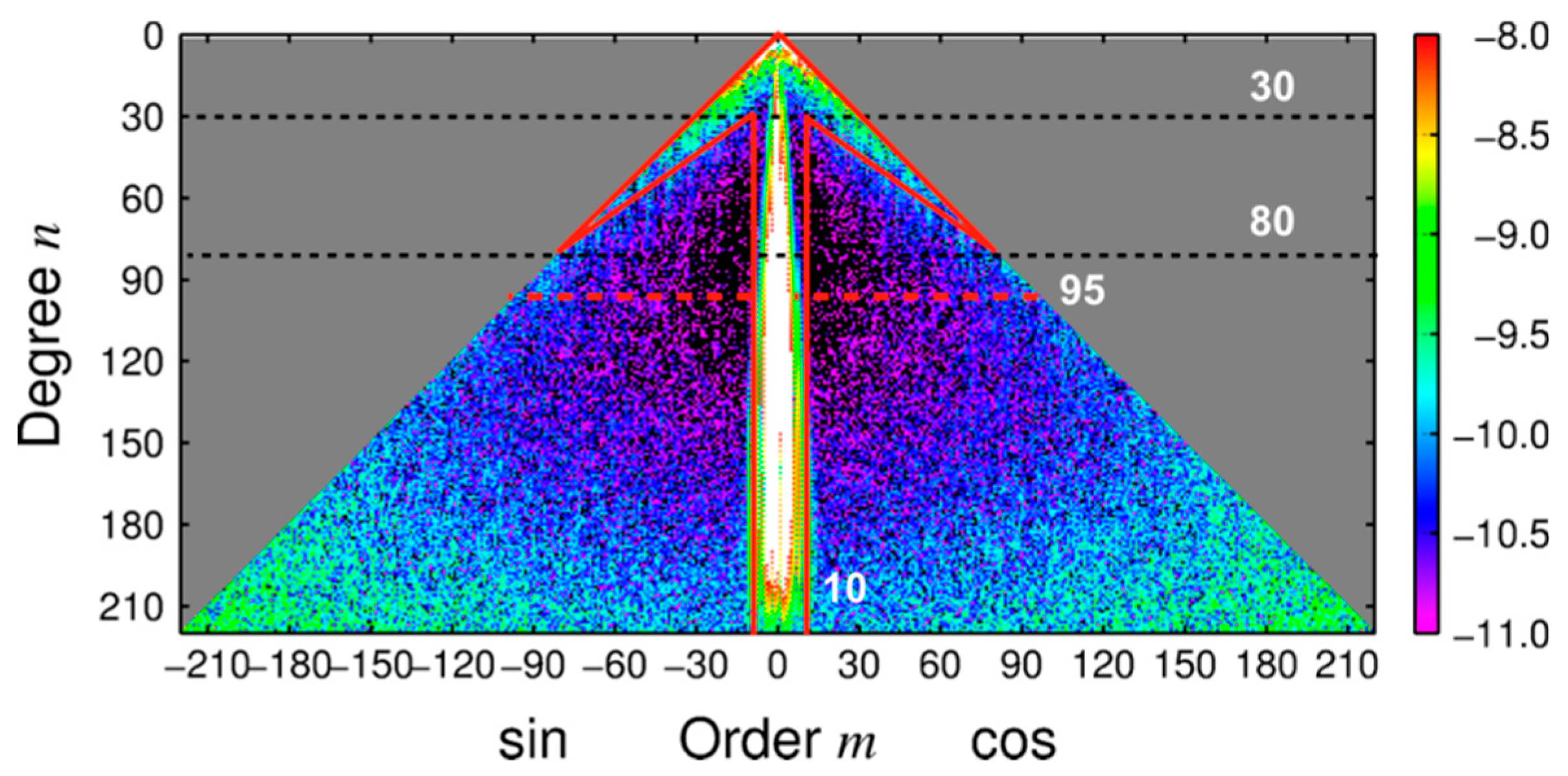
Figure 3.
Coseismic gravity changes (a) on the Earth’s surface and (b) on a sphere with a height of 260 km, when using forward-modeled spherical harmonic coefficients up to d/o 250 with a Gaussian filter applied (radius of 110 km). The units are μGal.
Figure 3.
Coseismic gravity changes (a) on the Earth’s surface and (b) on a sphere with a height of 260 km, when using forward-modeled spherical harmonic coefficients up to d/o 250 with a Gaussian filter applied (radius of 110 km). The units are μGal.

Figure 4.
Coseismic radial gravity gradient change (a) on the Earth’s surface and (b) on a sphere with a height of 260 km when using spherical harmonic coefficients up to d/o 250 with a Gaussian filter applied (radius of 110 km). The units are mE.
Figure 4.
Coseismic radial gravity gradient change (a) on the Earth’s surface and (b) on a sphere with a height of 260 km when using spherical harmonic coefficients up to d/o 250 with a Gaussian filter applied (radius of 110 km). The units are mE.

Figure 5.
Gravity changes on a sphere with a height of 260 km computed by the tailored spherical harmonic coefficients from the forward model with a Gaussian filter applied. The SH degree range is 30–95 and the radius of the filter is 210 km. The unit is μGal.
Figure 5.
Gravity changes on a sphere with a height of 260 km computed by the tailored spherical harmonic coefficients from the forward model with a Gaussian filter applied. The SH degree range is 30–95 and the radius of the filter is 210 km. The unit is μGal.
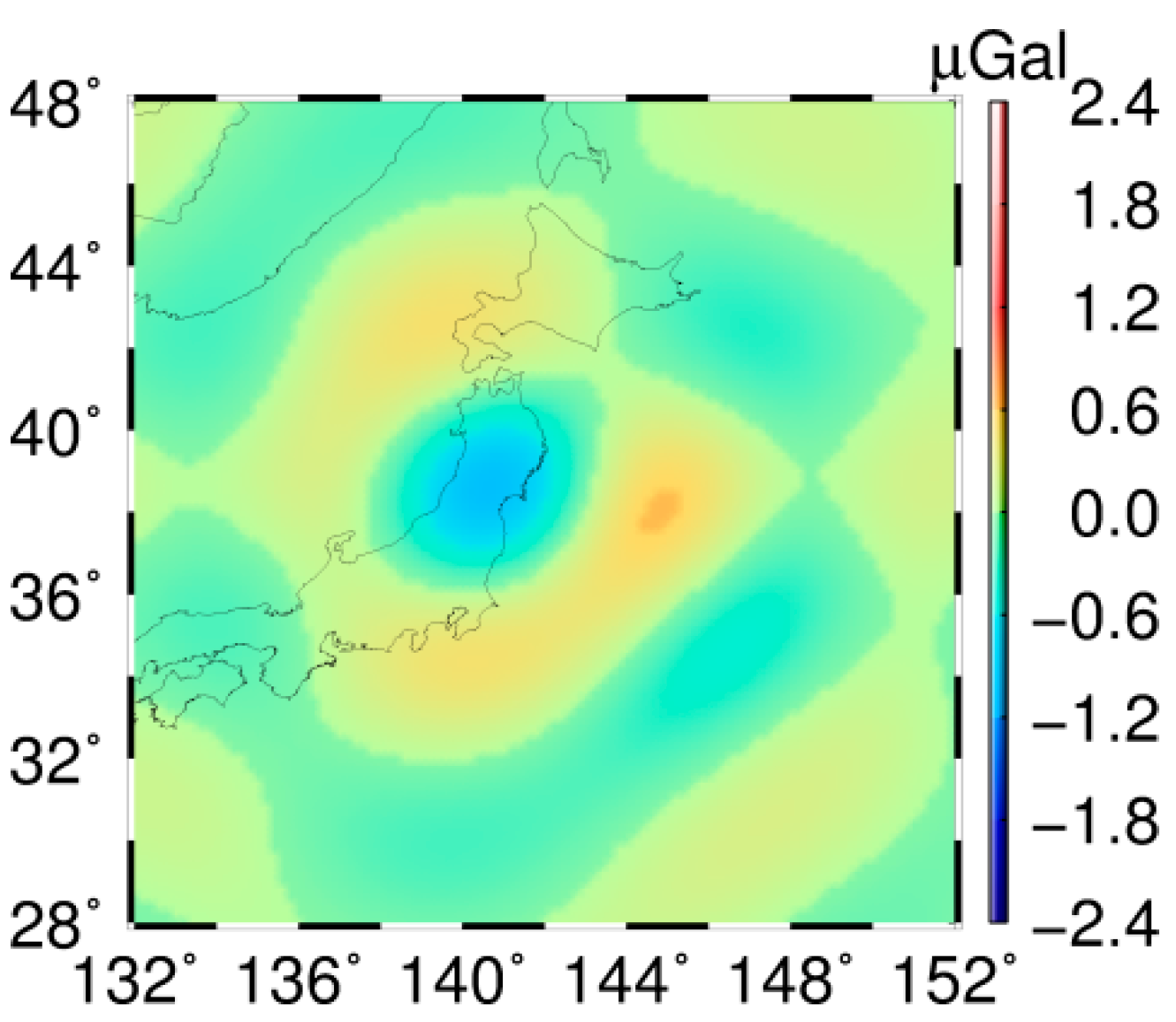
Figure 6.
Gravity gradient changes (ΔVxx, ΔVyy, ΔVzz, and ΔVxz) in Local North-Oriented Frame on a sphere with a height of 260 km computed by the tailored spherical harmonic coefficients from the forward-modeled coseismic signals with a Gaussian filter applied. The SH degree range is 30–95 and the radius of the filter is 210 km. The units are mE.

Figure 7.
Radial gravity gradient changes (ΔVzz) in Local North-Oriented Frame on a sphere with a height of 260 km computed by the tailored spherical harmonic coefficients from the viscoelastic relaxation model with a Gaussian filter applied. The SH degree range is 30–95 and the radius of the filter is 210 km. The units are mE.
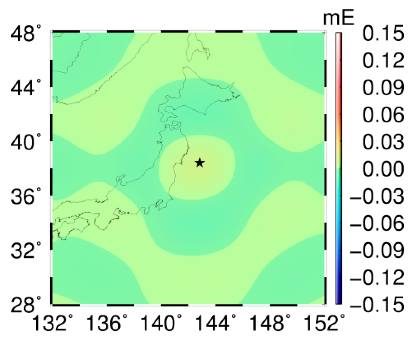
Figure 8.
Radial gravity gradient changes (ΔVzz) in Local North-Oriented Frame on a sphere with a height of 260 km computed by the tailored spherical harmonic coefficients from GLDAS (a), ECCO-OBP (b) and both of GLDAS and ECCO-OBP (c) with a Gaussian filter applied. The SH degree range is 30–95 and the radius of the filter is 210 km. The units are mE.
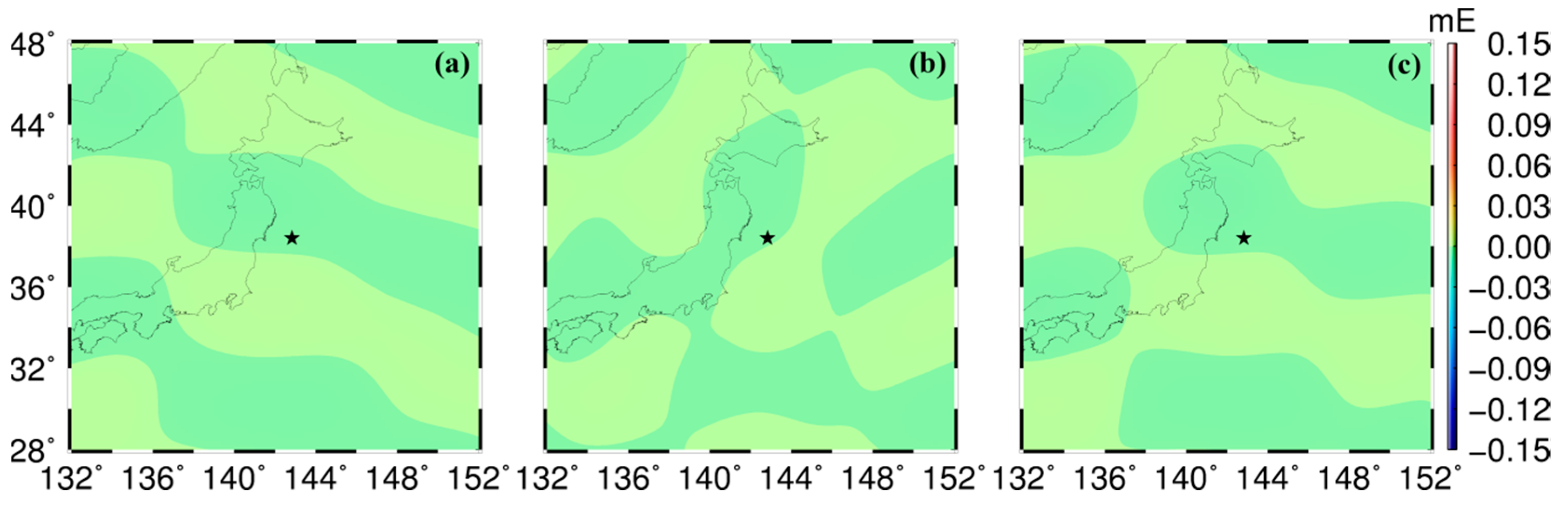
Figure 9.
Gravity changes on a sphere with a height of 260 km computed by the tailored spherical harmonic coefficients from GRACE (the Gravity field Recovery and Climate Experiment). The SH degree range is 30–95. The unit is μGal.
Figure 9.
Gravity changes on a sphere with a height of 260 km computed by the tailored spherical harmonic coefficients from GRACE (the Gravity field Recovery and Climate Experiment). The SH degree range is 30–95. The unit is μGal.
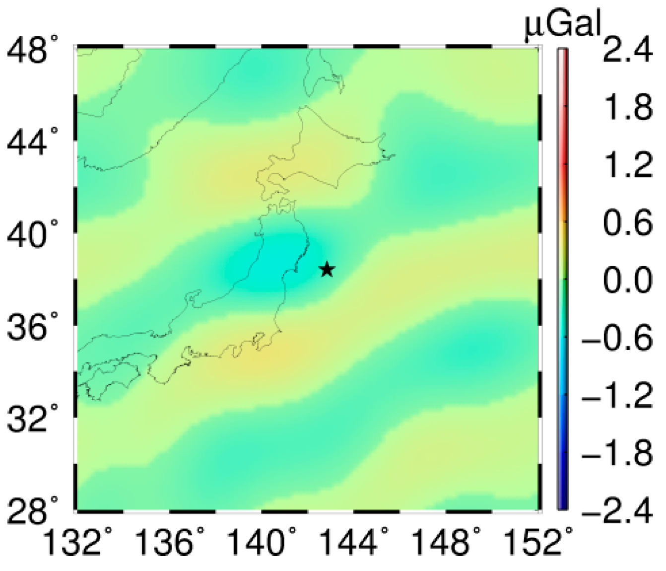
Figure 10.
Gravity gradient changes (ΔVxx, ΔVyy, ΔVzz, and ΔVxz) in Local North-Oriented Frame on a sphere with a height of 260 km computed by the tailored spherical harmonic coefficients from GRACE. The SH degree range is 30–95. The units are mE.
Figure 10.
Gravity gradient changes (ΔVxx, ΔVyy, ΔVzz, and ΔVxz) in Local North-Oriented Frame on a sphere with a height of 260 km computed by the tailored spherical harmonic coefficients from GRACE. The SH degree range is 30–95. The units are mE.
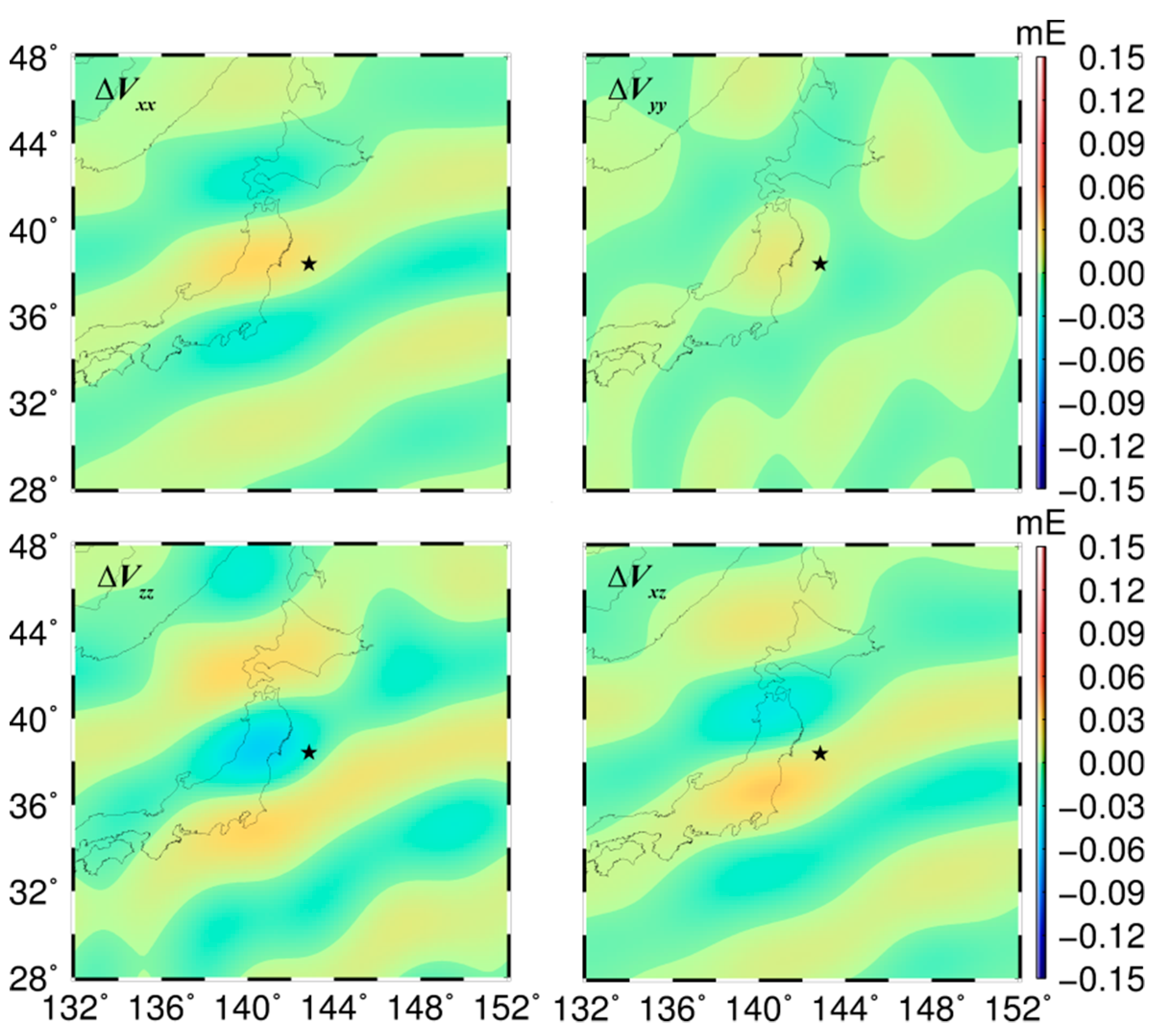
Figure 11.
Gravity changes on a sphere with a height of 260 km computed by the tailored spherical harmonic coefficients from the GOCE observations with a Gaussian filter applied. The SH degree range is 30–95, and the radius of the filter is 210 km. The unit is μGal.
Figure 11.
Gravity changes on a sphere with a height of 260 km computed by the tailored spherical harmonic coefficients from the GOCE observations with a Gaussian filter applied. The SH degree range is 30–95, and the radius of the filter is 210 km. The unit is μGal.
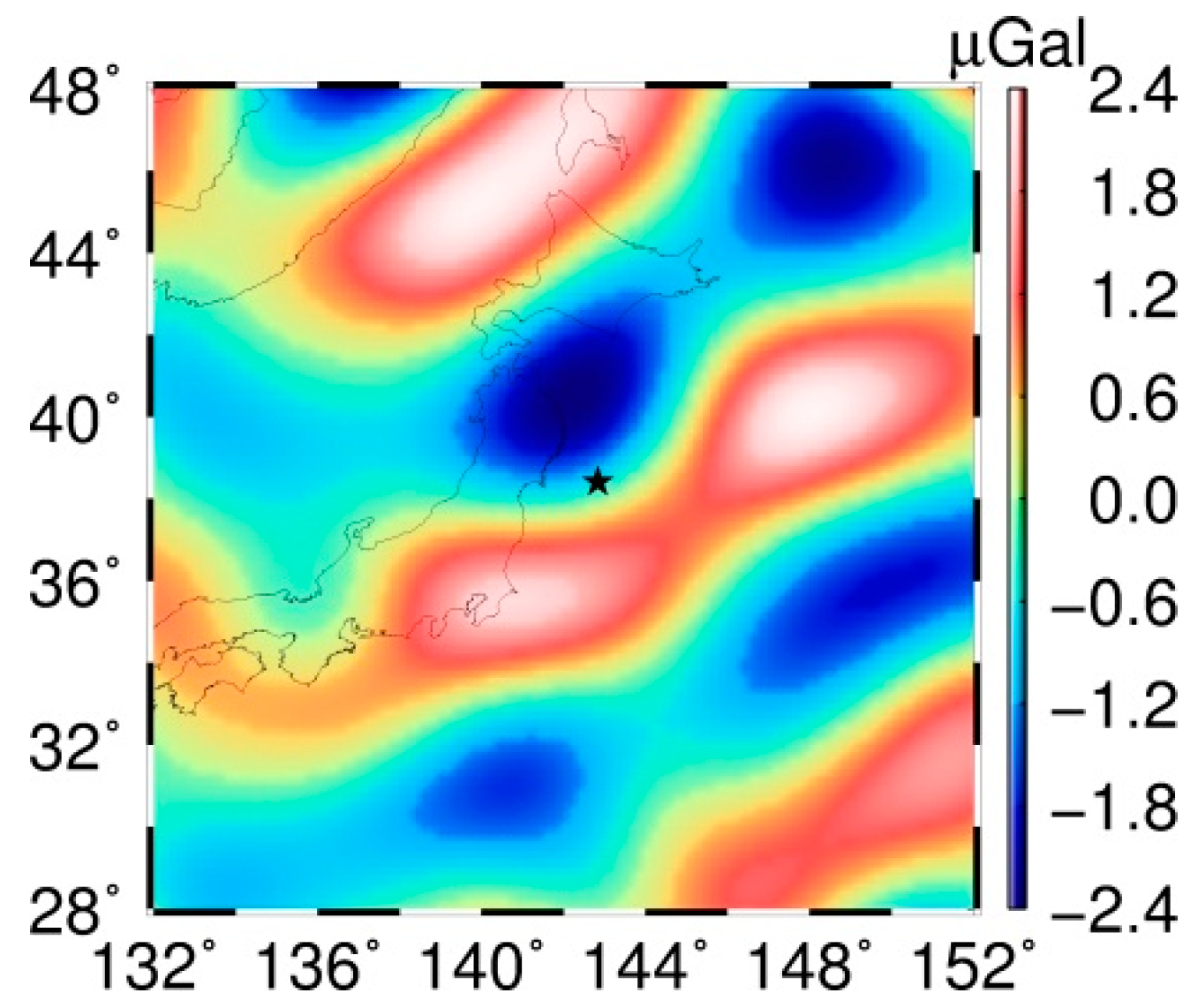
Figure 12.
Gravity gradient changes (ΔVxx, ΔVyy, ΔVzz, and ΔVxz) in Local North-Oriented Frame on a sphere with a height of 260 km computed by the tailored spherical harmonic coefficients from the GOCE observations with a Gaussian filter applied. The SH degree range is 30–95, and the radius of the filter is 210 km. The units are mE.

Figure 13.
Radial gravity gradient changes at A (a), B (b) points and two selected areas around A and B (c,d) before and after earthquake. The red curves denote the filtered results after using a 1D median filter to the original time series, the blue curves are the fitted step functions. The double uncertainties are denoted by the blue areas.

Table 1.
The 5-layer half-space Earth model used in the prediction of co- and post-seismic gravity changes.
Table 1.
The 5-layer half-space Earth model used in the prediction of co- and post-seismic gravity changes.
| Depth (km) | Density (ρ) (103 kg/m3) | VP(km/s) | VS(km/s) | Material Type |
|---|---|---|---|---|
| 0–1 | 2.10 | 2.10 | 1.00 | Elastic |
| 1–8 | 2.70 | 6.00 | 3.40 | Elastic |
| 8–15 | 2.90 | 6.60 | 3.70 | Elastic |
| 15–22 | 3.05 | 7.20 | 4.00 | Elastic |
| 22–∞ | 3.40 | 8.20 | 4.70 | Biviscous (Burgers body) |
Table 2.
Correlation coefficients, RMS of observed gravity and gravity gradients (ΔVxx, ΔVyy, ΔVzz, ΔVxz and Δg), RMS of the differences between the observed and forward modeling signals. The observed signals are from GRACE and GOCE. The positions for the computation are located in the region of 28°N–48°N, 132°E–152°E. The unit of ΔVxx, ΔVyy, ΔVzz, and ΔVxz is mE and the unit of Δg is μGal.
| GOCE | GRACE | |||||||||
|---|---|---|---|---|---|---|---|---|---|---|
| Quantities | ΔVxx | ΔVyy | ΔVzz | ΔVxz | Δg | ΔVxx | ΔVyy | ΔVzz | ΔVxz | Δg |
| Correlation coefficients | 0.68 | 0.56 | 0.61 | 0.68 | 0.63 | 0.85 | 0.53 | 0.68 | 0.80 | 0.74 |
| RMS of observed signals | 0.044 | 0.041 | 0.078 | 0.056 | 1.179 | 0.010 | 0.005 | 0.015 | 0.012 | 0.179 |
| RMS of differences | 0.038 | 0.036 | 0.066 | 0.047 | 1.043 | 0.007 | 0.012 | 0.015 | 0.008 | 0.158 |
© 2019 by the authors. Licensee MDPI, Basel, Switzerland. This article is an open access article distributed under the terms and conditions of the Creative Commons Attribution (CC BY) license (http://creativecommons.org/licenses/by/4.0/).
Share and Cite
MDPI and ACS Style
Xu, X.; Ding, H.; Zhao, Y.; Li, J.; Hu, M. GOCE-Derived Coseismic Gravity Gradient Changes Caused by the 2011 Tohoku-Oki Earthquake. Remote Sens. 2019, 11, 1295. https://doi.org/10.3390/rs11111295
AMA Style
Xu X, Ding H, Zhao Y, Li J, Hu M. GOCE-Derived Coseismic Gravity Gradient Changes Caused by the 2011 Tohoku-Oki Earthquake. Remote Sensing. 2019; 11(11):1295. https://doi.org/10.3390/rs11111295
Chicago/Turabian StyleXu, Xinyu, Hao Ding, Yongqi Zhao, Jin Li, and Minzhang Hu. 2019. "GOCE-Derived Coseismic Gravity Gradient Changes Caused by the 2011 Tohoku-Oki Earthquake" Remote Sensing 11, no. 11: 1295. https://doi.org/10.3390/rs11111295
Note that from the first issue of 2016, this journal uses article numbers instead of page numbers. See further details here.