Performance Evaluation of Newly Proposed Seaweed Enhancing Index (SEI)


1
Department of Remote Sensing and Geoinformation Science, Institute of Space Technology, Karachi 75270, Pakistan
2
US Pakistan Centers for Advanced Studies in Water, Mehran University of Engineering and Technology, Jamshoro, Sindh 76062, Pakistan
*
Author to whom correspondence should be addressed.
Remote Sens. 2019, 11(12), 1434; https://doi.org/10.3390/rs11121434
Submission received: 17 May 2019
/
Accepted: 27 May 2019
/
Published: 17 June 2019
(This article belongs to the Special Issue Novel Advances in Aquatic Vegetation Monitoring in Ocean, Lakes and Rivers)
Abstract
:Seaweed is a valuable coastal resource for its use in food, cosmetics, and other items. This study proposed new remote sensing based seaweed enhancing index (SEI) using spectral bands of near-infrared (NIR) and shortwave-infrared (SWIR) of Landsat 8 satellite data. Nine Landsat 8 satellite images of years 2014, 2016, and 2018 for the January, February, and March months were utilized to test the performance of SEI. The seaweed patches in the coastal waters of Karachi, Pakistan were mapped using the SEI, normalized difference vegetation index (NDVI), and floating algae index (FAI). Seaweed locations recorded during a field survey on February 26, 2014, were used to determine threshold values for all three indices. The accuracy of SEI was compared with NDVI while placing FAI as the reference index. The accuracy of NDVI and SEI were assessed by matching their spatial extent of seaweed cover with FAI enhanced seaweed area. SEI images of January 2016, February 2018, and March 2018 enhanced less than 50 percent of the corresponding FAI total seaweed areas. However, on these dates the NDVI performed very well, matching more than 95 percent of FAI seaweed coverage. Except for these three times, the performance of SEI in the remaining six images was either similar to NDVI or even better than NDVI. SEI enhanced 99 percent of FAI seaweed cover on January 2018 image. Overall, seaweed area not covered by FAI was greater in SEI than NDVI in almost all images, which needs to be further explored in future studies by collecting extensive field information to validate SEI mapped additional area beyond the extent of FAI seaweed cover. Based on these results, in the majority of the satellite temporal images selected for this study, the performance of the newly proposed index—SEI, was found either better than or similar to NDVI.
1. Introduction
Seaweed is the name given to the numerous marine plants and algae that animate in seas, oceans, rivers, lakes, and other water forms. Seaweeds can be of three types based on the pigments they contain [1]. Their light-absorbing pigments can be either red, green, or brown. Depending upon these pigments, seaweeds perform their process of photosynthesis. Seaweed stock is an important component of the coastal ecosystem that provides living space for mangroves and coral reefs and breeding grounds and food for several types of nearshore fish, shrimp, marine reptiles, shellfish, and mammals [2,3]. Seaweeds also purify water for fish aquaculture. In recent years, human activities have impacted seaweed biodiversity by destroying seaweed habitat mainly caused by coastal pollution [4]. The beneficial chemical properties and nutritional value of seaweed have made it a commercially important coastal product. Generally, it is consumed in many countries of the world as human food, livestock fodder, and agricultural fertilizer [5]. During the years 2000 to 2014, global seaweed production was doubled from 10.5 to 28.4 million tonnes. The world’s seaweed production in 2012 was estimated at around US$6 billion, and 95 percent of this production was from Asian countries’ aquaculture [6].
Seaweed resources are present along the Pakistan coast. Seventy different classes and twenty-seven different categories of seaweed are reported from the coastal areas of Pakistan, Ulva fasiata, Chondria tennussima, Sargassum spp, and Valoniopsis pachynema are the most richly found species of seaweeds in this region [7]. Despite having great economic potential, these natural resources are still unmapped and unexplored. The reason is mainly the lack of monitoring and conservation endeavors in the country. Another reason might be the general ignorance about its environmental importance and economic potential. At present, seaweed is not used at a large scale in Pakistan as a consumable item. To fully utilize seaweeds’ economic potential, it is necessary to explore and map seaweed stock that is available in Pakistan. Mapping and monitoring of seaweed and other benthic feature are needed to protect these natural resources.
Benthic maps are significant for management, research, and planning of marine resources. Mapping seaweed resources covering larger spatial areas using conventional methods through field investigations are capital intensive and time-consuming. Remote sensing (RS) is a useful tool for observing benthic habitats such as benthic algae and coral-reef ecosystems. For thematic mapping, habitats are defined as spatially distinct areas where physical, chemical, and the biological characteristics are distinctively different from nearby regions [8]. Satellite remote sensing can provide timely and updated information for monitoring high spatial and temporal variations of coastal resources, including seaweed stocks [9]. Numerous researchers have tested airborne and spaceborne sensor systems for marine studies [10]. The present study was undertaken to map seaweed resources along the Karachi Coast using geospatial techniques.
2. Material and Methods
2.1. Study Area and Satellite Data
Seaweed resources in Pakistan are still unmapped. The study sites for the present work are located offshore the Hawks Bay beach along the Karachi Coast, Sindh. These sites were selected through preliminary boat survey, which was conducted during February 2014. GPS points were recorded on seaweed patches and overlaid on the satellite imagery of the same date (February 26, 2014) and location (Figure 1).
Many researchers have used moderate resolution imaging spectroradiometer (MODIS), medium resolution imaging spectrometer (MERIS), and Landsat satellite data to study floating algae and seaweed indices [11,12,13]. MERIS 30 m data are available only for few regions of the world. MODIS has a coarser spatial resolution to monitor floating algae seaweed and, therefore, not useful in mapping small patches. In MODIS 250 m data, not every pixel is algae, so there can be mixed pixels having algae with water [13]. In this study, nine cloud-free Landsat 8 satellite images of years 2014, 2016, and 2018 in the seaweed growing months of January, February, and March were acquired and analyzed to extract seaweed patches using three different indices. Besides two commonly used bands combinations—floating algae index (FAI) and normalized difference vegetation index (NDVI)—a new seaweed enhancing index (SEI) was proposed to map seaweed patches at the study site.
2.2. Methodology
2.2.1. Pre Processing of Data
Layer stacking of all Landsat 8 bands, except the coastal/aerosol and thermal bands, was done followed by the extraction of the region under study. Digital numbers (DN) represents the pixel values of satellite images that need to be converted into reflectance values. For this purpose, top of atmospheric (TOA) reflectance was calculated using Landsat 8 operational land imager (OLI) bands from the reflectance rescaling coefficients provided in the product metadata file. Conversion of the DN of OLI data to TOA reflectance (′λ), without correction for the solar angle, was performed using Equations (1) and (2) [14].
where:
- Mp = band-specific multiplicative from metadata;
- Ap = additive rescaling factors from metadata;
- Qcal = quantized and calibrated standard product pixel values;
- θSE = sun elevation angle;
- θSZ = solar zenith angle computed by (90° − θSE);
- ρ′λ = TOA reflectance value with a correction (ρλ) for the sun angle was computed by equation 2 because ρ′λ does not contain the corrected sun angle.
2.2.2. Commonly Used Band Ratios—FAI and NDVI
Floating algae on the water surface have higher reflectance in the near-infrared (NIR) than other wavelengths and thus can be easily distinguished from the surrounding clear waters. Equations 3 and 4 are used to calculate the floating algae index (FAI) [15]. Various studies have used FAI for mapping floating algae in many aquatic environments. FAI has been successfully used to detect a large bloom of floating green microalgae, Enteromorpha prolifera, in the open ocean near Qingdao in China under a range of atmospheric environments (clear, hazy, and sunlight conditions) [16]. FAI was found capable of discriminating between algae and water pixels. Therefore, to map floating algae in oceans, FAI is considered to be an improved index than NDVI and the enhanced vegetative index (EVI) that have limitations in detecting floating algal blooms [17]. In some research papers, FAI has also been used for detecting coastal green tides. Owing to wide recognition of FAI as an effective index for mapping floating algae, FAI was preferred to be the reference index for assessing the performance of SEI while comparing it with another generally accepted vegetation index NDVI.
where:
- RrcNIR = baseline reflectance of NIR band.
- RrcNIR’ can be calculated using Equation (4).
- Rrc (Red) = baseline reflectance of the red band;
- Rrc (SWIR) = baseline reflectance of the shortwave infrared (SWIR) band;
- λNIR = wavelength of the NIR band;
- λRed = wavelength of the red band.
For green plant remote sensing, vegetation indices are developed using the difference of the reflectance values in the NIR and red spectrum regions. The normalized difference vegetation index (NDVI) is a modest quantitative approach to measure the extent of vegetation biomass bases on these two bands as presented by Equation 5 [18]. However, the traditional vegetation indices, including NDVI, may not be very useful to study plants that are submerged or partially- submerged in water [19].
2.2.3. Spectral Signatures and Proposed Seaweed Index
The variations of spectral signatures in reflected and absorbed electromagnetic radiation at different wavelengths help to identify specific objects. Scientist C. Hu stated that the extent of reflectance and absorption depends on the wavelength of electromagnetic radiation for any specified object. Each substrate has a different spectral signature that can be helpful to differentiate it from others, and this technique is applicable in the benthic environment [20].
Spectral characteristics of the mangroves, water, and seaweed sites in the Landsat 8 (reflectance) image were examined. The seaweed sites were identified through field surveys and recorded as GPS points. Additional GPS points were taken from a study on the submerged habitat along the Karachi Coast, which was conducted by a local marine scientist through scuba survey in February 2016 [21]. The overlay of GPS points on satellite imagery helped to capture the spectral signatures of seaweed and to develop SEI index. These signatures show meaningful peaks in NIR and SWIR bands (Bands 5 and 6, respectively) at seaweed locations differentiating water from seaweed (in Figure 2). For seaweed pixels, the high peak was observed in the NIR band (Band 5), whereas, the lowest peak was in the SWIR (Band 6) region of the electromagnetic spectrum. In NIR electromagnetic spectrum portion (700–1600 nm), macrophytes seagrasses, and seaweeds show strong reflectance since water does not fully attenuate it by generating a peak in the red shifted portion relative to those produced by the chlorophyll pigment [22]. Similar to the algorithms used in all other normalized difference indices, these two bands were used to develop a new index for seaweed, as presented in Equation 6. The new index was named the seaweed enhancing index (SEI). It is important to note that a similar trend exists for mangrove as well, though with relatively lower peaks. Therefore, it was necessary to either mask/remove mangrove area from the study area to avoid misinterpretation of mangrove pixels as seaweed or carefully examine the range of SEI to differentiate between the two substrate categories.
2.2.4. Extraction of Seaweed Pixel
Images of NDVI, FAI, and the newly developed index (SEI) were analyzed carefully to assign pixel value ranges for seaweed, mangrove, and water. The threshold values were set for each object class using field information. Once the seaweed pixels were defined in each index image, these were delineated as seaweed pixels. These images were converted into binary images indicating ‘1’ as seaweed pixels and ‘0’ as non-seaweed pixels. SEI and NDVI images were overlapped on the FAI image of the same date. Three types of pixels on each SEI image were counted, and their areas were calculated in square kilometers: (1) Seaweed pixels overlapping seaweed pixels of FAI, (2) non-seaweed pixels overlapping seaweed pixels of FAI image, and (3) seaweed pixels overlapping non-seaweed pixels of FAI. The same process was repeated for the NDVI image. Since FAI was picked as the reference index for assessing the accuracy of SEI and NDVI in extracting seaweed, more overlapping with FAI seaweed pixels was considered as an indicator of higher accuracy.
3. Results
3.1. Threshold Values for Seaweed Pixels
In the FAI image, pixel values ranged from −0.51 to 0.53, as shown in (Figure 3). After matching the seaweed sites with the pixel values, a 0.008 to 0.13 range was identified for seaweed pixels. Maximum and minimum pixels values for water were −0.51 and −0.008, respectively. The mangrove pixel value range was identified as 0.13 to 0.53 (Table 1).
The normalized difference vegetation index was applied to the same image, and pixel values for seaweed, water, and mangroves classes were identified. In the NDVI image, pixel values ranged from −0.145 to 0.372 (Figure 4). The maximum value of seaweed pixel was 0.121, and the minimum value was −0.044. Maximum and minimum water pixel values were −0.145 to −0.044, and for mangrove, this range was 0.159 to 0.372 (Table 2).
3.2. Seaweed Area Estimation
Three even years, 2014, 2016, and 2018 with the growing seaweed months of January, February, and March, were selected at two year intervals as the study period. A total of nine images were utilized to assess the performance of SEI at a more extended period to avoid any temporary site-specific anomalies. For all temporally separated images, the spectral signatures of seaweed were found similar. During analysis, it was observed that seaweed patches in all images were at exactly 2014 collected GPS points indicating them as permanent seaweed sites. Dense seaweed was found in January and February and was sparse in March, which may be due to its nearness with the seaweed ending season. A summary of the estimated areas is presented in Table 4.
The image of 24 January 2016, was slightly cloudy and NDVI showed some mixed pixels and enhanced some non-seaweed areas. In 2018, only the February and March months had cloud-free images, and therefore, were selected for this study. During analysis, it was noted that in 2018 seaweed patches were fewer in quantity as compared to other years.
SEI and FAI greatly enhanced seaweed patches, whereas, NDVI estimated area was the lowest among all. During validation of all three indices with GPS points, it was observed that FAI and NDVI did not enhance attached seaweed, although SEI enhanced attached patches, it also mapped some rocky areas as seaweed. The radar graph, as shown in Figure 6, indicated the area extracted in all indices. The outer part illustrates the timeline, whereas, the inner loops from 0 to 2 show area values.
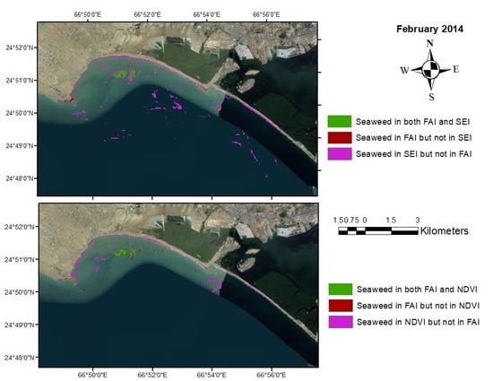
3.3. Validation of Seaweed Enhancing Index (SEI)
For validation purposes, binary images of all indices of the same dates were overlaid. The accuracy of NDVI and SEI was assessed by matching their spatial extent of seaweed cover with FAI enhanced seaweed area (Figure 7). The raster calculator in ArcMap was used to create new images combining FAI separately with NDVI and SEI. The new images had three distinct area classes: (1) Seaweed in both FAI and SEI (NDVI), (2) seaweed in FAI but not in SEI (NDVI), and (3) seaweed in SEI (NDVI) but not in FAI. The remaining pixels in these images belonged to a non-seaweed area in FAI and SEI (NDVI). The pixels overlapping in an index and FAI as seaweed pixels indicated the accuracy of that index. A summary of areas in three classes mentioned here for both SEI and NDVI is given in Table 5. This information will tell the accuracy of SEI and NDVI conforming to FAI, which was being used as the reference index in the study.
4. Discussion
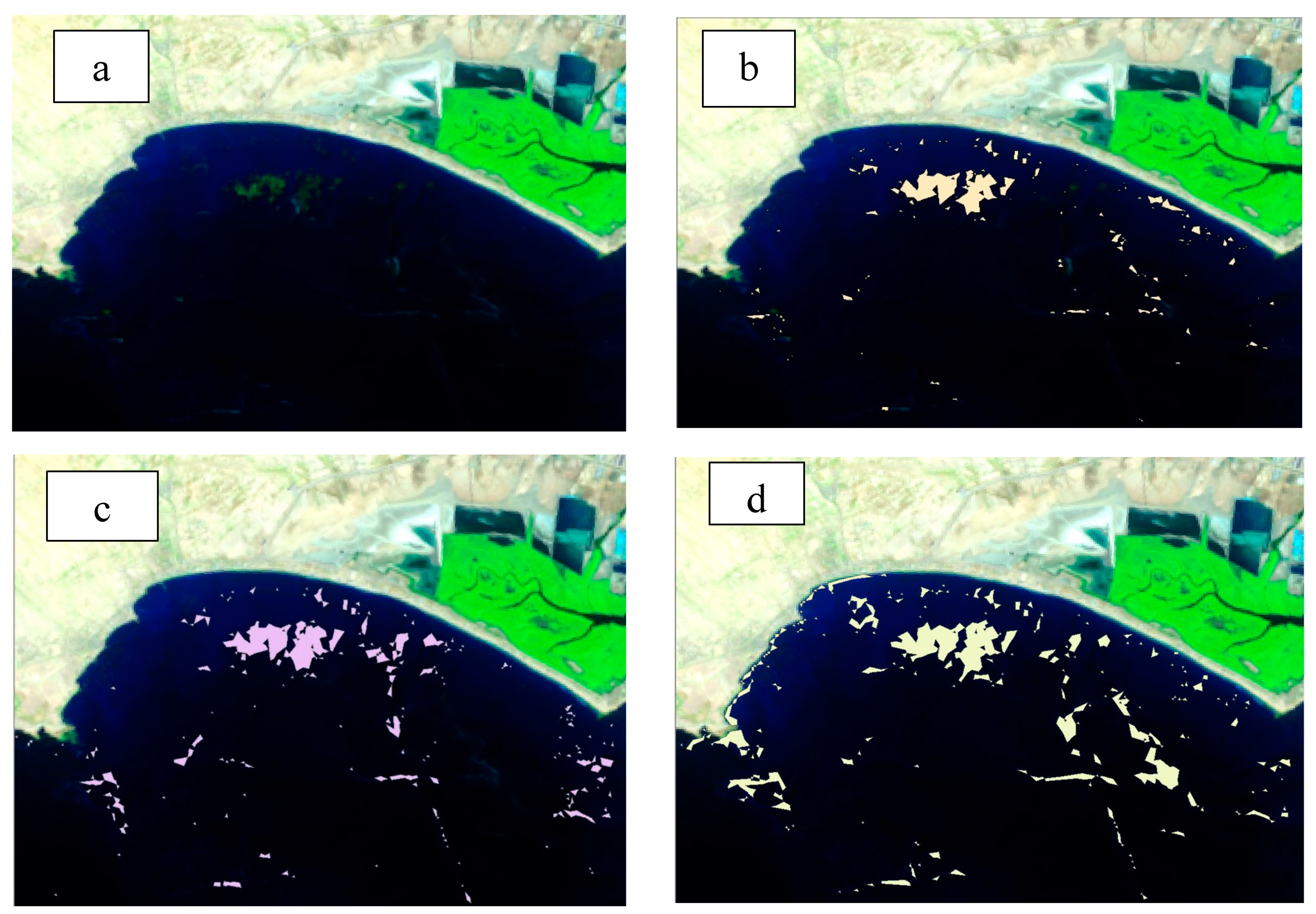
The newly developed seaweed enhancing index (SEI), enhanced larger areas of seaweed resources as compared to NDVI and FAI, as shown in (Figure 5). The results showed that NDVI extracted fewer seaweed areas as compared to FAI and SEI. In NDVI, big patches of seaweed were enhanced, but it failed to enhance the attached seaweed (Figure 8). Besides NDVI, FAI also could not map attached seaweeds on rocky areas very well. However, in SEI seaweeds attached on rocks were enhanced, but also got mixed with some non-seaweed rocky pixels.
Seaweed areas enhanced by SEI and NDVI overlapping FAI seaweed area as the percentages of total FAI seaweed area (A/(A + B) × 100) are presented in Table 6. The SEI images of January 2016, February 2018, and March 2018 enhanced less than 50 percent of the corresponding FAI total seaweed areas. However, on these dates, the NDVI performed very well, matching more than 95 percent of FAI seaweed coverage. Except for these three years, the performance of SEI in the remaining six images was either similar to NDVI or even better than NDVI. On January 2018, SEI enhanced 99 percent of FAI seaweed cover. Overall, the seaweed area not covered by FAI was greater in SEI than NDVI in almost all images, which needs to be further explored in future studies by collecting extensive field information to validate SEI mapped additional area beyond the extent of FAI seaweed cover. Based on these results, in the majority of the satellite temporal images selected for this study, the performance of the newly proposed index—SEI—was found either better than or similar to NDVI. Except one, almost in all cases, the index area as seaweed not covered by FAI was greater in SEI than NDVI. These locations need to be validated through field collected data where SEI has mapped seaweed, but FAI has not.
5. Conclusions
In this study, three indices—floating algal index (FAI), normalized difference vegetative index (NDVI), and seaweed enhancing index (SEI)—were applied on Landsat 8 temporal images to extract seaweed patches along the Karachi Coast. Analyzing satellite mapped data, the following trends were observed:
- All three indices enhanced seaweed at the verified field collected GPS locations in all temporal images, which employed that the GPS points were at the permanent (seasonal) seaweed sites.
- Area estimation of seaweed resources of three indices showed variations. Overall, SEI extracted seaweed area was more than both NDVI and FAI, which was probably due to SEI capability of enhancing rocked attached patches and overestimation of rocked area. Another reason may be the possibility of SEI enhancing the submerged aquatic vegetation, which has low SWIR reflectance values [23]. However, this needs to be investigated, and if this reasoning happens to be correct, then it means that SEI works better in enhancing partially submerged seaweed patches, which other indices fail to do.
- NDVI and FAI failed to enhance rock attached seaweed pixels.
- The performance of SEI was found either better than or similar to NDVI based on percent seaweed area of FAI overlapped by the index.
Seaweed assessment is valuable for many stakeholders, including the fisherman community, policymakers, and food and cosmetics industries. These studies can be beneficial to support coastal resources. Remote sensing techniques have been proved as a valuable tool for monitoring and mapping marine resources. In this study, a new seaweed enhancing index was introduced that had the potential to be used for seaweed mapping. This study also demanded some inquiries regarding SEI capabilities in mapping partially submerged patches. A more detailed study is needed over a longer period to validate this notion. If this hypothesis happens to be true, it will open the possibility of detecting seaweed locations more precisely with SEI.
Author Contributions
Conceptualization, M.D.S. and M.A.; methodology, M.D.S. and A.Z.Z.; software, NA; validation, M.D.S. and A.Z.Z.; formal analysis, M.D.S. ; investigation, M.D.S. and A.Z.Z.; resources, A.Z.Z.; data curation, M.D.S. and M.A.; writing—original draft preparation, M.D.S.; writing—A.Z.Z.; visualization, M.D.S.; supervision, A.Z.Z.; project administration, M.D.S. and M.A.; funding acquisition, A.Z.Z., M.D.S.
Funding
This research was partially funded by Mangroves for the Future (MFF) of IUCN, grant number, NA. The APC was waived.
Acknowledgments
We, the authors, are grateful to the Centre of Excellence in Marine Biology, the University of Karachi for arranging collaborative field survey. We would also like to knowledge Rafey Ali, a research specialist at The Aga Khan University, for his valuable assistance in this research.
Conflicts of Interest
The authors declare no conflict of interest. The funders had no role in the design of the study; in the collection, analyses, or interpretation of data; in the writing of the manuscript, or in the decision to publish the results.
References
- Magg, W. Seaweed—Types of Seaweed; Te Ara-the Encyclopedia of New Zealand: Wellington, New Zealand, 2006.
- Haq, T.; Khan, F.A.; Begum, R.; Munshi, A.B. Bioconversion of drifted seaweed biomass into organic compost collected from the Karachi coast. Pak. J. Bot. 2011, 43, 3049–3051. [Google Scholar]
- Choi, C.G.; Takeuchi, Y.; Terawaki, T.; Serisawa, Y.; Ohno, M.; Sohn, C.H. Ecology of seaweed beds on two types of an artificial reef. J. Appl. Phycol. 2002, 14, 343–349. [Google Scholar] [CrossRef]
- Okuda, K. The Coastal Environment and Seaweed-Bed Ecology in Japan. Kuroshio Sci. 2008, 2, 15–20. [Google Scholar]
- Valderrama, D. Social and Economic Dimensions of Seaweed Farming: A Global Review. In Proceedings of the 16th International institute of fisheries economics and trade (IIFET), Dar es Salaam, Tanzania, 16–20 July 2012. [Google Scholar]
- Capuzzo, E.; McKie, T. Seaweed in the UK and Abroad—Status, Products, Limitations, Gaps, and Cefas Role; Centre for Environment, Fisheries & Aquaculture Science (Cefas): Suffolk, UK, 2016.
- Samee, H.; Li, Z.X.; Lin, H.; Khalid, J.; Guo, Y.C. Anti-allergic effects of ethanol extract from brown seaweeds. J. Zhejiang Univ. Sci. B 2009, 10, 147–153. [Google Scholar] [CrossRef] [PubMed]
- Pickrill, R.A.; Kostylev, V.E. Habitat Mapping and National Seafloor Mapping Strategies in Canada. Geol. Assoc. Canada 2007, 47, 449–462. [Google Scholar]
- Eakin, C.M.; Nim, C.J.; Brainard, R.E.; Aubrecht, C.; Elvidge, C.; Gledhill, D.K.; Muller-Karger, F.; Mumby, P.J.; Skirving, W.J.; Strong, A.E.; et al. Monitoring coral reefs from space. Oceanography 2010, 23, 118–133. [Google Scholar] [CrossRef]
- Hyun, J.C.; Deepak, M.; John, W. Remote Sensing of Submerged Aquatic Vegetation. In Remote Sensing—Applications; IntechOpen: London, UK, 2012. [Google Scholar] [Green Version]
- He, M.X.; Liu, J.; Yu, F.; Li, D.; Hu, C. Monitoring green tides in Chinese marginal seas. In Handbook of Satellite Remote Sensing Image Interpretation: Applications for Marine Living resources conservation and management; Morales, J., Stuart, V., Platt, T., Sathyendranath, S., Eds.; EU PRESPO and IOCCG: Dartmouth, NS, Canada, 2011; pp. 111–124. [Google Scholar]
- Gower, J.; Hu, C.; Borstad, G.; King, S. Ocean color satellites show extensive lines of floating Sargassum in the Gulf of Mexico. IEEE Trans. Geosci. Remote Sens. 2006, 44, 3619–3625. [Google Scholar] [CrossRef]
- Gower, J.; King, S.; Goncalves, P. Global monitoring of plankton blooms using MERIS MCI. Int. J. Remote Sens. 2008, 29, 6209–6216. [Google Scholar] [CrossRef]
- Ko, B.; Kim, H.; Nam, J. Classification of potential water bodies using Landsat 8 OLI and a combination of two boosted random forest classifiers. Sensors 2015, 15, 13763–13777. [Google Scholar] [CrossRef] [PubMed]
- Hu, C. A novel ocean color index to detect floating algae in the global oceans. Remote Sens. Environ. 2009, 113, 2118–2129. [Google Scholar] [CrossRef]
- Hu, C.; He, M. Origin and offshore extent of floating algae in Olympic sailing area. Eos Trans. Am. Geophys. Union 2008, 89, 302. [Google Scholar] [CrossRef]
- El-Alem, A.; Chokmani, K.; Laurion, I.; El-Adlouni, S.E. Comparative analysis of four models to estimate chlorophyll-a concentration in case-2 waters using MODerate resolution imaging spectroradiometer (MODIS) imagery. Remote Sens. 2012, 4, 2373–2400. [Google Scholar] [CrossRef]
- Campbell, J.B.; Wynne, R.H. Introduction to Remote Sensing; Guilford Press: New York, NY, USA, 2011. [Google Scholar]
- Cho, H.J.; Lu, D. A water-depth correction algorithm for submerged vegetation spectra. Remote Sens. Lett. 2010, 1, 29–35. [Google Scholar] [CrossRef]
- Lubin, D.; Li, W.; Dustan, P.; Mazel, C.H.; Stamnes, K. Spectral signatures of coral reefs: Features from space. Remote Sens. Environ. 2001, 75, 127–137. [Google Scholar] [CrossRef]
- Ali, A.; Malik, S.; Zaidi, A.Z.; Ahmad, N.; Shafique, S.; Aftab, M.N.; Aisha, K. Standing Stock Of Seaweeds In Submerged Habitats Along The Karachi Coast, Pakistan: An Alternative Source Of Livelihood For Coastal Communities. Pak. J. Bot. 2019, 51, 5. [Google Scholar] [CrossRef]
- Dierssen, H.M.; Zimmerman, R.C.; Bissett, P.J. The Red Edge: Exploring high near-infrared reflectance of phytoplankton and submerged macrophytes and implications for aquatic remote sensing. In AGU Spring Meeting Abstracts; American Geophysical Union (AGU): Washington, DC, USA, 2007. [Google Scholar]
- Hestir, E.L. Trends in Estuarine Water Quality and Submerged Aquatic Vegetation Invasion; University of California: Davis, CA, USA, 2010. [Google Scholar]
Figure 1.
Study area: Hawks Bay beach along the Sindh Coast with GPS points on the seaweed patches.

Figure 2.
Spectral response of seaweed, mangrove, and water. On the x-axis Landsat 8 bands are shown and on the y-axis top of atmosphere (ToA) reflectance values are presented.
Figure 2.
Spectral response of seaweed, mangrove, and water. On the x-axis Landsat 8 bands are shown and on the y-axis top of atmosphere (ToA) reflectance values are presented.
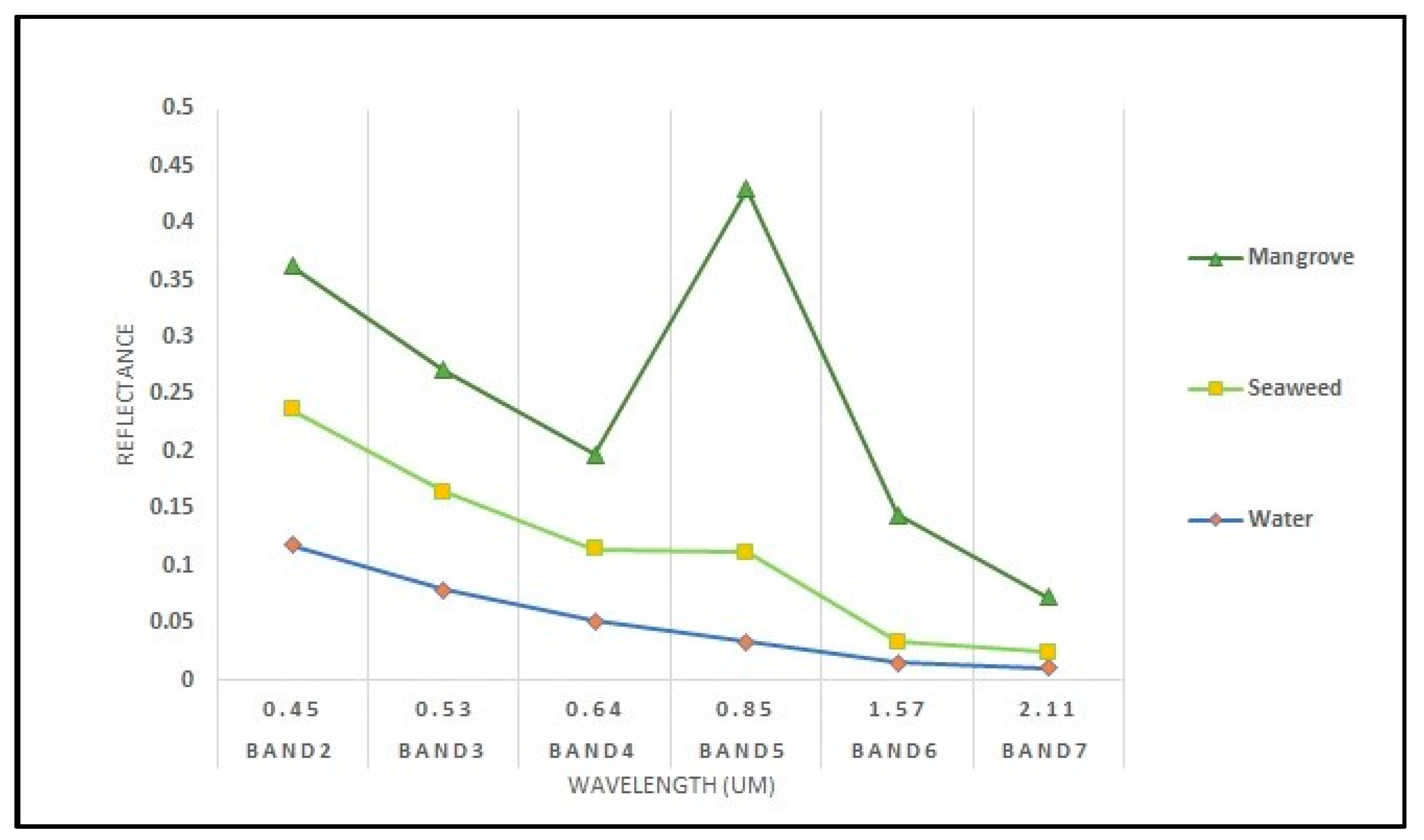
Figure 3.
This figure shows the floating algae index (FAI) with values ranging from −0.51 to 0.53. The red oval highlights the seaweed patches (26 February 2014).
Figure 3.
This figure shows the floating algae index (FAI) with values ranging from −0.51 to 0.53. The red oval highlights the seaweed patches (26 February 2014).
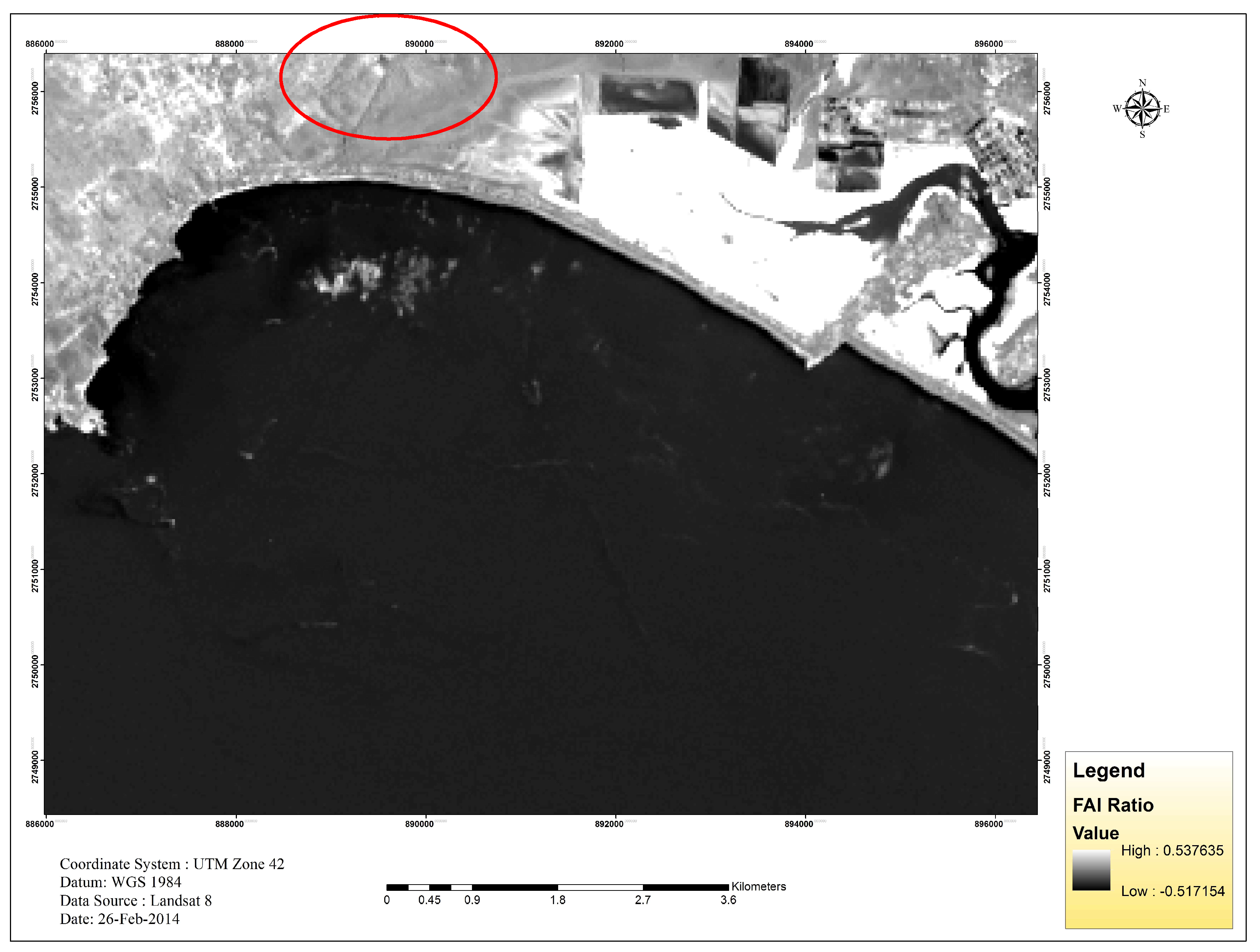
Figure 4.
This figure shows NDVI with values ranging from –0.145 to 0.372. The red oval highlights the seaweed patches (26 February 2014).
Figure 4.
This figure shows NDVI with values ranging from –0.145 to 0.372. The red oval highlights the seaweed patches (26 February 2014).
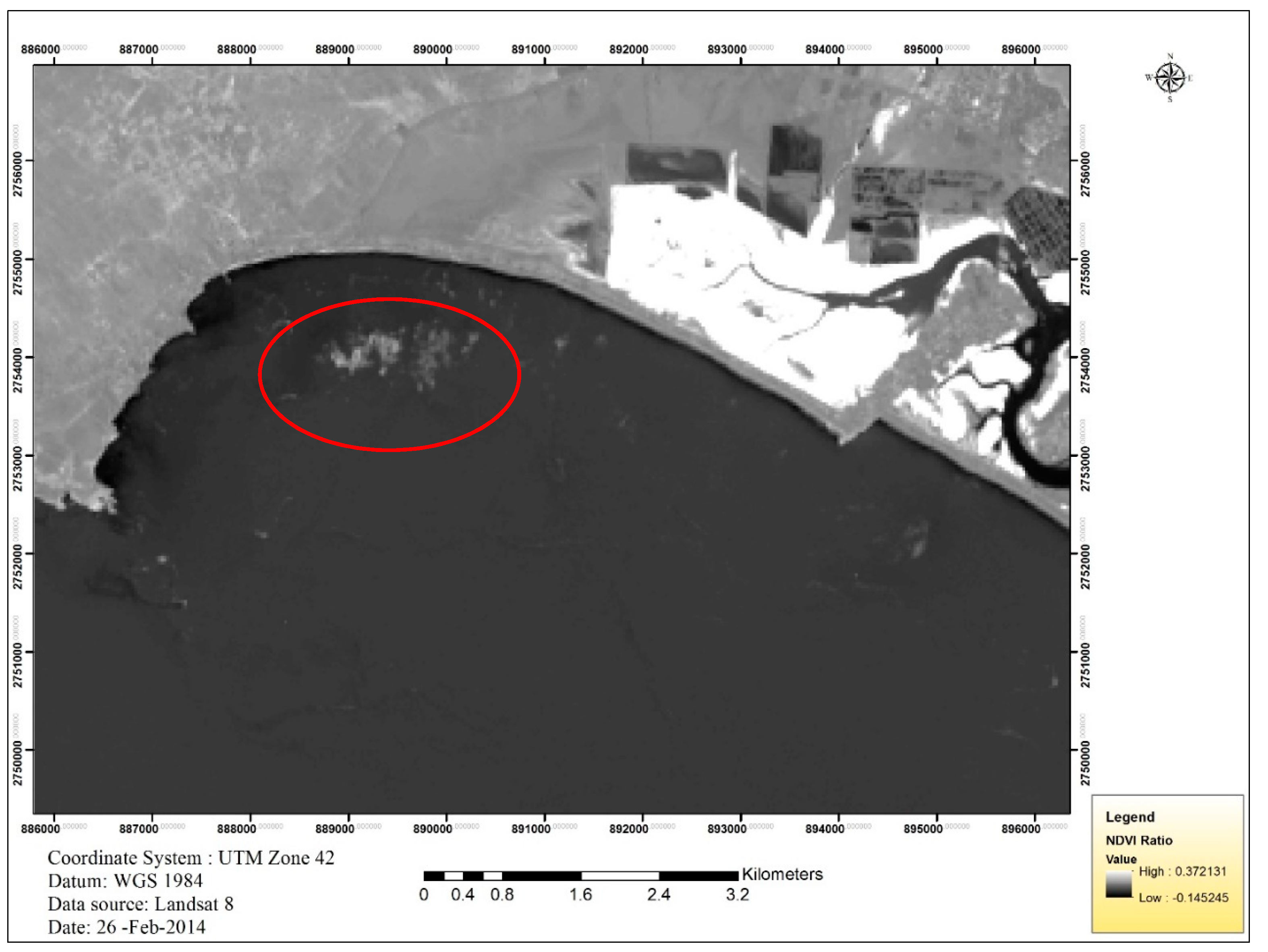
Figure 5.
This figure shows the seaweed enhancing index (SEI) with values ranging from −0.85 to 0.307. The red oval highlights the seaweed patches (26 February 2014).
Figure 5.
This figure shows the seaweed enhancing index (SEI) with values ranging from −0.85 to 0.307. The red oval highlights the seaweed patches (26 February 2014).
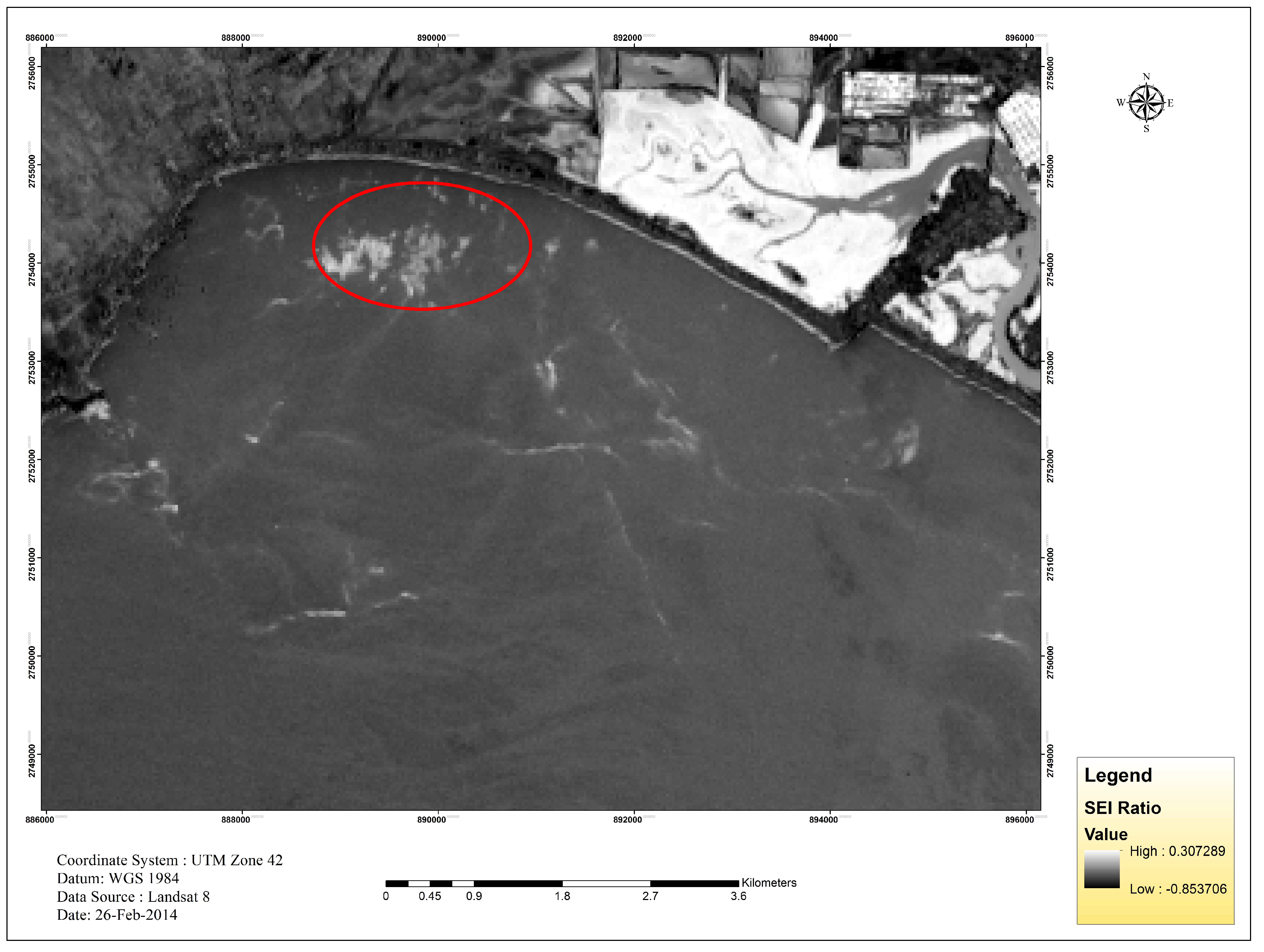
Figure 6.
Graph showing estimated areas in all indices.

Figure 7.
This figure compares seaweed extraction of SEI and NDVI with FAI.
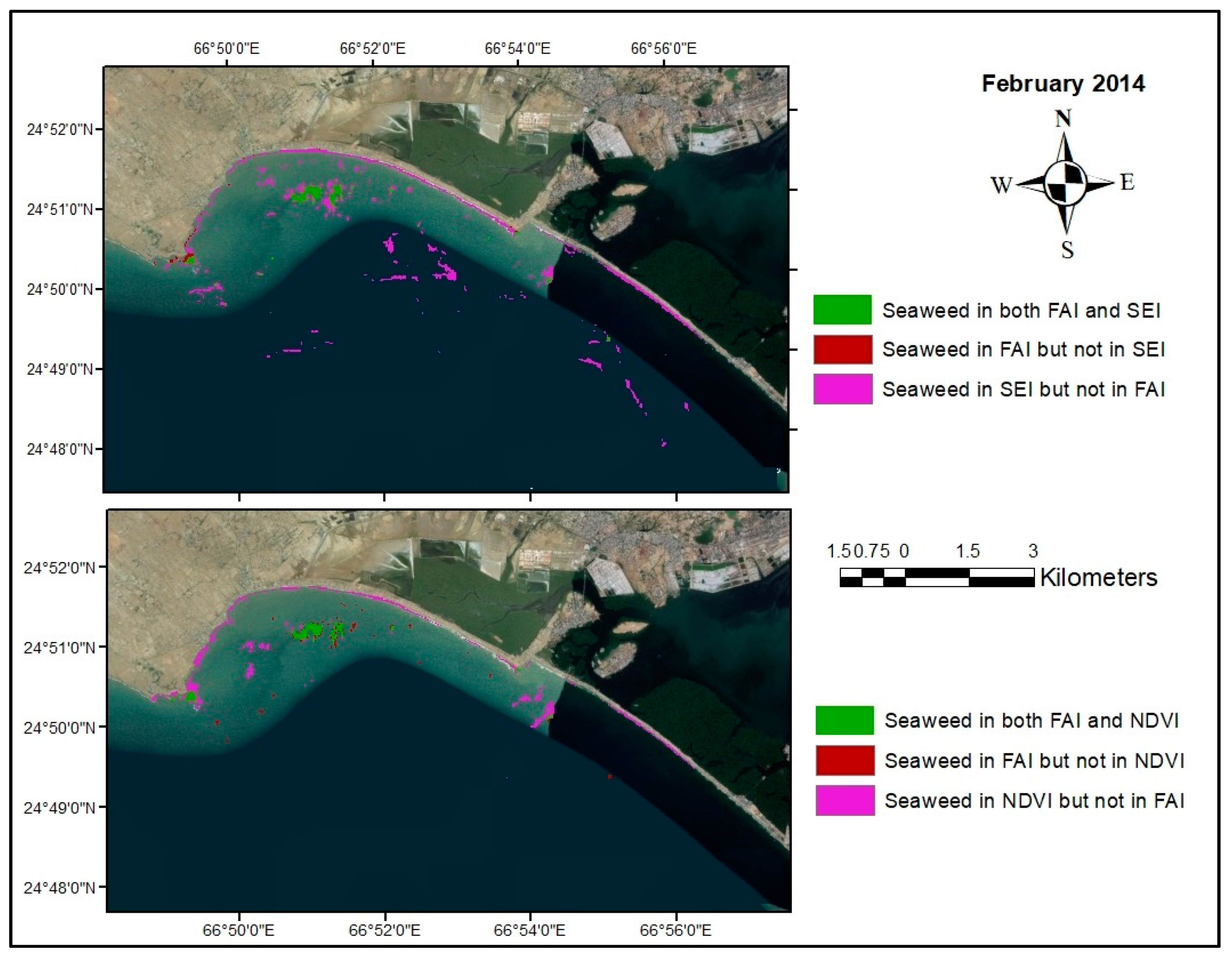
Figure 8.
Seaweed extracted class overlay on Landsat images: (a) False color composite image, (b) NDVI, (c) FAI, and (d) SEI.
Figure 8.
Seaweed extracted class overlay on Landsat images: (a) False color composite image, (b) NDVI, (c) FAI, and (d) SEI.


Table 1.
Floating algae index (FAI) values.
| Class | Pixel Value Range |
|---|---|
| Water | −0.510 to −0.008 |
| Seaweed | 0.008 to 0.130 |
| Mangrove | 0.130 to 0.530 |
Table 2.
Normalized difference vegetation index (NDVI) values.
| Class | Pixel Value Range |
|---|---|
| Water | −0.145 to −0.044 |
| Seaweed | −0.044 to 0.121 |
| Mangrove | 0.159 to 0.372 |
Table 3.
SEI index values.
| Class | Pixel Value Range |
|---|---|
| Water | −0.85 to 0.08 |
| Seaweed | 0.08 to 0.24 |
| Mangrove | 0.24 to 0.307 |
Table 4.
Seaweed area estimation (years 2014, 2016, and 2018).
| Landsat 8 Image Date and Month | Indices | Area Estimation (km2) |
|---|---|---|
| 25 January 2014 | NDVI | 1.78 |
| FAI | 1.91 | |
| SEI | 1.93 | |
| 19 February 2014 | NDVI | 0.98 |
| FAI | 1.97 | |
| SEI | 2.1 | |
| 7 March 2014 | NDVI | 0.594 |
| FAI | 0.75 | |
| SEI | 0.79 | |
| 24 January 2016 | NDVI | 0.59 |
| FAI | 0.63 | |
| SEI | 0.65 | |
| 9 February 2016 | NDVI | 0.7 |
| FAI | 1.1 | |
| SEI | 1.54 | |
| 3 March 2016 | NDVI | 0.908 |
| FAI | 1.8 | |
| SEI | 1.95 | |
| 21 February 2018 | NDVI | 0.30 |
| FAI | 0.34 | |
| SEI | 0.42 | |
| 9 March 2018 | NDVI | 0.190 |
| FAI | 0.32 | |
| SEI | 0.43 |
Table 5.
Areas in km2.
| For NDVI | For SEI | For NDVI | For SEI | ||
|---|---|---|---|---|---|
| Jan 2014 | March 2016 | ||||
| A | 1.3932 | 1.2294 | A | 0.387 | 0.4077 |
| B | 0.2583 | 0.4212 | B | 0.2475 | 0.2268 |
| C | 0.0027 | 0.6498 | C | 0.0009 | 0.7659 |
| Feb 2014 | Jan 2018 | ||||
| A | 0.3501 | 0.4122 | A | 2.7045 | 4.0689 |
| B | 0.1125 | 0.0504 | B | 1.4148 | 0.0504 |
| C | 0.7821 | 1.5129 | C | 0.4122 | 5.1174 |
| March 2014 | Feb 2018 | ||||
| A | 0.4743 | 0.3942 | A | 0.522 | 0.1161 |
| B | 0.0585 | 0.1386 | B | 0.0108 | 0.4167 |
| C | 0.666 | 0.7821 | C | 0.0594 | 0.3519 |
| Jan 2016 | March 2018 | ||||
| A | 0.2421 | 0.081 | A | 0.5076 | 0.0765 |
| B | 0 | 0.1611 | B | 0.0252 | 0.4563 |
| C | 2.8197 | 0.1188 | C | 0.0081 | 0.1188 |
| Feb 2016 | |||||
| A | 0.4374 | 0.612 | Seaweed in both FAI and SEI/NDVI | A | |
| B | 0.2232 | 0.0486 | Seaweed in FAI but not in SEI/NDVI | B | |
| C | 0.1593 | 0.1602 | Seaweed in SEI/NDVI but not in FAI | C | |
Table 6.
Comparing NDVI and SEI with FAI.
| Image Date | Jan-14 | Jan-16 | Jan-18 | Feb-14 | Feb-16 | Feb-18 | Mar-14 | Mar-16 | Mar-18 |
|---|---|---|---|---|---|---|---|---|---|
| Total seaweed area in FAI (km2) | 1.6515 | 0.2421 | 4.1193 | 0.4626 | 0.6606 | 0.5328 | 0.5328 | 0.6345 | 0.5328 |
| NDVI (%) | 84.36 | 100.00 | 65.65 | 75.68 | 66.21 | 97.97 | 89.02 | 60.99 | 95.27 |
| SEI (%) | 74.48 | 33.46 | 98.78 | 89.11 | 92.64 | 21.79 | 73.99 | 64.26 | 14.36 |
© 2019 by the authors. Licensee MDPI, Basel, Switzerland. This article is an open access article distributed under the terms and conditions of the Creative Commons Attribution (CC BY) license (http://creativecommons.org/licenses/by/4.0/).
Share and Cite
MDPI and ACS Style
Siddiqui, M.D.; Zaidi, A.Z.; Abdullah, M. Performance Evaluation of Newly Proposed Seaweed Enhancing Index (SEI). Remote Sens. 2019, 11, 1434. https://doi.org/10.3390/rs11121434
AMA Style
Siddiqui MD, Zaidi AZ, Abdullah M. Performance Evaluation of Newly Proposed Seaweed Enhancing Index (SEI). Remote Sensing. 2019; 11(12):1434. https://doi.org/10.3390/rs11121434
Chicago/Turabian StyleSiddiqui, Muhammad Danish, Arjumand Z. Zaidi, and Muhammad Abdullah. 2019. "Performance Evaluation of Newly Proposed Seaweed Enhancing Index (SEI)" Remote Sensing 11, no. 12: 1434. https://doi.org/10.3390/rs11121434
Note that from the first issue of 2016, this journal uses article numbers instead of page numbers. See further details here.