Spectral–Spatial Discriminant Feature Learning for Hyperspectral Image Classification

Abstract

Sparse representation classification (SRC) is being widely applied to target detection in hyperspectral images (HSI). However, due to the problem in HSI that high-dimensional data contain redundant information, SRC methods may fail to achieve high classification performance, even with a large number of spectral bands. Selecting a subset of predictive features in a high-dimensional space is an important and challenging problem for hyperspectral image classification. In this paper, we propose a novel discriminant feature learning (DFL) method, which combines spectral and spatial information into a hypergraph Laplacian. First, a subset of discriminative features is selected, which preserve the spectral structure of data and the inter- and intra-class constraints on labeled training samples. A feature evaluator is obtained by semi-supervised learning with the hypergraph Laplacian. Secondly, the selected features are mapped into a further lower-dimensional eigenspace through a generalized eigendecomposition of the Laplacian matrix. The finally extracted discriminative features are used in a joint sparsity-model algorithm. Experiments conducted with benchmark data sets and different experimental settings show that our proposed method increases classification accuracy and outperforms the state-of-the-art HSI classification methods.

1. Introduction

In recent years, hyperspectral image (HSI) analysis has received an increasing amount of interest among the remote sensing community, such as military investigation, agriculture, mineralogy, surveillance, and chemical imaging. Each pixel in a hyperspectral image is captured from hyperspectral sensors containing hundreds of contiguous spectral channels (termed as bands) over a wide range of the electromagnetic spectrum. This brings target classification advantages when identifying the target of interest in a hyperspectral scene by exploiting the spectral signatures of the materials.

To accurately classify a target, numerous advanced approaches have been proposed for hyperspectral image classification [1,2,3,4,5,6,7,8]. A number of statistical hypothesis testing techniques [9,10,11,12] have also been proposed for target detection in HSI, such as the spectral matched filter (SMF), matched subspace detectors (MSDs) [13], adaptive subspace detectors (ASDs) [12], Reed-CXiaoli (RX) anomaly detector [14,15], kernel RX [16,17], and traditional Gaussian and linear mixture models. In cases where target information exists, these target detection algorithms usually try to match the target’s signature distribution to the suspect pixel and suppress the background. However, these methods are not robust in low contrast and local noise situations, which leads to inaccurate results on target detection. Meanwhile, support vector machines (SVM) [18,19,20,21] are found to be highly effective for supervised hyperspectral classification, where the classifier is trained by solving an optimization function. Recently, sparse representation (SR) algorithms [22,23,24,25,26] have been applied to tackle the HSI task. Chen et al. [27] proposed the pixelwise-based SR technique for HSI target detection. However, this detection technique is performed for each pixel in the test image independently, regardless of the spatial correlation of neighboring pixels. To exploit this crucial interpixel correlation, some additional smoothing terms, such as the Laplacian [28] or total variation [29], were added in the optimization formulation. On a different note, the joint SR [30,31,32] that incorporates interpixel correlation information of neighborhoods was proposed to further improve classification performance.

The abundance of information provided by hyperspectral data can be leveraged to enhance the ability to classify and recognize materials. However, this high dimensionality of hyperspectral data leads to a huge increase in the computational complexity of classification. Moreover, since there is a high likelihood of redundancy between the spectral features, it has a negative impact on classification accuracy. Some features contain less discriminatory information than others, which are not useful for producing a desired learning result, and the limited observations may lead the learning algorithm to overfit to the noise. Therefore, to achieve an excellent classification performance, a dimensionality reduction (DR) [33,34,35,36] procedure is required before training the classifier, which is used to reduce computational complexity and improve classification accuracy. The common dimensionality reduction method can be summarized as feature selection and feature extraction. Feature selection methods [37,38,39,40] attempt to identify a subset of features that contain the fundamental characteristics of the data. The removal of multi-collinearity can improve the interpretation of the data. Most of the feature selection methods are based on feature ranking, which construct and evaluate an objective matrix based on various criteria, such as dependence measures [41,42,43], class separability measures [44,45,46], distance measures, and information measures. Feature extraction methods [47,48,49], such as principal component analysis (PCA) [50], independent component analysis (ICA) [51], non-negative matrix factorization (NMF), locality preserving projection (LPP) [52,53], linear discriminant analysis (LDA) [54], generalized discriminant analysis (GDA), Fisher discriminant analysis (LFDA), canonical correlation analysis (CCA), and local discriminant embedding (LDE), project the high-dimensional data into a low-dimensional feature space, while preserving the discriminative information of different classes.

In addition, extensive work has been done to make full use of the spectral–spatial information in hyperspectral images. For instance, dimensionality reduction methods have been proposed for the integration of spatial and spectral information in hyperspectral feature learning. Thus, the structure of the manifold could be preserved in the resulting features for classification, as evident in methods such as watershed [55], clustering [56], hierarchical segmentation [57], minimum spanning forest [58,59], and probabilistic modeling [60,61,62,63,64,65,66] methods.

Taking these into consideration, we propose a discriminant feature learning scheme for hyperspectral image classification based on sparse representation, which considers the spectral and spatial knowledge to achieve the low-dimensional representations of hyperspectral image data. The proposed method includes two main strategies for reducing features: firstly, it employs the spectral knowledge to select a low-dimensional discriminant subset of spectral features from the original high-dimensional feature set, based on feature score ranking. Secondly, the discriminant subset is fused and projected onto a Laplacian eigenspace to further reduce dimensionality and preserve properties of the low dimensional manifold by integrating both the spatial and spectral knowledge in a hypergraph. Finally, the simultaneous joint sparse representation algorithm is exploited to obtain the representation of the pixels. The recovered sparse errors are used for determining the label of the pixels. The main contribution of this work is summarized as follows: (1) a new feature evaluator is obtained based on a graphical model with semi-supervised learning and used for the selection of discriminative hyperspectral bands; (2) low-dimensional spectral–spatial features are acquired through a generalized eigen decomposition of a Laplacian matrix of the selected bands; and (3) the learned low-dimensional features improve the performance of classification due to the dimensionality and redundancy reduction.

The remainder of this paper is organized as follows. Section 2 presents a brief recapitulation of the proposed evaluator for the discriminant feature learning. Section 3 elaborates our proposed hyperspectral image classification framework using discriminant feature learning and the simultaneous joint sparsity classification. Section 4 contains experimental work and Section 5 discusses the implementation of our method, followed by the conclusion (Section 6).

2. Evaluator for Discriminant Feature Learning

The first step in feature learning is to search for the best subset of attributes in a dataset. An effective feature evaluator is crucial for a feature selection algorithm. In this paper, we propose to evaluate features based on a semi-supervised graph-based Laplacian model.

Our feature evaluator is based on the graph theory. We briefly review a precise notion for a graph that we work with, in which a hypergraph $G=\left(V,E\right)$ consists of vertices (nodes) $V$ and edges $E$. An edge $e$, spanning two nodes $v_i$ and $v_j$, is denoted by $e_{ij}$. A graph assigns a value to each edge, called a weight.

Notate a hyperspectral training dataset from $C$ classes as $X^{train}={\left\{\left(x_i,y_i\right)\right\}}_{i=1}^{N^{train}}$, where $x_i\in {ℝ}^d$ is a training sample and $y_i\in \{1,2,\dots ,C\}$ is the class label of the sample. Based on the weighted connection graph, the estimation of the probabilities of the samples belonging to a class can be solved by minimizing the following energy function:

$$E=\frac{1}{2}{\displaystyle \sum _{i,j=1}^{N^{train}}{W}_{ij}^{}{\left(p_i^{}-p_j^{}\right)}^2}=p^T{L}^{}p,$$

(1)

where $p_i$ denotes the probability of node $i$, $W$ and $L$ denote the adjacency matrix and Laplacian matrix of a graph.

Our evaluator for discriminant feature learning consists of the following steps:

Step 1 Building a Laplacian hypergraph of hyperspectral data

To preserve the spectral domain similarity and diversity information in the case of limited training samples, we put an edge between nodes $v_i$ and $v_j$ in the following two cases:

Inter-class adjacency connection: $x_i$ and $x_j$ are from the same class, i.e., $y_i=y_j$;

Intra-class adjacency connection: $x_i$ and $x_j$ are from the different class, i.e., $y_i\ne y_j$, but they are mutually in the $\kappa$ nearest neighbors of each other in the original hyperspectral space.

The edge weight is defined by:

$$w_{ij}^{}=\exp \left(-\beta {\Vert x_i^{}-x_j^{}\Vert }^2\right),$$

(2)

where $\beta \in \left[0,1\right]$ is the free heat kernel parameter. We have found it useful to normalize the square spectral similarity ${\Vert x_i^{}-x_j^{}\Vert }^2\forall e_{ij}\in E$ before the application of Equation (2). The corresponding affinity matrix $W$ is used to generate the graph Laplacian matrix $L$. The Laplacian matrix is defined as:

$$L=D-W,$$

(3)

where $D$ is the degree matrix, in which $D_{ii}={\displaystyle \sum _j{W}_{ij}^{}}$ is the node degree for all edges $e_{ij}$ incident on $v_i$. The Laplacian matrix $L$ naturally incorporates the intrinsic spectral knowledge into the hypergraph. It covers all the possible intra-classes and inter-classes defined on the possible feature subset, while measuring the goodness of the classes. Meanwhile, it preserves the data diversity, and overcomes the singularity in the case of limited training samples.

Step 2 Semi-supervised classification based on the Laplacian model

Partition all training sample nodes into two sets: the labeled nodes $V_M$ and unlabeled validation nodes $V_U$. Therefore, the energy function in Equation (1) can be reformulated as follows:

$$\begin{array}{l}E=[{\left(p_M^{}\right)}_{}^T{\left(p_U^{}\right)}_{}^T]\left[\begin{array}{cc}{L}_M^{}& B\\ B^T& L_U^{}\end{array}\right]\left[\begin{array}{c}{p}_M^{}\\ p_U^{}\end{array}\right]\\ ={\left(p_M^{}\right)}_{}^T{L}_M^{}\left(p_M^{}\right)+{\left(p_U^{}\right)}_{}^T{L}_U^{}\left(p_U^{}\right)+2{\left(p_U^{}\right)}_{}^T{B}^T\left(p_M^{}\right)\end{array},$$

(4)

where $p_M$ and $p_U$ correspond to the probabilities of the labeled and unlabeled validation samples, respectively. Finally, the probabilities of the unlabeled samples $p_U$ can be calculated by the following equation:

$$L_U^{}{p}_U^{}=-{\left(B\right)}^T{p}_M^{}.$$

(5)

Extending the above notion to a set of classes, the solution to the combinatorial problem can be obtained by solving:

$$L_U^{}{P}_U^{}=-B^T{P}_M^{}.$$

(6)

$P_U$ and $P_M$ have $C$ columns each, being $p_U$ and $p_M$, respectively. By assigning each validation sample to the class label for which the greatest probability is calculated, a final classification could be obtained.

$$Class\left(x_U\right)=\underset{ c=1,2,\dots ,C}{\arg \max }{P}_U\left(:,c\right).$$

(7)

Step 3 Evaluating features based on the classification results

Computing the classification accuracy on the unlabeled validation set gives the score on this possible feature subset $X$:

$$Evaluator\left(X\right)=\frac{T{P}_{\left(Y_{}^U, Class\left(X_{}^U\right)\right)}+T{N}_{\left(Y_{}^U, Class\left(X_{}^U\right)\right)}}{nu{m}_U},$$

(8)

where $TP$ and $TN$ are the numbers of true positive and true negative sample in the validation dataset, separately. $TP+TN$ is the total number of correct classifications. $nu{m}_U$ is the number of the unlabeled validation set. This accuracy rate is used as the evaluator score.

3. Proposed Method

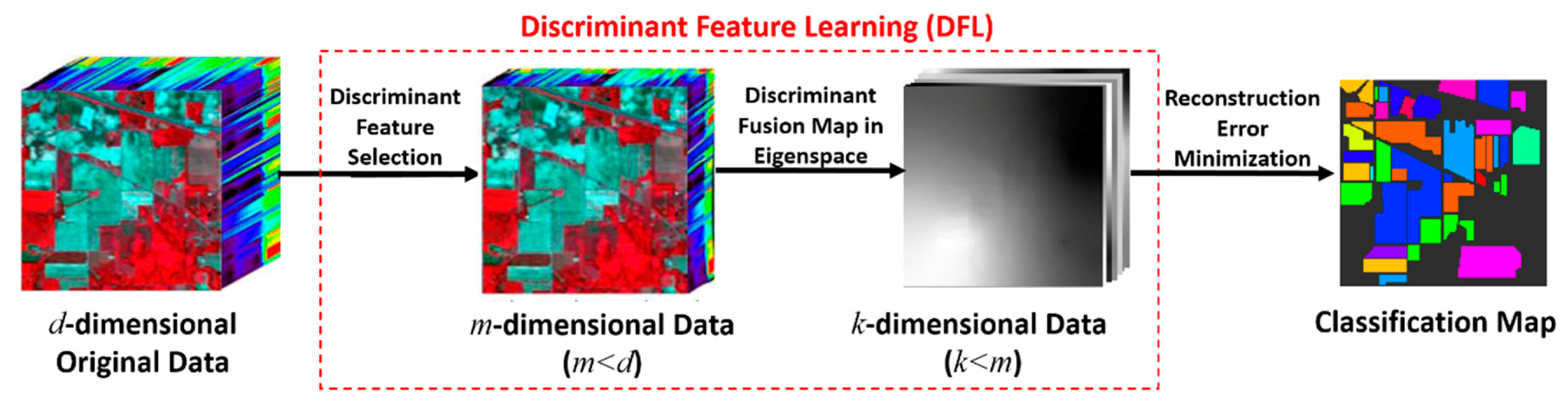
Figure 1 shows the schematic of the proposed discriminant feature learning (DFL) method for hyperspectral image classification. Firstly, a discriminative feature subset was selected based on the proposed evaluator. Furthermore, the selected features were projected onto a low-dimensional Laplacian eigenspace. Then, the simultaneous joint sparsity-based classification algorithm was exploited to obtain the sparse representation of the pixels. Finally, the recovered sparse errors were used for determining the label of the pixels. In the following section, we introduce the discriminant feature learning and the simultaneous joint sparsity-based classification

3.1. Discriminant Feature Learning

As shown in Figure 1, the proposed DFL method firstly selected a subset of discriminative features, which can preserve the intrinsic spectral structure of the unlabeled pixels as well as the inter-class and intra-class constraints defined on the labeled pixels. To incorporate the spatial information, the selected features were mapped into a further lower-dimensional eigenspace through a generalized eigendecomposition of the Laplacian matrix.

3.1.1. Discriminant Feature Selection

Our goal was to reduce the dimensionality of the data by finding a subset of discriminative features that have good classification performance. The simplest algorithm is to test each possible subset of features finding the one which minimizes the error rate. Using a similar principle, we introduced a novel feature selection method in a backward elimination search manner, which ranked the features based on the Laplacian graph model.

The procedure started with the full set of features. At each step, it sequentially removed the least significant feature in the current dataset via the aforementioned Laplacian evaluator criterion. The algorithmic procedure is formally stated in Algorithm 1. (Algorithm 1. Discriminant feature learning via backward elimination.)

Algorithm 1: DFL via Backward Elimination

Input: Training set $X^{train}={\left\{\left(x_i,y_i\right)\right\}}_{i=1}^{N^{train}}, x_i\in {ℝ}^d$    Number of selected bands $m \left(m<d\right)$ Output: Band index set $\mathsf{\Lambda }\in {ℝ}^m$ Initialize: Candidate subset $J_0=X^{train}$, Index set ${\mathsf{\Lambda }}_0=\left\{1,\dots ,d\right\}$, $k=0$ while stopping criterion ($m =d-k$) has not been met do     1. Find the least significant feature with index $j^{-}=\underset{j\in {\mathsf{\Lambda }}_{k-1}}{\arg \max } Evaluator\left(J_{k-1}-x_j\right)$     2. Update index set ${\mathsf{\Lambda }}_k={\mathsf{\Lambda }}_{k-1}-\left\{j^{-}\right\}$     3. Update candidate subset $J_k=J_{k-1}-x_{j^{-}}$     4. Update $k=k+1$ end; $\mathsf{\Lambda }={\mathsf{\Lambda }}_k$

The spectral bands selected by the backward elimination search strategy were optimal in terms of classification performance. In addition, the selected discriminative feature subset can preserve the inter- and intra-class variance in the data due to the semi-supervised classification in the evaluator.

However, this spectral selection method does not consider the spatial information of the hyperspectral data.

3.1.2. Discriminant Feature Fusion

To integrate the underlying spatial structure information into the classification of a hyperspectral image in the selected discriminant feature space, the image was considered as a hyper-graph, where each pixel was associated with a node and a connectivity structure was imposed. This hyper-graph can model the local geometric structure and a spectral–spatial analysis can be performed on the adjacency matrix of the weighted graph.

Consider a hyper-graph with vertices, each vertex representing a hyper pixel. Let $W_{ij}^{\mathsf{\Lambda }}=\exp \left(-\beta {\Vert x_i^{\mathsf{\Lambda }}-x_j^{\mathsf{\Lambda }}\Vert }^2\right)$ be the weight of the edge between adjacent pixels $i$ and $j$ in a small neighborhood, where $\mathsf{\Lambda }$ stands for the discriminative subset indexes corresponding to the original spectral band numbers. To incorporate the spatial information, we fused the selected discriminant features into a new low-dimensional feature space so that neighboring pixels stayed as close together as possible. The new features $f$ can be obtained through minimizing the following objective function [47]:

$${\displaystyle \sum _{i,j=1}^N{\left(f_i^{}-f_j^{}\right)}^2}{W}_{ij}^{\mathsf{\Lambda }}.$$

(9)

The objective function incorporates local spatial information through the adjacency relations of neighboring pixels. In addition, it preserves spectral information by ensuring that if $x_i^{\mathsf{\Lambda }}$ and $x_j^{\mathsf{\Lambda }}$ are close then $f_i$ and $f_j$ are close as well. With some simple algebraic formulations, we have:

$$\begin{array}{ll}{\displaystyle \sum _{i,j=1}^N{\left(f_i^{}-f_j^{}\right)}^2}{W}_{ij}^{\mathsf{\Lambda }}& = {\displaystyle \sum _{i=1}^N{f}_i^T{D}_{ii}^{\mathsf{\Lambda }}{f}_i^{}}+{\displaystyle \sum _{j=1}^N{f}_j^T{D}_{ii}^{\mathsf{\Lambda }}{f}_j^{}}-2{\displaystyle \sum _{i,j=1}^N{f}_i^T}{W}_{ij}^{\mathsf{\Lambda }}{f}_i^{}\\ & =2f^T{L}^{\mathsf{\Lambda }}f\end{array},$$

(10)

where $D^{\mathsf{\Lambda }}$ is the degree matrix and $L^{\mathsf{\Lambda }}$ is the Laplacian matrix in the discriminative feature subset. Finally, the solution to minimizing Equation (10) is:

$$f^{\ast }={\displaystyle \underset{f^T{D}^{\mathsf{\Lambda }}f=1}{\arg \min }} f^T{L}^{\mathsf{\Lambda }}f=\arg \min \frac{f^T{L}^{\mathsf{\Lambda }}f}{f^T{D}^{\mathsf{\Lambda }}f}.$$

(11)

The optimal discriminant feature fusion map $f^{*}$ can be obtained by solving the following generalized eigen problem:

$$L^{\mathsf{\Lambda }}f=\lambda D^{\mathsf{\Lambda }}f.$$

(12)

From the graph partitioning perspective, our method tried to find the optimal cut of the Laplacian graph using the generalized eigendecomposition. $f$ reflects the eigenvector of the above generalized eigenvalue problem with respect to the smallest $k$ eigenvalue and the $k$ ($k<m<d$) is the intrinsic dimensionality of the data in eigenspace. As a result, the final discriminative features $f\in {ℝ}^{k\times N}$ were the eigenvectors associated with the smallest eigenvalues, which were directly used for the sparsity-based classification.

3.2. Simultaneous Joint Sparsity-Based Classification

As described in last section, the low $k$-dimensional discriminative feature $f=\left[f_{{}^1},f_2,\dots ,f_{{}^N}\right]\in {ℝ}^{k\times N}$ could be obtained from the original high $d$-dimensional hyperspectral data. Furthermore, the corresponding k-dimensional discriminative training set $A={\left\{\left(f_i,y_i\right)\right\}}_{i=1}^{N^{train}}s$ could be archived, where $y_i\in \{1,2,\dots ,C\}$ and $C$ is the number of distinct classes. Let $z=f_i$ be a k-dimensional unknown test sample in the discriminant feature fusion map. Based on a pixelwise sparsity model, $z$ can be written by:

$$z=A^1{\mathsf{\alpha }}^1+A^2{\mathsf{\alpha }}^2+\dots +A^C{\mathsf{\alpha }}^C =\underset{A}{\underbrace{\left[A^1,\dots ,A^C\right]}}\left[\begin{array}{c}{\mathsf{\alpha }}^1\\ ⋮\\ {\mathsf{\alpha }}^C\end{array}\right]=A\mathsf{\alpha },$$

(13)

where $A={\left\{A^c\right\}}_{c=1,2,\dots ,C}^{}$ is a structured dictionary consisting of training samples from all classes, and $A^c$ is a class subdictionary whose columns are the training samples in the $c$-th class; $\mathsf{\alpha }$ is a sparse vector formed by concatenating the sparse vectors ${\left\{{\mathsf{\alpha }}^c\right\}}_{c=1,2,\dots ,C}^{}$. However, a pixelwise sparsity model for classification in hyperspectral data focuses on analyzing the data without incorporating information on the spatially adjacent data.

To incorporate the contextual information within the neighboring pixels into the pixelwise sparsity model, we exploited the simultaneous sparsity model as our classifier. In this work, HSI pixels in a small spatial neighborhood were approximated by a sparse linear combination of a few common atoms from a given structured dictionary, but these atoms were weighted with a different set of coefficients for each pixel.

Consider a small neighborhood $N_{\epsilon }$ consisting of $T$ pixels (four or eight neighbors), represented by a matrix $Z=\left[\begin{array}{cccc}{z}_1& z_2& \dots & z_T\end{array}\right]$, where the columns ${\left\{z_t\right\}}_{t=1,\dots ,T}$ are pixels in a spatial neighborhood. The simultaneous sparsity model represents $Z$ by:

$$\begin{array}{l}Z=\left[\begin{array}{cccc}{z}_1& z_2& \cdots & z_T\end{array}\right]=\left[\begin{array}{cccc}A{\mathsf{\alpha }}_1& A{\mathsf{\alpha }}_2& \cdots & A{\mathsf{\alpha }}_T\end{array}\right]\\ =A\left[\begin{array}{cccc}{\mathsf{\alpha }}_1& {\mathsf{\alpha }}_2& \cdots & {\mathsf{\alpha }}_T\end{array}\right]=AS\end{array}.$$

(14)

Given the training dictionary $A$, the representation matrix $S$ can be obtained by solving the following optimization problem:

$$\widehat{S}=\arg \min \Vert AS-Z\Vert subject to {\Vert S\Vert }_{row,0}\le K_0.$$

(15)

The class of $Z$ can be determined directly by the characteristics of the recovered sparse vector $\widehat{S}$. The sparse reconstruction error between the test sample and the reconstruction from training samples in the $c$-th class is:

$$r^c\left(Z\right)=\sqrt{{\displaystyle \sum _{i=1}^T{\Vert A^c{\widehat{S}}^c-Z\Vert }_2^2}} c=1,2,\dots ,C,$$

(16)

where ${\widehat{S}}^c$ denotes the portion of the recovered sparse coefficients corresponding to the training samples in the $c$-th class. The class label of the Z is then determined to be the class that yields the minimal total residuals:

$$Class\left(Z\right)=\underset{ c=1,2,\dots ,C}{\arg \min }{r}^c\left(Z\right).$$

(17)

The simultaneous sparsity model was implemented by the simultaneous orthogonal matching pursuit algorithm (SOMP) [30]. In SOMP, the atom that simultaneously yields the best approximation to all of the residual vectors is selected at each iteration.

4. Results

4.1. Data Sets

In order to make a quantitative evaluation for our proposed method, experiments were conducted with benchmark hyperspectral data sets. The proposed algorithm was implemented in a MacOS-based personal computer (Intel@Corei7 2.5 GHz and 16 GB-DRAM). A detailed description of these HSI data was provided in the following.

Indian Pines Data Set: The first hyperspectral image in our experiments was the commonly-used airborne visible/infrared imaging spectrometer (AVIRIS) Indian Pines image. The AVIRIS sensor generates 220 bands across the spectral range from 0.2 to 2.4 $\mathsf{\mu }\mathrm{m}$. In the experiments, the number of bands was reduced to 200 by removing 20 water absorption bands. The image has a spatial resolution of 20 m per pixel and a size of 145 × 145 pixels. It contains 16 ground-truth classes, most of which are different types of crops (e.g., corns, soybeans, and wheat).

Salinas Data Set: The second hyperspectral image used in our experiments, Salinas image, was also captured by the AVIRIS sensor at Salinas Valley, California. This image contains 224 spectral bands of size 512 × 217. It discarded the 20 water absorption bands before classification. The Salinas data set contains 16 classes of interest, which represent vegetables, bare soils, and vineyard fields.

Pavia University Data Set: The third hyperspectral images used in our experiments, University of Pavia, were urban images acquired by the reflective optics system imaging spectrometer (ROSIS). The ROSIS sensor generates 115 spectral bands ranging from 0.43 to 0.86 $\mathsf{\mu }\mathrm{m}$ and has a spatial resolution of 1.3 m per pixel. The University of Pavia image consists of 610 × 340 pixels, each with 103 bands with the 12 noisiest bands removed. Nine ground-truth classes of interests are considered in the Pavia University data set: trees, asphalt, bitumen, gravel, metal sheets, shadow, bricks, meadows, and bare soil.

4.2. Quantitative Validation of the Proposed DFL for HSI Classification

In the proposed method, we used the discriminant feature learning (DFL) method to obtain the significant features for HSI classification. To demonstrate the effectiveness of the proposed feature learning method for a wide range of classifiers, support vector machine (SVM) [18], orthogonal matching pursuit (OMP) based pixelwise SR classifier [27], and simultaneous orthogonal matching pursuit algorithm (SOMP) based simultaneous joint SR classifier [30] were used in this experiment. The choice of these classifiers was motivated by their demonstrated performances in hyperspectral data classification. In the following experiment, the classification results were compared visually and quantitatively for the three classifiers with and without the DFL.

The classification accuracy for each class was measured by the overall accuracy (OA), the average accuracy (AA), and the Kappa coefficient. The overall accuracy was computed by the ratio between correctly classified test samples and the total number of test samples, and the average accuracy is the mean of multiple class accuracies. The Kappa coefficient was computed by weighting the measured accuracies. It incorporated both of the diagonal and off-diagonal entries of the confusion matrix and is a robust measure of the degree of agreement. We randomly chose about 10% of the labeled samples for training and used the remaining 90% for testing. All the experiments were repeated 10 times with different sets of training and test samples and the average results were used as the classification accuracy.

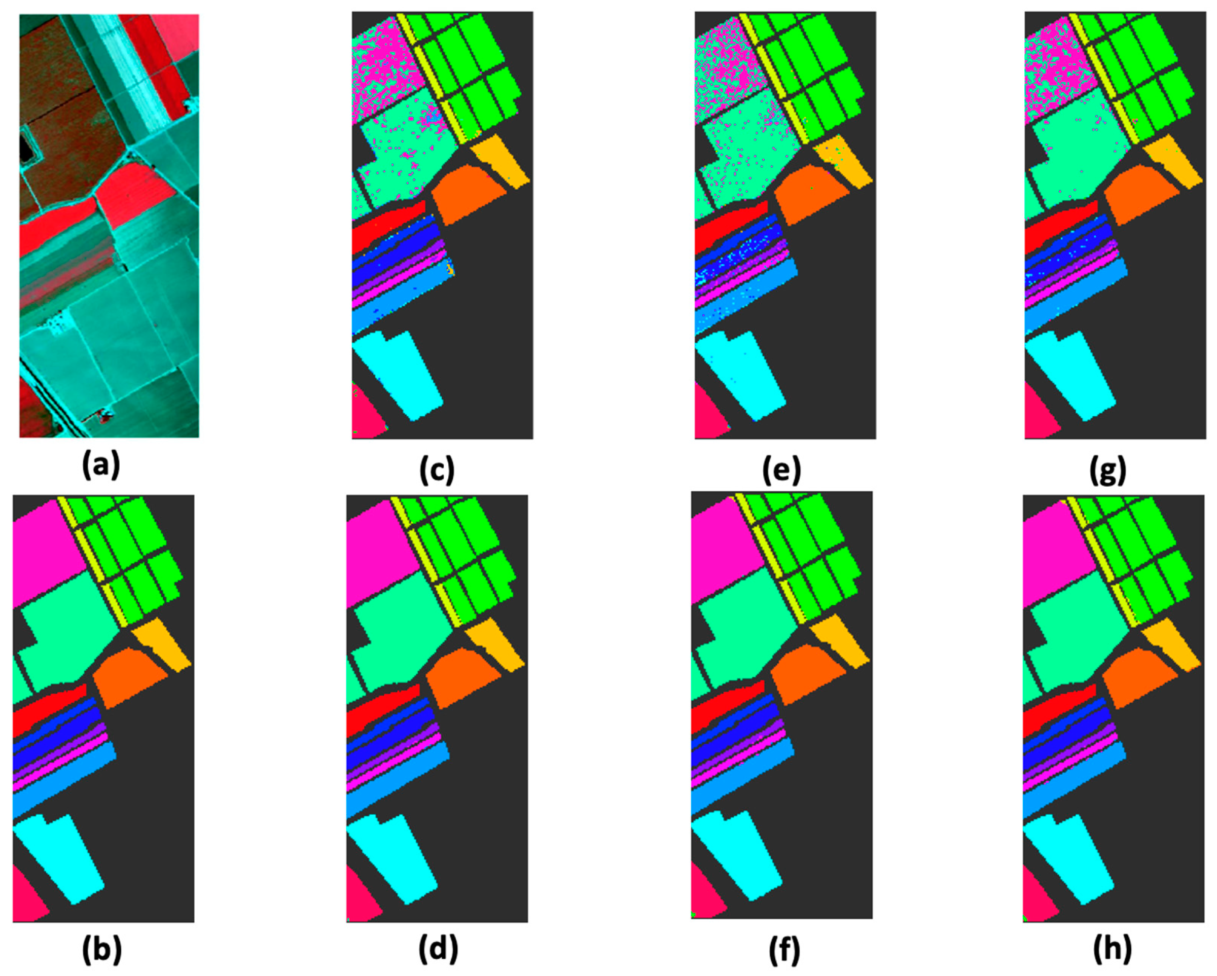
The classification results of the 16 classes in the Indian Pines image are shown in Figure 2. The classification maps of the three classifiers with the DFL method were visually less noisy than their counterparts without the DFL. The quantitative classification accuracies for the Indian Pines data set are summarized in

Table 1. Classification results for Indian Pines data set with/without our proposed discriminant feature learning (DFL). The comparison results of the support vector machine (SVM), SVM with DFL, orthogonal matching pursuit (OMP), OMP with DFL, simultaneous orthogonal matching pursuit algorithm (SOMP) and SOMP with DFL methods.

Class	Training Number	SVM [18]	SVM-DFL	OMP [27]	OMP-DFL	SOMP [30]	SOMP-DFL
Alfalfa	5	1.0	99.0	26.8	100	33.9	99.8
Corn-notill	143	61.5	87.2	52.4	97.6	70.1	97.9
Corn-mintill	83	49.2	98.4	47.9	99.4	59.0	99.4
Corn	24	28.0	99.6	32.1	99.5	51.2	99.5
Grass-pasture	48	80.1	96.9	79.2	97.6	88.9	97.9
Grass-trees	73	97.0	100	91.5	99.9	97.9	99.9
Grass-pasture	3	4.40	99.2	64.4	97.6	81.2	98.8
Hay-windrowed	48	99.7	100	92.4	100	99.5	100
Oats	2	1.1	100	18.3	100	39.4	100
Soybean-notill	97	67.8	89.9	63.8	96.6	67.7	96.9
Soybean-mintill	246	84.5	98.4	69.0	99.2	87.4	99.2
Soybean-clean	59	41.0	97.6	39.5	97.9	61.3	98.2
Wheat	21	96.6	99.9	92.9	99.8	98.4	99.8
Woods	127	97.2	100	88.5	100	97.1	100
Buildings	39	19.0	99.3	38.4	99.5	62.1	99.6
Stone Towers	9	88.8	97.6	84.5	98.3	96.9	97.4
OA		73.0	96.4	66.7	98.8	80.1	98.9
AA		57.3	97.7	61.3	98.9	74.5	99.0
Kappa		68.8	95.9	61.9	98.6	77.0	98.7

. It can be noted that the discriminant features obtained by the proposed DFL method significantly improved the classification accuracy. The improvement was more than 18% and consistent over the three classifiers. Furthermore, the dimensionality reduction capability of the DFL method particularly benefited the classification when the number of training samples was limited. For example, the classes of alfalfa, grass-pasture, and oats in the Indian Pines dataset had five, three, and two training samples, respectively. The improvements of their classifications were the most significant ones.

The classification results of the Salinas image and Pavia University are shown in Figure 3 and Figure 4. The DFL method gained 5-11% accuracy improvement in the Salinas image and 6-11% in the Pavia University image. It can be concluded that the proposed DFL method consistently improved the classification accuracy of the three benchmark datasets for all the three classifiers.

4.3. Comparison with Other Spectral–Spatial HSI Classification Methods

We also compared our method with five state-of-the-art spectral–spatial HSI classification methods-Logistic Regression via Splitting and Augmented Lagrangian (LORSAL) [64], LORSAL with a Multilevel Logistic Prior (LORSAL-MLL) [64], Edge-Preserving Filtering (EPF) [60], Maximizer of the Posterior Marginal by Loopy Belief Propagation (MPM-LBP) [65], and Basic Thresholding Classifier (BTC) [67].

Table 2. Comparison of spectral–spatial hyperspectral images (HSI) classification accuracies the for Indian Pines data set. The results of the Logistic Regression via Splitting and Augmented Lagrangian (LORSAL) [64], LORSAL with a Multilevel Logistic Prior (LORSAL-MLL) [64], Edge-Preserving Filtering (EPF) [60], Maximizer of the Posterior Marginal by Loopy Belief Propagation (MPM-LBP) [65], Basic Thresholding Classifier (BTC) [67] and our proposed SOMP-DFL methods.

Training Sample Number	Metrics	Spectral–Spatial HSI Methods
		LORSAL [64]	EPF [60]	LORSAL-MLL [64]	MPM-LBP [65]	BTC [67]	SOMP-DFL
1%	OA	57.8	66.6	70.1	69.4	66.1	89.4
	AA	53.6	51.6	64.3	64	55.8	91.6
	Kappa	51.4	60.8	65.4	64.6	60.2	88.0
5%	OA	75.0	86.4	89.2	89.3	90.8	97.9
	AA	64.4	70.2	75.9	77.0	76.7	98.3
	Kappa	71.4	84.4	87.6	87.7	89.5	97.6
10%	OA	80.9	92.8	94.2	95.0	96.7	98.9
	AA	72.6	81.8	86.3	88.8	91.9	99.0
	Kappa	78.2	91.8	93.3	94.3	96.2	98.7
15%	OA	83.9	95.1	95.5	96.7	97.7	99.3
	AA	77.1	86.0	90.7	93.4	95.4	99.4
	Kappa	77.1	86.0	90.7	93.4	97.4	99.2
20%	OA	85.5	97.1	96.5	97.5	98.3	99.3
	AA	85.5	97.1	96.5	97.5	96.6	99.4
	Kappa	83.5	96.6	96.0	97.1	98	99.2
25%	OA	86.9	97.6	97.2	98.2	98.5	99.4
	AA	82.2	94.4	95.0	96.0	97.1	99.3
	Kappa	85.0	97.3	96.8	97.9	98.3	99.3
30%	OA	87.9	98.0	97.4	98.5	98.7	99.5
	AA	84.3	95.6	96.1	97.2	98	99.5
	Kappa	86.1	97.8	97.0	98.2	98.5	99.5

shows the OA, AA, and Kappa coefficient (Kappa) of the different spectral-spatial based HSI classification methods for the Indian Pines dataset. In this table, the same training and test sets were used for all the methods, while the LORSAL, LORSAL-MLL, MPM-LBP, EPF, and BTC methods used the default parameters given in [60,64,65,66], respectively. In this case, our proposed DFL with SOMP produced the best classification results. Table 2 also shows the results with different numbers of training samples (1–30% of the reference data). We can see that the classification accuracies of all spectral-spatial algorithms improved with the increase in the number of training samples. The reason for this was that a large number of training samples contained more available information to learn low-dimensional features. The proposed SOMP-DFL method consistently outperformed other methods and the improvement was more significant when a smaller number of labeled training samples were used.

4.4. Comparison with State-Of-The-Art HSI Dimensionality Reduction Methods

In this section, the experiments were conducted with Indian Pines data set to evaluate the classification performance of other state-of-the-art dimensionality reduction (DR) methods for HSI classification, including Intrinsic Image Decomposition for Feature Extraction (IIDF) [66], Albedo Recovery Method (ARM) [68], Gaussian Pyramid (GP) [69], Principal Component Analysis-Based Edge Preserving Features (PCA-EPF) [48], and Large Margin Distribution Machine for Feature Learning (LDM-FL) [70]. In order to demonstrate the classification performance of different DR algorithms, we randomly selected 10% of the samples from each class for training, and the others were used for testing. Furthermore, these DR methods were respectively implemented using the optimal parameters given in their original articles. Figure 5 present the classification results on the Indian Pines data set. As shown in Figure 5, the proposed SOMP-DFL method achieved better classification results than other DR methods. This is because SOMP-DFL explores a new spatial–spectral combined distance to choose effective neighbors, which are used to construct a spatial–spectral adjacency graph for discovering the intrinsic structure of HSI data, and the edge weights of spatial neighbors can be used to enhance the discriminating ability of embedding features. Thus, the discriminating power of extracted features is further improved. Our proposed method obtained the strongest classification and achieved the best OA, AA, and kappa coefficient.

In addition, we also compared our method against the classical gradient boosted tree-based (BoostedTree) feature selection [71] method. We applied the BoostedTree algorithm on the same training data set to select a subset of the features and then trained a SOMP model on the respective feature subset. In Figure 5, DFL obtained the higher accuracy rate of removing the harmful spectral bands. BoostedTree achieved a little lower accuracy, which suggests that the BoostedTree requires a nonlinear classifier learning for prediction and for feature discovery.

5. Discussion

In this section, experiments were carried out with the Indian Pines data set to investigate the respective contribution of DFF and DFS to the proposed DFL, and the influence of two parameters in the method: (1) the number of reduced spectral dimensions; and (2) the number of nearest neighbors that are used in intra-class adjacency connection.

5.1. Influence of the Number of Reduced Spectral Dimension

Having reported the performance of our method on hyperspectral data, we now discuss the experimental results when applied on the different numbers of spectral dimension achieved by the DFL method. We considered here only the Indian Pines data set and provided related results. Figure 6a summarized the classification accuracy obtained with different numbers of features.

For each of the three different classifiers (SVM, OMP, and SOMP), we reported in Figure 6a, the classification accuracy obtained with different numbers of spectral dimension. A publicly available training and test set, which consisted of 200 spectral bands, was adopted. In this experiment, different numbers of reduced spectral bands (m, as described in Section 3.1.1) were selected. The number of eigenvectors k (as described in Section 3.1.2), i.e., the number of features, was determined as $k=m/2$. Figure 6a shows the overall accuracy (OA) of the proposed DFL method with different numbers of reduced spectral dimension. The classification accuracy, using the full spectral bands (200 bands), was included as a baseline (i.e., without DFL) for demonstrating the effectiveness of the DFL method. As shown in Figure 6a, the classification accuracy improves the most when m changes from 10 to 30. The classification accuracy fluctuates very little after $m=30$, indicating that as few as 30 bands are sufficient.

In addition, it is noted that the performance dropped significantly when the full-band was used, which indicates there were some bands that negatively impacted the performance. The DFS procedure sequentially removed fewer significant bands via the aforementioned Laplacian evaluator criterion. Figure 6b shows the four least significant bands. Multiple objects are visually indistinguishable in these bands, which will have a negative impact on the classification accuracy.

5.2. Impact of the Intra-Class Edge Number

We analyzed the impact of the intra-class edge number, which was the number of nearest neighbors in intra-class adjacency connection. As described in Section 2, a Laplacian graph was used for evaluating the candidate subset in the search space. In order to incorporate the intrinsic class knowledge of intra-class constraints, we determined the intra-class edge of the graph if two training samples $i$ and $j$ were mutually in the $\kappa$ nearest neighbors of each other in the different class. The available training set consisting of 1027 samples was from the Indian Pines image, as listed in Table 1. We carried out of a set of experiments with parameter $\kappa \in \left\{2,3,4,5\right\}$ to investigate the impact of variations in the intra-class edge number.

Table 3. Classification results for the Indian Pines data set with different number of intra-class edge on the discovering the adjacency information.

$\mathit{\kappa }$	Metrics	SVM-DFL	OMP-DFL	SOMP-DFL
2	OA	96.0	98.7	98.9
	AA	97.3	98.7	99.0
3	OA	96.2	98.7	98.9
	AA	97.3	98.8	99.0
3	OA	96.2	98.6	98.7
	AA	97.5	98.8	99.o
4	OA	96.2	98.7	98.8
	AA	97.5	98.8	98.9
5	OA	96.4	98.8	98.9
	AA	97.7	98.9	99.0

summarizes the classification accuracies OA and AA for parameter $\kappa$ computed over ten randomly selected training and test subsets. It can be noted that the classification accuracy is robust against variations of parameter $\kappa$.

5.3. Respective Contribution of DFS and DFF

To fairly evaluate the respective contribution of the discriminant feature selection (DFS) and discriminant feature fusion (DFF) to the proposed DFL, we used the two methods separately to obtain the same number of reduced features, and the classification results are shown in Figure 7. The bottom x-axis of Figure 7 shows the number of reduced dimensions, varying from 190 to 10 for the DFS and the DFF. The DFF achieved a higher accuracy than DFS because the spatial–spectral adjacency graph significantly removed the false negative noise on homogeneous regions and produced smoother classification maps. However, it is worth noting that the DFL outperformed the DFF method due to the contribution of DFS. The top x-axis represents the number of reduced dimensions, varying from 90 to 5 for the DFL, which combined the dimension reduction of the DFS and the DFF.

6. Conclusions

In this study, a discriminant feature learning (DFL) algorithm was proposed for hyperspectral image classification. The algorithm consisted of two steps. First, a discriminative subset of bands was selected to reduce the HSI dimensionality based on a feature ranking criterion, which considered the intrinsic structure of unlabeled data and the inter- and intra-class constraints defined on labeled data. Secondly, the selected bands were fused and projected onto a Laplacian eigenspace to incorporate the spatial information of the data. The proposed algorithm was incorporated into three well-known classifiers, SVM, OMP, and SOMP, and tested with benchmark datasets. While all three classifiers with DFL consistently outperformed their counterparts without DFL in terms of classification accuracies, SOMP achieved a slightly better performance compared with the other two classifiers. In addition, the algorithm demonstrated robustness against variation of parameters.

As a spectral–spatial feature learning approach, the proposed algorithm was also compared with other state-of-the-art HSI classification methods that are based on spectral–spatial features. The experimental results obtained in this study confirmed the superior classification performance of the proposed method over the state-of-the-art methods, particularly when there were few training samples.

References

- Li, Y.; Xie, W.; Li, H. Hyperspectral image reconstruction by deep convolutional neural network for classification. Pattern Recognit. 2017, 63, 371–383. [Google Scholar] [CrossRef]
- Damodaran, B.B.; Courty, N.; Lefèvre, S. Sparse Hilbert Schmidt Independence Criterion and Surrogate-Kernel-Based Feature Selection for Hyperspectral Image Classification. IEEE Trans. Geosci. Remote Sens. 2017, 55, 2385–2398. [Google Scholar] [CrossRef] [Green Version]
- Wei, Q.; Bioucas-Dias, J.; Dobigeon, N.; Tourneret, J.Y. Hyperspectral and multispectral image fusion based on a sparse representation. IEEE Trans. Geosci. Remote Sens. 2015, 53, 3658–3668. [Google Scholar] [CrossRef]
- Li, W.; Prasad, S.; Fowler, J.E. Hyperspectral image classification using Gaussian mixture models and Markov random fields. IEEE Trans. Geosci. Remote Sens. Lett. 2014, 11, 153–157. [Google Scholar] [CrossRef]
- Aghaee, R.; Mokhtarzade, M. Classification of Hyperspectral Images Using Subspace Projection Feature Space. IEEE Geosci. Remote Sens. Lett. 2015, 12, 1803–1807. [Google Scholar] [CrossRef]
- Zhou, F.; Hang, R.; Liu, Q.; Yuan, X. Hyperspectral image classification using spectral–spatial LSTMs. Neurocomputing 2019, 328, 39–47. [Google Scholar] [CrossRef]
- Kang, X.; Zhuo, B.; Duan, P. Dual-Path Network-Based Hyperspectral Image Classification. IEEE Geosci. Remote Sens. Lett. 2019, 16, 447–451. [Google Scholar] [CrossRef]
- Bioucas-Dias, J.M.; Plaza, A.; Dobigeon, N.; Parente, M.; Du, Q.; Gader, P.; Chanussot, J. Hyperspectral Unmixing Overview: Geometrical, Statistical, and Sparse Regression-Based Approaches. IEEE J. Sel. Top. Appl. Earth Obs. Remote Sens. 2012, 5, 354–379. [Google Scholar] [CrossRef] [Green Version]
- Li, W.; Wu, G.; Du, Q. Transferred Deep Learning for Anomaly Detection in Hyperspectral Imagery. IEEE Geosci. Remote Sens. Lett. 2017, 14, 597–601. [Google Scholar] [CrossRef]
- Khazai, S.; Safari, A.; Mojaradi, B.; Homayouni, S. An approach for subpixel anomaly detection in hyperspectral images. IEEE J. Sel. Top. Appl. Earth Obs. Remote Sens. 2013, 6, 769–778. [Google Scholar] [CrossRef]
- Zhang, Y.; Du, B.; Zhang, L. A sparse representation-based binary hypothesis model for target detection in hyperspectral images. IEEE Trans. Geosci. Remote Sens. 2015, 53, 1346–1354. [Google Scholar] [CrossRef]
- Du, B.; Zhang, L. A discriminative metric learning based anomaly detection method. IEEE Trans. Geosci. Remote Sens. 2014, 52, 6844–6857. [Google Scholar]
- Schaum, A.; Stocker, A. Hyperspectral change detection and supervised matched filtering based on covariance equalization. In Proceedings of the SPIE Defense and Security, Algorithms and Technologies for Multispectral, Hyperspectral, and Ultraspectral Imagery X, Orlando, FL, USA, 12 August 2004; Volume 5425, pp. 77–90. [Google Scholar]
- Nasrabadi, N.M. Regularization for Spectral Matched Filter and RX Anomaly Detector. In Proceedings of the SPIE Defense and Security Symposium, Algorithms and Technologies for Multispectral, Hyperspectral, and Ultraspectral Imagery XIV, Orlando, FL, USA, 11 April 2008; Volume 6966, p. 696604. [Google Scholar]
- Guo, Q.; Zhang, B.; Ran, Q.; Gao, L.; Li, J.; Plaza, A. Weighted-RXD and Linear Filter-Based RXD: Improving Background Statistics Estimation for Anomaly Detection in Hyperspectral Imagery. IEEE J. Sel. Top. Appl. Earth Obs. Remote Sens. 2014, 7, 2351–2366. [Google Scholar] [CrossRef]
- Kwon, H.; Nasrabadi, N. Kernel RX-algorithm: A Nonlinear anomaly detector for hyperspectral imagery. IEEE Trans. Geosci. Remote Sens. 2005, 43, 388–397. [Google Scholar] [CrossRef]
- Zhou, J.; Kwan, C.; Ayhan, B.; Eisman, M.T. A Novel Cluster Kernel RX Algorithm for Anomaly and Change Detection Using Hyperspectral Images. IEEE Trans. Geosci. Remote Sens. 2016, 54, 6497–6504. [Google Scholar] [CrossRef]
- Melgani, F.; Bruzzone, L. Classification of hyperspectral remote sensing images with support vector machines. IEEE Trans. Geosci. Remote Sens. 2004, 42, 1778–1790. [Google Scholar] [CrossRef] [Green Version]
- Bruzzone, L.; Chi, M.; Marconcini, M. A novel transductive SVM for the semisupervised classification of remote sensing images. IEEE Trans. Geosci. Remote Sens. 2006, 44, 3363–3373. [Google Scholar] [CrossRef]
- Banerjee, A.; Burlina, P.; Diehl, C. A support vector method for anomaly detection in hyperspectral imagery. IEEE Trans. Geosci. Remote Sens. 2006, 44, 2282–2291. [Google Scholar] [CrossRef]
- Demir, B.; Erturk, S. Empirical mode decomposition of hyperspectral images for support vector machine classification. IEEE Trans. Geosci. Remote Sens. 2010, 48, 4071–4084. [Google Scholar] [CrossRef]
- Han, X.; Shi, B.; Zheng, Y. Self-Similarity Constrained Sparse Representation for Hyperspectral Image Super-Resolution. IEEE Trans. Image Proc. 2018, 27, 5625–5637. [Google Scholar] [CrossRef]
- Peng, J.; Jiang, X.; Chen, N.; Fu, H. Local adaptive joint sparse representation for hyperspectral image classification. Neurocomputing 2019, 334, 239–248. [Google Scholar] [CrossRef]
- Wang, H.; Ceilk, T. Sparse representation-based hyperspectral image classification. Signal Image Video Proc. 2018, 12, 1009–1017. [Google Scholar] [CrossRef]
- Wu, C.; Du, B.; Zhang, L. Hyperspectral anomalous change detection based on joint sparse representation. ISPRS J. Photogramm. Remote Sens. 2018, 146, 137–150. [Google Scholar] [CrossRef]
- Du, P.; Xue, Z.; Li, J.; Plaza, A. Learning Discriminative Sparse Representations for Hyperspectral Image Classification. IEEE J. Sel. Top. Signal Proc. 2015, 9, 1089–1104. [Google Scholar] [CrossRef]
- Chen, Y.; Nasrabadi, N.M.; Tran, T.D. Sparsity-based classification of hyperspectral imagery. In Proceedings of the 2010 IEEE International Geoscience and Remote Sensing Symposium, Honolulu, HI, USA, 25–30 July 2010; pp. 2796–2799. [Google Scholar]
- Gao, I.W.; Tsang, H.; Chia, L.T. Laplacian sparse coding, hypergraph Laplacian sparse coding, and applications. IEEE Trans. Pattern Anal. Mach. Intell. 2013, 35, 92–104. [Google Scholar] [CrossRef] [PubMed]
- Zhang, C.J.; Huang, Q.M.; Tian, Q. Contextual Exemplar Classifier-Based Image Representation for Classification. IEEE Trans. Circuits Syst. Video Technol. 2017, 27, 1691–1699. [Google Scholar] [CrossRef]
- Chen, Y.; Nasrabadi, N.M.; Tran, T.D. Hyperspectral Image Classification Using Dictionary-Based Sparse Representation. IEEE Trans. Geosci. Remote Sens. 2011, 49, 3973–3985. [Google Scholar] [CrossRef]
- Chen, Y.; Nasrabadi, N.M.; Tran, T.D. Simultaneous Joint Sparsity Model for Target Detection in Hyperspectral Imagery. IEEE Geosci. Remote Sens. 2011, 8, 676–680. [Google Scholar]
- Fang, L.; Li, S.; Duan, W.; Ren, J.; Benediktsson, J.A. Classification of hyperspectral images by exploiting spectral-spatial information of superpixel via multiple kernels. IEEE Trans. Geosci. Remote Sens. 2015, 53, 6663–6674. [Google Scholar] [CrossRef]
- Plaza, A.; Martinez, P.; Plaza, J.; Perez, R. Dimensionality reduction and classification of hyperspectral image data using sequences of extended morphological transformations. IEEE Trans. Geosci. Remote Sens. 2005, 43, 466–479. [Google Scholar] [CrossRef] [Green Version]
- Chapel, L.; Burger, T.; Courty, N.; Lefevre, S. PerTurbo manifold learning algorithm for weakly labeled hyperspectral image classification. IEEE J. Sel. Top. Appl. Earth Obs. Remote Sens. 2014, 7, 1070–1078. [Google Scholar] [CrossRef]
- Damodaran, B.B.; Nidamanuri, R.R.; Tarabalka, Y. Dynamic ensemble selection approach for hyperspectral image classification with joint spectral and spatial information. IEEE J. Sel. Top. Appl. Earth Obs. Remote Sens. 2015, 8, 2405–2417. [Google Scholar] [CrossRef]
- Yamada, M.; Jitkrittum, W.; Sigal, L.; Xing, E.P.; Sugiyama, M. High dimensional feature selection by feature-wise kernelized lasso. Neuralcomputing 2014, 26, 185–207. [Google Scholar] [CrossRef] [PubMed]
- Sun, W.; Zhang, L.; Du, B.; Li, W.; Lai, Y. Band selection using improved sparse subspace clustering for hyperspectral imagery classification. IEEE J. Sel. Top. Appl. Earth Obs. Remote Sens. 2015, 8, 2784–2797. [Google Scholar] [CrossRef]
- Gong, M.; Zhang, M.; Yuan, Y. Unsupervised band selection based on evolutionary multiobjective optimization for hyperspectral images. IEEE Trans. Geosci. Remote Sens. 2016, 54, 544–557. [Google Scholar] [CrossRef]
- Persello, C.; Bruzzone, L. Kernel-based domain-invariant feature selection in hyperspectral images for transfer learning. IEEE Trans. Geosci. Remote Sens. 2016, 54, 2615–2626. [Google Scholar] [CrossRef]
- Fauvel, M.; Dechesne, C.; Zullo, A.; Ferraty, F. Fast forward feature selection of hyperspectral images for classification with Gaussian mixture models. IEEE J. Sel. Top. Appl. Earth Obs. Remote Sens. 2015, 8, 2824–2831. [Google Scholar] [CrossRef]
- Song, L.; Smola, A.; Gretton, A.; Bedo, J.; Borgwardt, K. Feature selection via dependence maximization. J. Mach. Learn. Res. 2012, 13, 1393–1434. [Google Scholar]
- Camps-Valls, G.; Mooij, J.; Schölkopf, B. Remote sensing feature selection by kernel dependence measures. IEEE Trans. Geosci. Remote Sens. Lett. 2010, 7, 587–591. [Google Scholar] [CrossRef]
- Pal, M.; Foody, G.M. Feature selection for classification of hyperspectral data by SVM. IEEE Trans. Geosci. Remote Sens. 2010, 48, 2297–2307. [Google Scholar] [CrossRef]
- Jia, S.; Tang, G.; Zhu, J.; Li, Q. A novel ranking-based clustering approach for hyperspectral band selection. IEEE Trans. Geosci. Remote Sens. 2015, 54, 1–15. [Google Scholar] [CrossRef]
- He, X.; Cai, D.; Niyogi, P. Laplacian score for feature selection. In Proceedings of the 18th International Conference on Neural Information Processing Systems, Vancouver, BC, Canada, 5–8 December 2005; pp. 507–514. [Google Scholar]
- Kang, X.; Li, S.; Benediktsson, J.A. Feature extraction of hyperspectral images with image fusion and recursive filtering. IEEE Trans. Geosci. Remote Sens. 2014, 52, 3742–3752. [Google Scholar] [CrossRef]
- Cahill, N.D.; Chew, S.E.; Wenger, P.S. Spatial-Spectral Dimensionality Reduction of Hyperspectral Imagery with Partial Knowledge of Class Labels. In Proceedings of the SPIE Defense and Security, Algorithms and Technologies for Multispectral, Hyperspectral, and Ultraspectral Imagery XXI, Baltimore, MD, USA, 21 May 2015; Volume 9472, p. 94720S. [Google Scholar]
- Kang, X.; Xiang, X.; Li, S.; Benediktsson, J.A. PCA-based edge-preserving features for hyperspectral image classification. IEEE Trans. Geosci. Remote Sens. 2017, 55, 7140–7151. [Google Scholar] [CrossRef]
- Mura, M.D.; Villa, A.; Benediktsson, J.A.; Chanussot, J.; Bruzzone, L. Classification of hyperspectral images by using extended morphological attribute profiles and independent component analysis. IEEE Trans. Geosci. Remote Sens. Lett. 2011, 8, 542–546. [Google Scholar] [CrossRef]
- Prasad, L.S.; Bruce, L.M. Limitations of principal components analysis for hyperspectral target recognition. IEEE Trans. Geosci. Remote Sens. Lett. 2008, 5, 625–629. [Google Scholar] [CrossRef]
- Villa, A.; Benediktsson, J.A.; Chanussot, J.; Jutten, C. Hyperspectral image classification with independent component discriminant analysis. IEEE Trans. Geosci. Remote Sens. 2011, 49, 4865–4876. [Google Scholar] [CrossRef]
- Li, W.; Prasad, S.; Fowler, J.E.; Bruce, L.M. Locality-preserving dimensionality reduction and classification for hyperspectral image analysis. IEEE Trans. Geosci. Remote Sens. 2012, 50, 1185–1198. [Google Scholar] [CrossRef]
- Li, W.; Prasad, S.; Fowler, J.E.; Bruce, L.M. Locality-preserving discriminant analysis in kernel-induced feature spaces for hyperspectral image classification. IEEE Trans. Geosci. Remote Sens. Lett. 2011, 8, 894–898. [Google Scholar] [CrossRef]
- Liao, W.; Pizurica, A.; Scheunders, P.; Philips, W.; Pi, Y. Semisupervised local discriminant analysis for feature extraction in hyperspectral images. IEEE Trans. Geosci. Remote Sens. 2013, 51, 184–198. [Google Scholar] [CrossRef]
- Tarabalka, Y.; Chanussot, J.; Benediktsson, J.A. Segmentation and classification of hyperspectral images using watershed transformation. Pattern Recognit. 2010, 43, 2367–2379. [Google Scholar] [CrossRef] [Green Version]
- Tarabalka, Y.; Benediktsson, J.A.; Chanussot, J. Spectral–spatial classification of hyperspectral imagery based on partitional clustering techniques. IEEE Trans. Geosci. Remote Sens. 2009, 47, 2973–2987. [Google Scholar] [CrossRef]
- Tarabalka, Y.; Benediktsson, J.A.; Chanussot, J.; Tilton, J.C. Multiple spectral–spatial classification approach for hyperspectral data. IEEE Trans. Geosci. Remote Sens. 2010, 48, 4122–4132. [Google Scholar] [CrossRef]
- Bernard, K.; Tarabalka, Y.; Angulo, J.; Chanussot, J.; Benediktsson, J.A. Spectral–spatial classification of hyperspectral data based on a stochastic minimum spanning forest approach. IEEE Trans. Image Proc. 2012, 21, 2008–2021. [Google Scholar] [CrossRef] [PubMed]
- Fauvel, M.; Chanussot, J.; Benediktsson, J.A. A spatial-spectral kernel-based approach for the classification of remote-sensing images. Pattern Recognit. 2012, 45, 381–392. [Google Scholar] [CrossRef]
- Kang, X.; Li, S.; Benediktsson, J.A. Spectral–spatial hyperspectral image classification with edge-preserving filtering. IEEE Trans. Geosci. Remote Sens. 2014, 52, 2666–2677. [Google Scholar] [CrossRef]
- Li, J.; Bioucas-Dias, J.M.; Plaza, A. Spectral–spatial hyperspectral image segmentation using subspace multinomial logistic regression and Markov random fields. IEEE Trans. Geosci. Remote Sens. 2012, 50, 809–823. [Google Scholar] [CrossRef]
- Jackson, Q.; Landgrebe, D. Adaptive Bayesian contextual classification based on Markov random fields. IEEE Trans. Geosci. Remote Sens. 2002, 40, 2454–2463. [Google Scholar] [CrossRef] [Green Version]
- Moser, G.; Serpico, S.B. Combining support vector machines and Markov random fields in an integrated framework for contextual image classification. IEEE Trans. Geosci. Remote Sens. 2013, 51, 2734–2752. [Google Scholar] [CrossRef]
- Li, J.; Bioucas-Dias, J.M.; Plaza, A. Hyperspectral image segmentation using a new Bayesian approach with active learning. IEEE Trans. Geosci. Remote Sens. 2011, 49, 3947–3960. [Google Scholar] [CrossRef]
- Li, J.; Bioucas-Dias, J.M.; Plaza, A. Spectral–spatial classification of hyperspectral data using loopy belief propagation and active learning. IEEE Trans. Geosci. Remote Sens. 2013, 51, 844–856. [Google Scholar] [CrossRef]
- Kang, X.; Li, S.; Fang, L.; Benediktsson, J.A. Intrinsic Image Decomposition for Feature Extraction of Hyperspectral Images. IEEE Trans. Geosci. Remote Sens. 2015, 53, 2666–2677. [Google Scholar] [CrossRef]
- Toksoz, M.A.; Ulusoy, I. Hyperspectral image classification via basic thresholding classifier. IEEE Trans. Geosci. Remote Sens. 2016, 54, 4039–4051. [Google Scholar] [CrossRef]
- Zhan, K.; Wang, H.; Xie, Y.; Zhang, C.; Min, Y. Albedo Recovery for Hyperspectral Image Classification. J. Electron. Imaging 2017, 26, 043010. [Google Scholar] [CrossRef]
- Li, S.; Hao, Q.; Kang, X.; Benediktsson, J.A. Gaussian Pyramid Based Multiscale Feature Fusion for Hyperspectral Image Classification. IEEE J. Sel. Top. Appl. Earth Obs. Remote Sens. 2018, 11, 3312–3324. [Google Scholar] [CrossRef]
- Zhan, K.; Wang, H.; Huang, H.; Xie, Y. Large margin distribution machine for hyperspectral image classification. J. Electron. Imaging 2016, 25, 063024. [Google Scholar] [CrossRef]
- Xu, Z.; Huang, G.; Weinberger, K.Q.; Zheng, A.X. Gradient Boosted Feature Selection. In Proceedings of the 20th ACM SIGKDD Conference on Knowledge Discovery and Data Mining (KDD), New York, NY, USA, 24–27 August 2014. [Google Scholar]
Figure 1.
The whole procedure of our proposed method.
Figure 2.
Classification results for the Indian Pines data set with and without our proposed DFL method. (a) Three-band color composite; (b) reference; (c) support vector machine (SVM); (d) SVM with DFL; (e) orthogonal matching pursuit (OMP); (f) OMP with DFL; (g) simultaneous orthogonal matching pursuit algorithm (SOMP); (h) SOMP with DFL.
Figure 3.
Classification results for the Salinas data set with and without our proposed DFL method. (a) Three-band color composite; (b) reference; (c) SVM; (d) SVM with DFL; (e) OMP; (f) OMP with DFL; (g) SOMP; (h) SOMP with DFL.
Figure 4.
Classification results for the Pavia University data set with and without our proposed DFL method. (a) Three-band color composite; (b) reference; (c) SVM; (d) SVM with DFL; (e) OMP; (f) OMP with DFL; (g) SOMP; (h) SOMP with DFL.
Figure 5.
Comparison of dimensionality reduction for HSI classification accuracies in the Indian Pines data set. The results of the Intrinsic Image Decomposition for Feature Extraction (IIDF) [66], Albedo Recovery Method (ARM) [68], Gaussian Pyramid (GP) [69], Principal Component Analysis-Based Edge-Preserving Features (PCA-EPF) [48], and Large Margin Distribution Machine for Feature Learning (LDM-FL) [70], Boostedtree [71], and our proposed SOMP-DFL methods.
Figure 6.
Classification results with different number of reduced dimension. (a) Overall Accuracy (OA) for DFL; (b) four least significant bands removing from full bands. The full 200 spectral bands were included as a baseline (i.e., without DFL).
Figure 7.
Respective contribution of the discriminant feature selection (DFS) and discriminant feature fusion (DFF) in the effect of whole proposed DFL.