Automated Extraction of Built-Up Areas by Fusing VIIRS Nighttime Lights and Landsat-8 Data
by
 ,
,
Chang Liu
1, 
Kang Yang
1,2,3,*,
Mia M. Bennett
4,
Ziyan Guo
1,
Liang Cheng
1,2,3 and
Manchun Li
1,2,3 1
School of Geography and Ocean Science, Nanjing University, Nanjing 210023, China
2
Jiangsu Provincial Key Laboratory of Geographic Information Science and Technology, Nanjing 210023, China
3
Collaborative Innovation Center for the South Sea Studies, Nanjing University, Nanjing 210023, China
4
Department of Geography and School of Modern Languages & Cultures (China Studies Programme), The University of Hong Kong, Hong Kong
*
Author to whom correspondence should be addressed.
Remote Sens. 2019, 11(13), 1571; https://doi.org/10.3390/rs11131571
Submission received: 29 May 2019
/
Revised: 24 June 2019
/
Accepted: 27 June 2019
/
Published: 2 July 2019
(This article belongs to the Special Issue Advances in Remote Sensing with Nighttime Lights)
Abstract
:As the world urbanizes and builds more infrastructure, the extraction of built-up areas using remote sensing is crucial for monitoring land cover changes and understanding urban environments. Previous studies have proposed a variety of methods for mapping regional and global built-up areas. However, most of these methods rely on manual selection of training samples and classification thresholds, leading to low extraction efficiency. Furthermore, thematic accuracy is limited by interference from other land cover types like bare land, which hinder accurate and timely extraction and monitoring of dynamic changes in built-up areas. This study proposes a new method to map built-up areas by combining VIIRS (Visible Infrared Imaging Radiometer Suite) nighttime lights (NTL) data and Landsat-8 multispectral imagery. First, an adaptive NTL threshold was established, vegetation and water masks were superimposed, and built-up training samples were automatically acquired. Second, the training samples were employed to perform supervised classification of Landsat-8 data before deriving the preliminary built-up areas. Third, VIIRS NTL data were used to obtain the built-up target areas, which were superimposed onto the built-up preliminary classification results to obtain the built-up area fine classification results. Four major metropolitan areas in Eurasia formed the study areas, and the high spatial resolution (20 m) built-up area product High Resolution Layer Imperviousness Degree (HRL IMD) 2015 served as the reference data. The results indicate that our method can accurately and automatically acquire built-up training samples and adaptive thresholds, allowing for accurate estimates of the spatial distribution of built-up areas. With an overall accuracy exceeding 94.7%, our method exceeded accuracy levels of the FROM-GLC and GUL built-up area products and the PII built-up index. The accuracy and efficiency of our proposed method have significant potential for global built-up area mapping and dynamic change monitoring.
1. Introduction
Although built-up areas account for less than 1% of the Earth’s surface area, the vast majority of human activities worldwide take place within them [1]. Owing to the rapid rate of global urbanization, in recent decades, built-up areas have quickly replaced natural land cover and become a fundamental land cover type [2,3]. While these areas provide living spaces and homes for people, they also have a significant impact on the sustainable development of resources and the environment [4,5,6]. For example, built-up area expansion can threaten biodiversity [6,7], accelerate the urban heat island effect [8], increase the risk of urban flooding [9], and exacerbate economic losses caused by extreme weather [10,11]. The conversion of natural lands into built-up areas appears set to continue [12]. Therefore, the accurate extraction of built-up areas and the monitoring of their dynamic changes are crucial in order to better understand trends in anthropogenic activities and their associated impacts on natural resources and the environment.
Remote-sensing technology can facilitate the timely and accurate extraction of built-up areas and the monitoring of dynamic changes in global and regional areas. The continuous improvement of satellites has led to the development of built-up area products with higher spatial resolution (<500 m) [1,13,14,15]. In recent years, numerous global and regional high-resolution (12–30 m) built-up area products have been released (Table 1). For example, Gong et al. [16] used Landsat TM/ETM+ images and produced the first global 30 m land cover product containing the built-up area category, Fine Resolution Observation and Monitoring of Global Land Cover (FROM-GLC), using supervised classification. Additionally, Chen et al. [17] employed Landsat TM/ETM+ images and HJ-1 images to produce the global 30 m land cover product GlobeLand30, which contains built-up areas as of 2010. Besides using optical remotely-sensed imagery, other types of data, such as SAR, are also used for built-up area extraction [13,18,19,20]. For example, Esch et al. [13] used TerraSAR X and TanDEM X images and unsupervised classification to produce the global 12 m Global Urban Footprint product, which contains built-up areas for the year 2011. Although various datasets are used for extracting built-up areas, our study focuses on optical remotely-sensed imagery in order to take advantage of its long-term global monitoring capabilities.
Despite these advances in high-resolution built-up area products, comparative analysis of existing high-resolution built-up area products shows that the extraction results are easily confused with other land cover types (particularly bare land), resulting in low thematic classification accuracy. For example, the user’s accuracies of built-up area extraction by FROM-GLC (2010) and GlobeLand30 (2010) are 30.8% and 86.7%, respectively [16,17]. This inaccuracy presents a challenge when mapping built-up areas from remotely-sensed data [21,22]. The reason for the low accuracy is partly that the extraction methods for some products only use optical remote sensing imagery, which cannot separate built-up areas from bare land based on spectral differences. As combining optical remotely sensed images with nighttime lights data is a common solution to this problem [23,24,25,26,27], several products apply multi-source data fusion (Table 1).
Several studies have demonstrated that long-term nighttime lights data are closely correlated with anthropogenic activities, suggesting that the imagery holds significant potential for built-up area extraction and dynamic change monitoring [28,29,30]. Existing built-up area extraction methods combining nighttime lights with optical remotely-sensed images which mostly use DMSP-OLS nighttime lights data, which have a spatial resolution of 30 arc seconds (~1 km) [23,31,32]. For example, Liu et al. [15] produced Global Urban Land (GUL) using the Normalized Urban Areas Composite Index, a 30 m global built-up area product with an overall accuracy exceeding 80% from 1990 to 2015 by combining Landsat series imagery and DMSP-OLS nighttime lights data. The kappa of GUL is 0.05 higher than GlobeLand30 at the global level, indicating that including nighttime lights data improves classification accuracy [15]. The launch of Suomi National Polar-orbiting Partnership satellite in October 2011, which has a dedicated Day-Night Band providing higher resolution (~750 m) nighttime lights data, promises an important possibility to improve the accuracy of built-up area extraction. With a few key exceptions [26,33,34], combining VIIRS nighttime lights data with optical remote-sensing imagery has received very limited attention.
There is also a strong need to improve the efficiency of built-up area extraction and better enable the timely monitoring of dynamic changes. We suggest that the efficiency of built-up area extraction can be enhanced by reducing the cost of training sample selection and automatically selecting adaptive classification thresholds. In some studies, training samples are selected manually [15,17], which is labor- and time-intensive and not conducive to the efficient updating of built-up area products. Although some methods can automatically acquire training samples, the acquisition process nevertheless requires complex multi-source data (such as surface temperature, population, and gross domestic product data) [35]. While these multi-source data are able to provide additional useful information, high-resolution data that meet all of the requirements for mapping built-up areas are difficult to obtain in some areas. This limits the feasibility of such methods in global and regional areas. Moreover, the optimal threshold varies with the scale of the built-up areas, and using a single threshold may not capture the distribution of built-up areas in different regions [31,36]. As a result, adaptive thresholding fitting that can work for a diverse range of regions is required.
To address these problems, we propose an automatic built-up area extraction method that integrates VIIRS nighttime lights data and Landsat-8 imagery. First, we acquired built-up training samples automatically by establishing adaptive thresholding. Second, the training samples were used for supervised classification to obtain preliminary built-up areas. Third, the built-up target areas derived by VIIRS nighttime lights data were overlaid with preliminary classification results to obtain the fine built-up areas. The results of the proposed method can eliminate the confusion between built-up areas and bare land, thereby improving the accuracy of built-up area extraction.
2. Materials and Methods
2.1. Study Areas
Four major metropolitan areas in Eurasia were selected as study areas: Paris, France; Ankara, Turkey; Madrid, Spain; and Lisbon, Portugal (Figure 1). According to the global urban ecoregion scheme developed by Schneider, et al. [1], these four study areas are located within urban ecological divisions with varying climates, vegetation distributions, urban topology, and levels of economic development. The choice of these four divergent areas therefore allows us to test our method with different built-up area distribution characteristics and to demonstrate our method’s potential for global mapping of built-up areas.
2.2. Data
We used 30-m Landsat-8 multispectral imagery (Table 2) and 750 m annual stable VIIRS nighttime lights data from 2015 for the selected study areas as input data (Figure 2). Landsat-8 imagery has been widely applied in built-up area extraction as well as in dynamic change analysis [43]. Although the Landsat-8 Surface Reflectance product can be freely downloaded, due to its limited band numbers and spatial coverage [44], we chose to use the Landsat-8 Level-1 product in our study. We also chose to use cloud-free Landsat-8 images for a single day within a year rather than image composites from different dates in order to avoid any issues caused by changes to built-up areas over time. We performed radiation correction on Landsat-8 images and converted the digital number (DN) values into the top of atmosphere reflectance [45], which is regularly used for information extraction from remotely-sensed data [11,23].
The VIIRS nighttime lights data are collected by NASA/NOAA’s Suomi National Polar-orbiting Partnership satellite. The VIIRS nighttime lights data are more closely related to human activities than other types of data, which are able to provide key information to accurately identify built-up areas and to eliminate the interference of bare land. Compared with the DMSP-OLS nighttime lights data, the spatial resolution of VIIRS nighttime lights data is 3.6 times greater while the radiometric resolution is approximately 256 times finer, which allows weaker surface radiation to be detected [46]. Whereas DMSP-OLS data are reported in relative values measured as digital numbers (DN) on a scale of 0–63, VIIRS data capture absolute radiance measured as nanoWatts/(cm2·sr). VIIRS nighttime lights data thus have nearly no saturation of pixels, while the blooming (“overglow”) effect is also significantly reduced [47,48]. We used the 2015 Annual Version 1 VIIRS Day/Night Band Nighttime Lights composite in which ephemeral lights such as aurora and fire are eliminated [49]. To maintain a spatial resolution consistent with the Landsat-8 imagery, we resampled the VIIRS nighttime lights data to 30 m.
The High-Resolution Layer Imperviousness Degree (HRL IMD) 2015 dataset was employed as reference data (Table 1). This dataset produced by the European Environment Agency integrates imagery from SPOT-5 (10 m), ResourceSat-2 (23.5 m), and Landsat-8 (30 m). HRL IMD 2015 contains built-up and non-built-up areas in which the degree of imperviousness ranges from 0–100 in Europe as of 2015, with a spatial resolution of 20 m achieved using supervised classification and extensive manual post-processing [39]. HRL IMD 2015 is currently known to have the highest accuracy and greatest coverage among the high-resolution built-up area products available for 2015 [50], meaning that it is suitable for verifying the accuracy of 30 m built-up area extraction results. In our study, we resampled the HRL IMD 2015 to 30 m for consistency with the Landsat-8 imagery. We extracted the areas where imperviousness degree ranges between 1 to 100 as built-up areas, and the areas where degree equals 0 as non-built-up areas. This turned the reference data into binary images (“built-up areas” and “non-built-up areas” classes) for further accuracy assessment.
2.3. Automatic Selection of Built-Up Training Samples
We used VIIRS nighttime lights and Landsat-8 multispectral images to automatically acquire high-quality (i.e. precise and diverse) built-up training samples. “High-quality” means that the built-up training samples should not contain other land cover types such as water or vegetation and should cover diverse urban, suburban, and rural built-up areas. Because nighttime lights data have been shown to be correlated with human activities, built-up areas typically have higher nighttime lights values while non-built-up areas have lower or zero values [46]. Our method generated non-built-up training samples by identifying VIIRS nighttime lights areas in which the DN value equals 0 (Table S1). Potential built-up training samples were produced automatically using high thresholds of VIIRS nighttime lights determined based on the Jenks natural breaks algorithm. This algorithm iteratively adjusts class intervals to maximize the variance between classes whilst minimizing the variance within each one [51,52,53]. The Jenks natural breaks algorithm is derived as:
where n is the number of data points, k is the number of clusters, and computes the Euclidean distance between point and its closest cluster center . The computes the Euclidean distance between cluster centers and .
After testing a range of class intervals of VIIRS nighttime lights data in different regions, we determined that the most accurate potential built-up training samples across various areas were obtained when five classes were used. Therefore, using Jenks natural breaks algorithm, our method classified the VIIRS nighttime lights data into five classes according to the ascending order of the DN values (Figure S1), thus generating four adaptive classification thresholds. The first class of nighttime lights data had the lowest DN values indicating lower levels of human activity; these were mainly non-built-up areas. The second and third classes included suburban and rural areas. The fourth and fifth classes included areas with high levels of human activity, namely urban areas. Places with the most built features such as central business districts and airports fell into the fifth class, representing the highest DN values. We selected the fourth threshold as the high threshold, meaning that pixels within the fifth class were selected to generate potential built-up training samples (Table S1).
Owing to the relatively low spatial resolution of VIIRS nighttime lights data compared with Landsat-8 imagery, the potential built-up training samples generated using VIIRS nighttime lights data still contained non-built-up areas such as water and vegetation [31]. This poses a problem to accurate built-up area extraction. We thus used the Modified Normalized Difference Water Index (MNDWI) [54] and Normalized Difference Vegetation Index (NDVI) [55] to generate water masks and vegetation masks, respectively, in Landsat-8 imagery, thereby removing non-built-up areas from potential built-up training samples. The optimal thresholds for the water and vegetation masks were determined using the Otsu algorithm [56]. Representing a simplification of the Jenks natural breaks algorithm when k = 2 in Equation (1), Otsu algorithm acquires adaptive thresholds of binary classification.
2.4. Built-Up Area Preliminary Classification
We classified Landsat-8 multispectral images using high-quality training samples in order to obtain preliminary results for built-up areas. Landsat-8 bands 1–7 were used as input data for supervised classification. We used support vector machine (SVM) as a classifier for training Landsat-8 images. SVM is an efficient machine-learning classifier that has been widely used in remotely-sensed image classification, particularly for deriving land cover information [57,58,59]. The basic principle of SVM is to differentiate between two classes by finding an optimal separating hyperplane [41], which is suitable for binary image classification. Some studies show that SVM performs better than other classifiers such as random forest in remotely-sensed imagery classification [57,58]. In this study, SVM distinguished between built-up and non-built-up areas according to the spectral differences of different land cover types and subsequently derived preliminary classification results for built-up areas. However, owing to the similarity of spectral characteristics between built-up areas and bare land, bare land may occasionally be misclassified as built-up areas in preliminary classification results [16,60,61]. Therefore, the built-up area preliminary classification results needed to be further optimized through a process explained in the following subsection.
2.5. Fine Classification of Built-Up Areas
In this study, we enhanced our preliminary classification results by refining the built-up target areas created by VIIRS nighttime lights data in order to obtain fine built-up area results. The built-up target areas were those with human activities where levels of bare land were low to eliminate the interference of bare land. These areas also contained a mix of urban, suburban, and rural built-up areas. Similar to the process of acquiring high thresholds for potential built-up training samples described above, we used the Jenks natural breaks algorithm to automatically obtain medium thresholds of which the DN values are between the “high thresholds” and “DN = 0” and to determine the built-up target areas. The first threshold for segmenting the VIIRS nighttime lights data was selected as the medium threshold (Figure 2), meaning that pixels falling in the second through fifth classes were selected to derive refined built-up target areas. To eliminate the interference of bare land, the built-up target areas should be further overlaid onto our preliminary built-up area results to obtain refined classification of built-up areas. We implemented our method for mapping built-up areas using Python and uploaded the code to GitHub [62].
2.6. Accuracy Assessment
To evaluate our built-up area extraction method, we cross-compared the fine built-up area results against the HRL IMD 2015 reference data. We also verified the classification results of our method against one separate built-up index and two built-up area products: The Perpendicular Impervious Index (PII) [63], which Liu et al. [64] reports performs the best out of all the built-up indices, and the 2015 versions of FROM-GLC and GUL (Table 1). For PII, optimal thresholds were obtained from the Otsu algorithm to generate built-up area masks. While FROM-GLC is a land cover dataset, and it has a category of built-up areas. We used the classification results from this category to generate a FROM-GLC built-up area product. The compared products as well as HRL IMD 2015 are binary images based on pixels; therefore, there are four possibilities for each of the pixels: true positive (TP), true negative (TN), false positive (FP), and false negative (FN). TP and TN represent binary image pixels that are correctly classified into built-up or non-built-up areas, respectively; FP denotes non-built-up area pixels that are mistakenly determined as built-up areas, and FN denotes built-up area pixels that are mistakenly classified as non-built-up areas. Based on these four possibilities, pixel by pixel, we then calculated the overall accuracy (OA = (TP + TN) / pixel counts), producer’s accuracy (PA = TP / (TP + FN)), user’s accuracy (UA = TP / (TP + FP)), and kappa coefficient to evaluate our method’s performance.
3. Results
In the four study areas located across different urban ecoregions, our method can effectively exploit the advantages of the VIIRS nighttime lights and Landsat-8 imagery and accurately derive built-up areas (Figure 3). The results matched closely to the reference data. Both urban areas (~191.3–1003.5 km2) and small residential areas (~0.5 km2) were successfully identified. Through coupling VIIRS nighttime lights and Landsat-8 imagery, our method not only discerned the details of the built-up areas, but also avoided the confusion between built-up areas and bare land. For example, it avoided green space in the city center in study area 4 and bare land around urban outskirts in study areas 1–3 (Figure 3).
We visually compared our results against the built-up area products from the same period and the PII (Figure 4). In the four study areas, both our method and FROM-GLC could accurately extract the built-up areas, and the results in urban areas were consistent with the reference data. Although FROM-GLC outperformed our method in terms of road extraction, it misclassified some bare land as built-up areas in suburban and rural areas. GUL demonstrated unstable built-up area extraction results in the four study areas. It performed well both in Study Areas 1 (Paris) and 4 (Lisbon), but performed poorly in the urban areas of Study Area 2 (Ankara). Moreover, in Study Area 3 (Madrid), GUL mixed built-up areas with sections of bare land and depicted them as continuous urbanized areas. Although the built-up index (PII) accurately extracted the built-up areas in the urban center areas of Study Area 4 (Lisbon), it similarly confused built-up areas and bare land. Additionally, the PII results in the other three study areas were poor, demonstrating the limitations of the built-up index [63]. Finally, we also included the results generated by using only the VIIRS nighttime lights data segmented using the medium threshold. Owing to the relatively low spatial resolution (750 m) of VIIRS nighttime lights data compared to Landsat-8 imagery, this method could only derive the approximate boundaries of built-up areas, which limited the display of detailed information.
The accuracy of our method exceeded that of the FROM-GLC, GUL and the PII in Study Areas 1 (Paris), 3 (Madrid), and 4 (Lisbon), with overall accuracies of 94.8%, 94.7%, and 96.4%, respectively (Figure 5). This means that our mapping results matched more closely to the reference data compared to FROM-GLC, GUL and PII. In Study Area 2 (Ankara), the overall accuracy of our method (95.0%) was slightly lower than that of FROM-GLC (96.7 %), but still higher than that of GUL (92.2%), PII (33.9%), and the results obtained using only VIIRS nighttime lights data (91.8%). The kappa coefficients of our method in the four study areas ranged from 0.58–0.95, which were higher than those of GUL, PII, and VIIRS nighttime lights. In Study Areas 2 (Ankara) and 3 (Madrid), the kappa coefficients (0.59 and 0.58, respectively) obtained by our method were slightly lower than those generated by FROM-GLC (0.62 and 0.59, respectively). The reason for low kappa coefficients in Study Areas 2 (Ankara) and 3 (Madrid) was that our method extracted more built-up areas in urban outskirts than the reference data. Although the producer’s accuracy of our method was lower than that of built-up area products in the four study areas, the user’s accuracy was higher, indicating that our method extracted more accurate built-up areas. The relatively low producer’s accuracy of our method owed to the fact that some road networks and small residential areas in rural areas were underestimated because the built-up target areas generated by the low-resolution 750m VIIRS nighttime lights data could not fully capture them. However, based on the four accuracy indicators, our method successfully balanced omission and commission accuracies to derive comprehensive and highly-precise built-up areas.
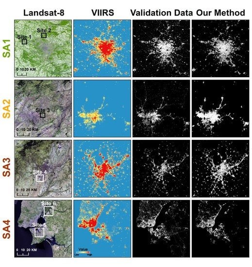
Next, we selected six sites in the four study areas to present detailed extraction results (Figure 6). Although the results derived by our method and FROM-GLC were both accurate, our method outperformed FROM-GLC in eliminating interference from bare land (Sites 1 and 2). In contrast, our method experienced limitations in road extraction, and the results were slightly poorer than those of FROM-GLC (Site 6). GUL provided good delineation of built-up areas in Sites 5 and 6; however, it overestimated built-up areas in Sites 1 and 2 (where built-up areas were mixed with bare land), showing similarity to the FROM-GLC results. In addition, GUL did not capture the built-up areas in sites 3 and 4. The use of the PII and VIIRS nighttime lights data to extract built-up areas in these six sites thus produced unsatisfying results. The PII extracted excessive built-up areas in Sites 1–4 and failed to identify the built-up areas in Sites 5 and 6. Meanwhile, the built-up areas extracted by using only VIIRS nighttime lights data greatly exceeded the actual built-up area in all six sites.
Lastly, we compared the areas extracted by our method with the areas in the reference data to further verify the accuracy of the built-up area extraction (Figure 7). We divided the four study areas using 3 × 3 km grids and calculated the built-up areas in each grid; the maximum size of the built-up areas in each grid was 9 km2. If the fit line was closer to the 1:1 line or had a stronger R2 correlation, it indicated that the extracted built-up areas were more accurate. The results showed that the R2 correlations in all four study areas were greater than 0.9 when using our method. The slope of Study Area 2 (Ankara) and 3 (Madrid) slightly deviated from the 1:1 line. This is consistent with the accuracy assessment in Figure 5, in which accuracy levels for these two study areas were slightly lower than those for Study Areas 1 (Paris) and 4 (Lisbon). In addition, we found that the slope of the line of best fit for most built-up area products was lower than the 1:1 line (Figures S2–S5). This difference indicates that some existing built-up area products overestimated the actual built-up areas, which corroborates findings from previous studies [15,19].
4. Discussion
The use of training samples and adaptive thresholds ensures our method’s high efficiency. To verify the quality of the built-up area training samples that we chose, we randomly selected six built-up area training sample sites from each study area. A comparison with Google Earth high-resolution imagery shows that the built-up training samples of our method not only had a diverse distribution, which contained urban and rural areas, but also accurately removed interference from other land cover types, particularly rivers and green spaces like parks in urban areas (Figure 8). Obtaining quality built-up training samples also depends on adaptive thresholding. Helpful in this regard, the Otsu algorithm, which we employ, can automatically segment and obtain accurate water and vegetation masks. The optimal thresholds were mostly located at the bottom of the two peaks in the histograms (Figure 9), which ensured the accuracy of the built-up training samples.
The selection of built-up target areas affects the built-up area extraction results. If the target areas are too large or too small, built-up areas may be overestimated or underestimated. Considering that VIIRS nighttime lights data values vary according to the intensity of human activities in different regions, the results obtained with only a single threshold may miss built-up areas in certain regions. This makes it potentially difficult to accurately derive built-up areas across all regions. To resolve this issue, our method segmented the VIIRS nighttime lights data using the Jenks natural breaks algorithm and acquired automated adaptive built-up target areas. Comparing the results with the Google Earth imagery confirmed that despite the omission of some road networks, the built-up target areas still represented the approximate spatial distribution of built-up areas across the four different cities and eliminated interference of bare land (Figure 10). This cross-comparison demonstrates that our method can successfully obtain fine built-up area results.
5. Conclusions
In this study, we combined VIIRS nighttime lights data and Landsat-8 multispectral imagery and developed a new method for built-up area extraction. Using adaptive thresholding, we acquired high-quality training samples automatically based on the VIIRS data and water and vegetation masks generated by Landsat-8 imagery. Next, we used the training samples to classify Landsat-8 imagery in order to obtain preliminary results for built-up areas. Lastly, we automatically derived and then superimposed built-up target areas onto the built-up area preliminary results, leading to the refinement of our built-up area classification results. Ultimately, our method significantly improved the extraction efficiency of built-up area. Our method had an overall accuracy exceeding 94.7% compared to the HRL IMD 2015 reference data. This represents a significant improvement over the FROM-GLC and GUL built-up area products, which required extensive and time-consuming manual post-processing.
Our approach still contains some limitations. For example, both VIIRS nighttime lights and Landat-8 imagery are limited by cloudiness, which is a challenge when applying our method globally, especially in tropic areas. However, considering that built-up areas do not change very rapidly, we can find some suitable cloudless nighttime lights and Landsat-8 data within 1 year to identify built-up areas. Additionally, the built-up target areas used in this study omitted certain road networks, resulting in an underestimation of built-up areas. This issue relates to the relatively low spatial resolution of VIIRS nighttime data, in which road networks appear as simply 1 pixel. In future efforts to improve built-up area extraction methods, it may be useful to consider using nighttime lights data with higher spatial resolution. One possibility is the 130-m resolution imagery from Luojia-1, a CubeSat-sized Earth observing satellite launched by China in mid-2018, which can detect lights across a higher dynamic range and with finer spatial details than VIIRS [65].
By experimenting with the built-up area extraction results in four study areas, our method takes full advantage of VIIRS nighttime lights and Landsat-8 multispectral imagery to efficiently extract built-up areas with high accuracy. The results eliminated the interference from non-built-up areas, particularly bare land. Our method’s major advantage is that it automatically selects training samples and determines adaptive thresholds according to the distribution of built-up areas in different regions. Compared to existing methods, this approach greatly improves the efficiency and accuracy of built-up area extraction. This methodological advance promises significant benefits for further global thematic mapping and dynamic change monitoring of built-up areas. Innovations such as these, which allow refined analysis of the spatial and temporal dynamics of the expansion of the built environment and its consequences for nature and society, are critical as the planet continues to urbanize and develop.
Supplementary Materials
The following are available online at https://www.mdpi.com/2072-4292/11/13/1571/s1, Figure S1: VIIRS nighttime lights categorized using the Jenks natural breaks algorithm in an example area (Study Area 1, Paris). Figures S2–S5: Built-up area scatter plots. The scatterplots compare the percentages of built-up areas using validation data in 9 km2 grids against those of (a) our method, (b) FROM-GLC, (c) GUL, (d) PII in Study Area 1 (Paris), Study Area 2 (Ankara), Study Area 3 (Madrid), Study Area 4 (Lisbon), respectively. Table S1: Percentages of pixels with DN = 0 and DN > high threshold in the four study areas.
Author Contributions
C.L., K.Y., and M.L. designed the study. C.L. performed the data analysis. C.L. and K.Y. wrote the paper with contributions from all authors.
Funding
This research was funded by the National Key R&D Program of China (No. 2017YFB0504205), the National Natural Science Foundation of China (No. 41871327), and the Fundamental Research Funds for the Central Universities (No. 14380070).
Acknowledgments
We are grateful to anonymous reviewers and members of the editorial team for advice.
Conflicts of Interest
The authors declare no conflict of interest.
References
- Schneider, A.; Friedl, M.A.; Potere, D. Mapping global urban areas using MODIS 500-m data: New methods and datasets based on ‘urban ecoregions’. Remote Sens. Environ. 2010, 114, 1733–1746. [Google Scholar] [CrossRef]
- Lu, D.; Weng, Q. Use of impervious surface in urban land-use classification. Remote Sens. Environ. 2006, 102, 146–160. [Google Scholar] [CrossRef]
- Weng, Q. Remote sensing of impervious surfaces in the urban areas: Requirements, methods, and trends. Remote Sens. Environ. 2012, 117, 34–49. [Google Scholar] [CrossRef]
- Foley, J.A.; DeFries, R.; Asner, G.P.; Barford, C.; Bonan, G.; Carpenter, S.R.; Chapin, F.S.; Coe, M.T.; Daily, G.C.; Gibbs, H.K.; et al. Global Consequences of Land Use. Science 2005, 309, 570–574. [Google Scholar] [CrossRef] [PubMed] [Green Version]
- Grimm, N.B.; Faeth, S.H.; Golubiewski, N.E.; Redman, C.L.; Wu, J.; Bai, X.; Briggs, J.M. Global Change and the Ecology of Cities. Science 2008, 319, 756–760. [Google Scholar] [CrossRef] [Green Version]
- He, C.; Liu, Z.; Tian, J.; Ma, Q. Urban expansion dynamics and natural habitat loss in China: A multiscale landscape perspective. Glob. Chang. Biol. 2014, 20, 2886–2902. [Google Scholar] [CrossRef]
- McDonald, R.I.; Kareiva, P.; Forman, R.T.T. The implications of current and future urbanization for global protected areas and biodiversity conservation. Biol. Cons. 2008, 141, 1695–1703. [Google Scholar] [CrossRef]
- Tran, D.X.; Pla, F.; Latorre-Carmona, P.; Myint, S.W.; Caetano, M.; Kieu, H.V. Characterizing the relationship between land use land cover change and land surface temperature. ISPRS J. Photogramm. Remote Sens. 2017, 124, 119–132. [Google Scholar] [CrossRef] [Green Version]
- Sofia, G.; Roder, G.; Dalla Fontana, G.; Tarolli, P. Flood dynamics in urbanised landscapes: 100 years of climate and humans’ interaction. Sci. Rep. 2017, 7, 40527. [Google Scholar] [CrossRef]
- IPCC. Climate Change, Adaptation, and Vulnerability. Organ. Environ. 2014, 24, 535–613. [Google Scholar]
- Zhang, G.; Yao, T.; Chen, W.; Zheng, G.; Shum, C.K.; Yang, K.; Piao, S.; Sheng, Y.; Yi, S.; Li, J.; et al. Regional differences of lake evolution across China during 1960s–2015 and its natural and anthropogenic causes. Remote Sens. Environ. 2019, 221, 386–404. [Google Scholar] [CrossRef]
- Ougaard, M. The Transnational State and the Infrastructure Push. New Political Econ. 2018, 23, 128–144. [Google Scholar] [CrossRef]
- Esch, T.; Heldens, W.; Hirner, A.; Keil, M.; Marconcini, M.; Roth, A.; Zeidler, J.; Dech, S.; Strano, E. Breaking new ground in mapping human settlements from space—The Global Urban Footprint. ISPRS J. Photogramm. Remote Sens. 2017, 134, 30–42. [Google Scholar] [CrossRef]
- Potere, D.; Schneider, A.; Angel, S.; Civco, D.L. Mapping urban areas on a global scale: Which of the eight maps now available is more accurate? Int. J. Remote Sens. 2009, 30, 6531–6558. [Google Scholar] [CrossRef]
- Liu, X.; Hu, G.; Chen, Y.; Li, X.; Xu, X.; Li, S.; Pei, F.; Wang, S. High-resolution multi-temporal mapping of global urban land using Landsat images based on the Google Earth Engine Platform. Remote Sens. Environ. 2018, 209, 227–239. [Google Scholar] [CrossRef]
- Gong, P.; Wang, J.; Yu, L.; Zhao, Y.; Zhao, Y.; Liang, L.; Niu, Z.; Huang, X.; Fu, H.; Liu, S.; et al. Finer resolution observation and monitoring of global land cover: First mapping results with Landsat TM and ETM+ data. Int. J. Remote Sens. 2012, 34, 2607–2654. [Google Scholar] [CrossRef]
- Chen, J.; Chen, J.; Liao, A.; Cao, X.; Chen, L.; Chen, X.; He, C.; Han, G.; Peng, S.; Lu, M.; et al. Global land cover mapping at 30m resolution: A POK-based operational approach. ISPRS J. Photogramm. Remote Sens. 2015, 103, 7–27. [Google Scholar] [CrossRef] [Green Version]
- Dell’Acqua, F.; Gamba, P. Discriminating urban environments using multiscale texture and multiple SAR images. Int. J. Remote Sens. 2006, 27, 3797–3812. [Google Scholar] [CrossRef]
- Ban, Y.; Jacob, A.; Gamba, P. Spaceborne SAR data for global urban mapping at 30 m resolution using a robust urban extractor. ISPRS J. Photogramm. Remote Sens. 2015, 103, 28–37. [Google Scholar] [CrossRef]
- Zhou, S.; Deng, Y.; Wang, R.; Li, N.; Si, Q. Effective Mapping of Urban Areas Using ENVISAT ASAR, Sentinel-1A, and HJ-1-C Data. IEEE Geosci. Remote Sens. Lett. 2017, 14, 891–895. [Google Scholar] [CrossRef]
- He, C.; Shi, P.; Xie, D.; Zhao, Y. Improving the normalized difference built-up index to map urban built-up areas using a semiautomatic segmentation approach. Remote Sens. Lett. 2010, 1, 213–221. [Google Scholar] [CrossRef] [Green Version]
- Sabo, F.; Corbane, C.; Florczyk, A.J.; Ferri, S.; Pesaresi, M.; Kemper, T. Comparison of built-up area maps produced within the global human settlement framework. Trans. GIS 2018, 22, 1406–1436. [Google Scholar] [CrossRef]
- Goldblatt, R.; Stuhlmacher, M.F.; Tellman, B.; Clinton, N.; Hanson, G.; Georgescu, M.; Wang, C.; Serrano-Candela, F.; Khandelwal, A.K.; Cheng, W.-H.; et al. Using Landsat and nighttime lights for supervised pixel-based image classification of urban land cover. Remote Sens. Environ. 2018, 205, 253–275. [Google Scholar] [CrossRef]
- Guo, W.; Zhang, Y.; Gao, L. Using VIIRS-DNB and landsat data for impervious surface area mapping in an arid/semiarid region. Remote Sens. Lett. 2018, 9, 587–596. [Google Scholar] [CrossRef]
- Wang, R.; Wan, B.; Guo, Q.; Hu, M.; Zhou, S. Mapping Regional Urban Extent Using NPP-VIIRS DNB and MODIS NDVI Data. Remote Sens. 2017, 9, 862. [Google Scholar] [CrossRef]
- Zhang, Q.; Wang, P.; Chen, H.; Huang, Q.; Jiang, H.; Zhang, Z.; Zhang, Y.; Luo, X.; Sun, S. A novel method for urban area extraction from VIIRS DNB and MODIS NDVI data: A case study of Chinese cities. Int. J. Remote Sens. 2017, 38, 6094–6109. [Google Scholar] [CrossRef]
- Rasul, A.; Balzter, H.; Ibrahim, R.G.; Hameed, M.H.; Wheeler, J.; Adamu, B.; Ibrahim, S.; Najmaddin, M.P. Applying Built-Up and Bare-Soil Indices from Landsat 8 to Cities in Dry Climates. Land 2018, 7, 81. [Google Scholar] [CrossRef]
- Li, K.; Chen, Y. A Genetic Algorithm-Based Urban Cluster Automatic Threshold Method by Combining VIIRS DNB, NDVI, and NDBI to Monitor Urbanization. Remote Sens. 2018, 10, 277. [Google Scholar] [CrossRef]
- Li, X.; Zhou, Y. Urban mapping using DMSP/OLS stable night-time light: A review. Int. J. Remote Sens. 2017, 38, 6030–6046. [Google Scholar] [CrossRef]
- Shi, K.; Huang, C.; Yu, B.; Yin, B.; Huang, Y.; Wu, J. Evaluation of NPP-VIIRS night-time light composite data for extracting built-up urban areas. Remote Sens. Lett. 2014, 5, 358–366. [Google Scholar] [CrossRef]
- Cao, X.; Chen, J.; Imura, H.; Higashi, O. A SVM-based method to extract urban areas from DMSP-OLS and SPOT VGT data. Remote Sens. Environ. 2009, 113, 2205–2209. [Google Scholar] [CrossRef]
- Xie, Y.; Weng, Q. Spatiotemporally enhancing time-series DMSP/OLS nighttime light imagery for assessing large-scale urban dynamics. ISPRS J. Photogramm. Remote Sens. 2017, 128, 1–15. [Google Scholar] [CrossRef]
- Guo, W.; Lu, D.; Wu, Y.; Zhang, J. Mapping Impervious Surface Distribution with Integration of SNNP VIIRS-DNB and MODIS NDVI Data. Remote Sens. 2015, 7, 12459–12477. [Google Scholar] [CrossRef] [Green Version]
- Latifovic, R.; Pouliot, D.; Olthof, I. Circa 2010 Land Cover of Canada: Local Optimization Methodology and Product Development. Remote Sens. 2017, 9, 1098. [Google Scholar] [CrossRef]
- Huang, X.; Hu, T.; Li, J.; Wang, Q.; Benediktsson, J.A. Mapping Urban Areas in China Using Multisource Data With a Novel Ensemble SVM Method. IEEE Trans. Geosci. Remote Sens. 2018, 56, 4258–4273. [Google Scholar] [CrossRef]
- Zhou, Y.; Smith, S.J.; Elvidge, C.D.; Zhao, K.; Thomson, A.; Imhoff, M. A cluster-based method to map urban area from DMSP/OLS nightlights. Remote Sens. Environ. 2014, 147, 173–185. [Google Scholar] [CrossRef]
- Pesaresi, M.; Ehrlich, D.; Ferri, S.; Florczyk, A.; Manuel, C.F.S.; Halkia, S.; Maria, J.A.; Thomas, K.; Pierre, S.; Vasileios, S. Operating Procedure for the Production of the Global Human Settlement Layer from Landsat Data of the Epochs 1975, 1990, 20001975, 1990, 2000, and 2014; Publications Office of the European Union: Luxembourg, 2016. [Google Scholar]
- Corbane, C.; Pesaresi, M.; Politis, P.; Syrris, V.; Florczyk, A.J.; Soille, P.; Maffenini, L.; Burger, A.; Vasilev, V.; Rodriguez, D.; et al. Big earth data analytics on Sentinel 1 and Landsat imagery in support to global human settlements mapping. Big Earth Data 2017, 1, 118–144. [Google Scholar] [CrossRef]
- Wang, P.; Huang, C.; Brown de Colstoun, E.C.; Tilton, J.C.; Tan, B. Global Human Built-Up And Settlement Extent (HBASE) Dataset From Landsat; NASA Socioeconomic Data and Applications Center (SEDAC): Palisades, NY, USA, 2017. [Google Scholar]
- The National Land Cover Database. Available online: https://www.usgs.gov/centers/eros/science/national-land-cover-database (accessed on 15 December 2018).
- Copernicus Land Monitoring Service—High Resolution Layer Imperviousness: Product Specifications Document. Available online: https://land.copernicus.eu/user-corner/technical-library/hrl-imperviousness-technical-document-prod-2015 (accessed on 20 April 2019).
- Florczyk, A.J.; Ferri, S.; Syrris, V.; Kemper, T.; Halkia, M.; Soille, P.; Pesaresi, M. A New European Settlement Map From Optical Remotely Sensed Data. IEEE J. Sel. Top. Appl. Earth Observ. Remote Sens. 2016, 9, 1978–1992. [Google Scholar] [CrossRef]
- Loveland, T.R.; Irons, J.R. Landsat 8: The plans, the reality, and the legacy. Remote Sens. Environ. 2016, 185, 1–6. [Google Scholar] [CrossRef] [Green Version]
- Vermote, E.; Justice, C.; Claverie, M.; Franch, B. Preliminary analysis of the performance of the Landsat 8/OLI land surface reflectance product. Remote Sens. Environ. 2016, 185, 46–56. [Google Scholar] [CrossRef]
- Roy, D.P.; Wulder, M.A.; Loveland, T.R.; Woodcock, C.E.; Allen, R.G.; Anderson, M.C.; Helder, D.; Irons, J.R.; Johnson, D.M.; Kennedy, R.; et al. Landsat-8: Science and product vision for terrestrial global change research. Remote Sens. Environ. 2014, 145, 154–172. [Google Scholar] [CrossRef] [Green Version]
- Bennett, M.M.; Smith, L.C. Advances in using multitemporal night-time lights satellite imagery to detect, estimate, and monitor socioeconomic dynamics. Remote Sens. Environ. 2017, 192, 176–197. [Google Scholar] [CrossRef]
- Elvidge, C.D.; Baugh, K.E.; Zhizhin, M.; Hsu, F.-C. Why VIIRS data are superior to DMSP for mapping nighttime lights. Proc. Asia Pac. Adv. Netw. 2013, 35, 62–69. [Google Scholar] [CrossRef]
- Miller, S.; Straka, W.; Mills, S.; Elvidge, C.; Lee, T.; Solbrig, J.; Walther, A.; Heidinger, A.; Weiss, S. Illuminating the Capabilities of the Suomi National Polar-Orbiting Partnership (NPP) Visible Infrared Imaging Radiometer Suite (VIIRS) Day/Night Band. Remote Sens. 2013, 5, 6717–6766. [Google Scholar] [CrossRef] [Green Version]
- Elvidge, C.; Hsu, F.-C.; Baugh, K.; Ghosh, T. National Trends in Satellite-Observed Lighting: 1992–2012. In Global Urban Monitoring and Assessment through Earth Observation; CRC Press: London, UK, 2014; Volume 23, pp. 97–120. [Google Scholar]
- HRL Imperviousness Degree 2015 Validation Report. Available online: https://land.copernicus.eu/user-corner/technical-library/hrl-2015-imperviousness-validation-report (accessed on 10 May 2019).
- North, M.A. A Method for Implementing a Statistically Significant Number of Data Classes in the Jenks Algorithm. In Proceedings of the 2009 Sixth International Conference on Fuzzy Systems and Knowledge Discovery, Tianjin, China, 14–16 August 2009; pp. 35–38. [Google Scholar]
- Zhou, Y.; Tu, M.; Wang, S.; Liu, W. A Novel Approach for Identifying Urban Built-Up Area Boundaries Using High-Resolution Remote-Sensing Data Based on the Scale Effect. ISPRS Int. J. Geo. Inf. 2018, 7, 135. [Google Scholar] [CrossRef]
- Jenks, G.F. The Data Model Concept in Statistical Mapping. Int. Yearb. Cartogr. 1967, 7, 186–190. [Google Scholar]
- Xu, H. Modification of normalised difference water index (NDWI) to enhance open water features in remotely sensed imagery. Int. J. Remote Sens. 2007, 27, 3025–3033. [Google Scholar] [CrossRef]
- Myneni, R.B.; Hall, F.G.; Sellers, P.J.; Marshak, A.L. The interpretation of spectral vegetation indexes. IEEE Trans. Geosci. Remote Sens 1995, 33, 481–486. [Google Scholar] [CrossRef]
- Otsu, N. A threshold selection method from gray-level histograms. IEEE Trans. Syst. Man Cybern. Syst. 1979, 9, 62–66. [Google Scholar] [CrossRef]
- Huang, C.; Song, K.; Kim, S.; Townshend, J.R.G.; Davis, P.; Masek, J.G.; Goward, S.N. Use of a dark object concept and support vector machines to automate forest cover change analysis. Remote Sens. Environ. 2008, 112, 970–985. [Google Scholar] [CrossRef]
- Huang, C.; Davis, L.S.; Townshend, J.R.G. An assessment of support vector machines for land cover classification. Int. J. Remote Sens. 2002, 23, 725–749. [Google Scholar] [CrossRef]
- Li, C.; Wang, J.; Wang, L.; Hu, L.; Gong, P. Comparison of Classification Algorithms and Training Sample Sizes in Urban Land Classification with Landsat Thematic Mapper Imagery. Remote Sens. 2014, 6, 964–983. [Google Scholar] [CrossRef] [Green Version]
- Herold, M.; Gardner, M.E.; Roberts, D.A. Spectral resolution requirements for mapping urban areas. IEEE Trans. Geosci. Remote Sens. 2003, 41, 1907–1919. [Google Scholar] [CrossRef] [Green Version]
- Okujeni, A.; van der Linden, S.; Hostert, P. Extending the vegetation–impervious–soil model using simulated EnMAP data and machine learning. Remote Sens. Environ. 2015, 158, 69–80. [Google Scholar] [CrossRef]
- Popular Repositories. Available online: https://github.com/njuRS (accessed on 9 March 2019).
- Tian, Y.; Xu, Y.; Yang, X. Perpendicular Impervious Index for Remote Sensing of Multiple Impervious Surface Extraction in Cities. Acta Geod. Cartogr. Sin. 2017, 46, 468–477. [Google Scholar] [CrossRef]
- Liu, C.; Yang, K.; Cheng, L.; Li, M.; Guo, Z. A comparison of Landsat8 impervious surface extraction methods. Remote Sens. Land Resour. (accepted).
- Jiang, W.; He, G.; Long, T.; Guo, H.; Yin, R.; Leng, W.; Liu, H.; Wang, G. Potentiality of Using Luojia 1-01 Nighttime Light Imagery to Investigate Artificial Light Pollution. Sensors 2018, 18, 2900. [Google Scholar] [CrossRef]
Figure 1.
Location of the study areas. The Landsat-8 remotely-sensed images (in which Band 7 = Red, Band 6 = Green, and Band 4 = Blue (R7G6B4)) of the four study areas are shown.
Figure 1.
Location of the study areas. The Landsat-8 remotely-sensed images (in which Band 7 = Red, Band 6 = Green, and Band 4 = Blue (R7G6B4)) of the four study areas are shown.

Figure 2.
Flowchart of our built-up area extraction method.

Figure 3.
Results of the extraction of built-up areas according to different methods. For the reference data and our method, white pixels correspond to the built-up area while black pixels represent non-built-up areas.
Figure 3.
Results of the extraction of built-up areas according to different methods. For the reference data and our method, white pixels correspond to the built-up area while black pixels represent non-built-up areas.

Figure 4.
Comparison of results of the extraction of built-up areas according to different methods. The first column shows the Landsat-8 remote-sensing images (RG6B4); the second column shows the HRL IMD2015 reference data; the third column shows the built-up area extraction results using our method, and the fourth through seventh columns show the built-up area results for FROM-GLC, GUL, PII, and VIIRS.

Figure 5.
Comparison of built-up area accuracy and associated measures for FROM-GLC, PII, GUL, and VIIRS. (a) Overall accuracy; (b) Kappa coefficient; (c) Producer’s accuracy; (d) User’s accuracy.
Figure 5.
Comparison of built-up area accuracy and associated measures for FROM-GLC, PII, GUL, and VIIRS. (a) Overall accuracy; (b) Kappa coefficient; (c) Producer’s accuracy; (d) User’s accuracy.

Figure 6.
Comparison of built-up area extraction results across local sites using our method, FROM-GLC, GUL, PII, and VIIRS. These results are compared with the Landsat-8 and HRL IMD 2015 data. The locations of the six sites are shown in Figure 3.
Figure 6.
Comparison of built-up area extraction results across local sites using our method, FROM-GLC, GUL, PII, and VIIRS. These results are compared with the Landsat-8 and HRL IMD 2015 data. The locations of the six sites are shown in Figure 3.

Figure 7.
Built-up area scatterplots. The scatterplots compare the percentages of built-up areas in four study areas: (a) SA1 (Paris); (b) SA2 (Ankara); (c) SA3 (Madrid); and (d) SA4 (Lisbon) found by our method with the reference data in 9 km2 grids.
Figure 7.
Built-up area scatterplots. The scatterplots compare the percentages of built-up areas in four study areas: (a) SA1 (Paris); (b) SA2 (Ankara); (c) SA3 (Madrid); and (d) SA4 (Lisbon) found by our method with the reference data in 9 km2 grids.

Figure 8.
Distribution map of built-up area sample sites. The yellow polygonal areas represent the built-up area sample sites automatically selected by our method. Six built-up area sample sites (white polygon areas) were selected in the four study areas. Figure 8A–F show the results of superimposing built-up area sample sites onto Google Earth high-resolution remote-sensing imagery.

Figure 9.
Histograms of frequency distributions of vegetation and water body indices in the four study areas. The red lines indicate the optimal threshold position of the vegetation and water masks automatically acquired by the Otsu method.
Figure 9.
Histograms of frequency distributions of vegetation and water body indices in the four study areas. The red lines indicate the optimal threshold position of the vegetation and water masks automatically acquired by the Otsu method.

Figure 10.
Distribution maps of built-up target areas. The white polygonal areas represent the built-up target area selected using the VIIRS nighttime lights data.
Figure 10.
Distribution maps of built-up target areas. The white polygonal areas represent the built-up target area selected using the VIIRS nighttime lights data.


Table 1.
Global and regional high-resolution built-up area products.
| Abbreviation | Map | Producer | Reference Year(s) | Resolution | Extent | Data | Method | Accuracy | Reference |
|---|---|---|---|---|---|---|---|---|---|
| GLC30 | GlobeLand30 | NGCC | 2010 | 30 m | Global | Landsat | Supervised classification based on POK | UA: 86.7% | [17] |
| FROM-GLC | Finer Resolution Observation and Monitoring of Global Land Cover | THU | 2010, 2015, 2017 | 30 m | Global | Landsat | Supervised classification | UA: 30.8% (2010) | [16] |
| GUL | Global Urban Land | SYSU | 1990–2015, every five years | 30 m | Global | Landsat, DMSP-OLS | NUACI | TA: 81%-84% | [15] |
| GHS | Global Human Settlement | JRC | 1975, 1990, 2000, 2014 | 38 m | Global | Landsat | Supervised classification based on SML | TA: 89% | [37] |
| 2016 | 20 m | Global | Sentinel-1 | Supervised classification based on SML | ** | [38] | |||
| HBASE | Global Human Built-up And Settlement Extent | NASA | 2010 | 30 m | Global | Landsat | Supervised classification based on texture features | ** | [39] |
| GUF | Global Urban Footprint | DLR | 2011 | 12 m | Global | TerraSAR X, TanDEM X | Unsupervised classification based on texture features | TA: 85% | [13] |
| NLCD | National Land Cover Database | MRLC | 2001, 2006, 2011 | 30 m | USA | Landsat | Supervised classification based on decision-tree classification | RMSE: 6.86-13.12% (2006) | [40] |
| HRL IMD | High Resolution Layer Imperviousness Degree | EEA | 2006, 2009, 2012, 2015 | 20 m | Europe | Landsat, SPOT-5 | Supervised classification | UA>90% PA>90% | [41] |
| ESM | European Settlement Map | JRC | 2012 | 2.5 m, 10 m | Europe | SPOT-5, SPOT-6 | Supervised classification based on SML | TA>95% | [42] |
Abbreviations: NGCC, National Geomatics Center of China; THU, Tsinghua University; SYSU, Sun Yat-sen University; JRC, Joint Research Centre; NASA, National Aeronautics and Space Administration; DLR, German Aerospace Center; MRLC, Multi-Resolution Land Characteristics Consortium; EEA, European Environment Agency; POK, pixel-object-knowledge; SML, Symbolic Machine Learning; OA, overall accuracy; UA, user’s accuracy; RMSE, root-mean-square error; PA, producer’s accuracy; ** means not mentioned in the product metadata. The template details the sections that can be used in a manuscript. Note that each section has a corresponding style, which can be found in the ‘Styles’ menu of Word. Sections that are not mandatory are listed as such. The section titles given are for Articles. Review papers and other article types have a more flexible structure.
Table 2.
Landsat-8 images for the four study areas.
| Study Area | Path-Row | Imaging Date |
|---|---|---|
| 1 (Paris) | 199-26 | 2015-09-27 |
| 2 (Ankara) | 177-32 | 2015-11-04 |
| 3 (Madrid) | 201-32 | 2015-09-25 |
| 4 (Lisbon) | 204-33 | 2015-06-26 |
© 2019 by the authors. Licensee MDPI, Basel, Switzerland. This article is an open access article distributed under the terms and conditions of the Creative Commons Attribution (CC BY) license (http://creativecommons.org/licenses/by/4.0/).
Share and Cite
MDPI and ACS Style
Liu, C.; Yang, K.; Bennett, M.M.; Guo, Z.; Cheng, L.; Li, M. Automated Extraction of Built-Up Areas by Fusing VIIRS Nighttime Lights and Landsat-8 Data. Remote Sens. 2019, 11, 1571. https://doi.org/10.3390/rs11131571
AMA Style
Liu C, Yang K, Bennett MM, Guo Z, Cheng L, Li M. Automated Extraction of Built-Up Areas by Fusing VIIRS Nighttime Lights and Landsat-8 Data. Remote Sensing. 2019; 11(13):1571. https://doi.org/10.3390/rs11131571
Chicago/Turabian StyleLiu, Chang, Kang Yang, Mia M. Bennett, Ziyan Guo, Liang Cheng, and Manchun Li. 2019. "Automated Extraction of Built-Up Areas by Fusing VIIRS Nighttime Lights and Landsat-8 Data" Remote Sensing 11, no. 13: 1571. https://doi.org/10.3390/rs11131571
Note that from the first issue of 2016, this journal uses article numbers instead of page numbers. See further details here.