Asymmetric Effects of Daytime and Nighttime Warming on Boreal Forest Spring Phenology
by
 , ,
, ,
Guorong Deng
1 ,
,
Hongyan Zhang
1,*,
Xiaoyi Guo
1,
Yu Shan
1,2,
Hong Ying
1,
Wu Rihan
1,
Hui Li
1 and 
Yangli Han
3 1
School of Geographical Sciences, Northeast Normal University, Changchun 130024, China
2
Inner Mongolia Key Laboratory of Remote Sensing and Geographic Information System, Hohhot 010022, China
3
School of Geographical Sciences, Nanjing Normal University, Nanjing 210023, China
*
Author to whom correspondence should be addressed.
Remote Sens. 2019, 11(14), 1651; https://doi.org/10.3390/rs11141651
Submission received: 4 June 2019
/
Revised: 9 July 2019
/
Accepted: 9 July 2019
/
Published: 11 July 2019
(This article belongs to the Special Issue Monitoring Vegetation Phenology: Trends and Anomalies)
Abstract
:Vegetation phenology is the most intuitive and sensitive biological indicator of environmental conditions, and the start of the season (SOS) can reflect the rapid response of terrestrial ecosystems to climate change. At present, the model based on mean temperature neglects the role of the daytime maximum temperature (TMAX) and the nighttime minimum temperature (TMIN) in providing temperature accumulation and cold conditions at leaf onset. This study analyzed the spatiotemporal variations of spring phenology for the boreal forest from 2001 to 2017 based on the moderate-resolution imaging spectro-radiometer (MODIS) enhanced vegetation index (EVI) data (MOD13A2) and investigated the asymmetric effects of daytime and nighttime warming on the boreal forest spring phenology during TMAX and TMIN preseason by partial correlation analysis. The results showed that the spring phenology was delayed with increasing latitude of the boreal forest. Approximately 91.37% of the region showed an advancing trend during the study period, with an average advancement rate of 3.38 ± 0.08 days/decade, and the change rates of different land cover types differed, especially in open shrubland. The length of the TMIN preseason was longer than that of the TMAX preseason and diurnal temperatures showed an asymmetrical increase during different preseasons. The daytime and nighttime warming effects on the boreal forest are asymmetrical. The TMAX has a greater impact on the vegetation spring phenology than TMIN as a whole and the effect also has seasonal differences; the TMAX mainly affects the SOS in spring, while TMIN has a greater impact in winter. The asymmetric effects of daytime and nighttime warming on the SOS in the boreal forest were highlighted in this study, and the results suggest that diurnal temperatures should be added to the forest terrestrial ecosystem model.
1. Introduction
Vegetation and climate change have a complex interaction, as climate change affects vegetation growth, and vegetation change has a specific feedback effect on the regional climate [1,2]. Spring phenology is an important factor in measuring dynamic vegetation landscape changes, and has been widely studied in different research fields [3,4,5]. The start of the season (SOS), as an important spring phenology indicator, is very sensitive to global climate change. However, the traditional dynamic phenological monitoring is mainly based on ground observations, which are difficult to obtain on a larger spatial scale because of the high costs and low efficiency [6,7]. The development of remote sensing technology provided a new method for the determination of vegetation phenological parameters [8,9,10,11,12]. These studies based on long time series satellite data have dynamically monitored vegetation phenology at different scales, such as hemisphere [13,14], continental [6,15,16] and national [17] scales, and the SOS showed an apparent advancing trend during the past three decades in the Northern Hemisphere [16,18,19]. Changes in spring phenology also alter ecosystem functions, leading to changes in carbon, water, and energy balances [20,21,22]. Therefore, researching the SOS response to current climate change is helpful in understanding future vegetation responses to climate change and the dynamic changes in ecosystems.
The onset of vegetation green-up is not an instantaneous process. It requires an adequate accumulation of heat during preseason dormancy and has a specific demand for chilling conditions [23]. Previous vegetation phenology studies that were based on mean temperature neglected the role of daytime and nighttime temperatures in providing temperature accumulation and cold conditions. In fact, there is a trend in most parts of the world where nighttime warming is faster than daytime warming [24,25], resulting in a narrower diurnal temperature range (DTR). Because most of the vegetation photosynthesis that occurs during the daytime is influenced by the maximum temperature during the daytime (TMAX), and respiration occurs throughout the entire day and is affected by both TMAX and minimum temperature during the nighttime (TMIN) [26], this diurnal warming pattern will have an asymmetric effect on plant growth and carbon absorption and consumption, which also have complex effects on phenology [27,28]. Based on the vegetation phenology mechanism, it is also indicated that the period in which daytime and nighttime temperatures actually affect vegetation phenology should be the preseason dormancy period of vegetation [29]. Thus, the length of the preseason period is particularly important for understanding the effects of daytime and nighttime temperatures on phenology.
Recent studies have shown that the increase in TMAX has a greater impact on the spring phenology than TMIN in the Northern Hemisphere [23]. However, the opposite conclusions have been obtained in particular areas, such as the Tibetan Plateau [30]. This difference may be due to the cold and dryness in the Tibetan Plateau. The increase in TMIN reduces the possibility of frost occurrence, while the increase in TMAX leads to the intensification of drought [31]. The seasonal SOS response to diurnal temperature has also attracted research focus [32]. For example, in the temperate grasslands of China, Shen et al. found that SOS is affected most strongly by winter TMAX and by spring TMIN [33]. However, most of these studies are based on hemispheric scale and grasslands, and the impact mechanism of daytime and nighttime temperature on forests at the regional scale remains to be further studied.
The boreal forest is located in the mid-high latitudes of the Northern Hemisphere and is one of the most sensitive and early responding forest regions to climate change in the world [34,35]. Temperature, precipitation, and solar radiation are the main driving factors that affect vegetation growth [36,37]. Although snow may delay the SOS, there is little evidence that precipitation has a significant impact on phenology in the boreal forest [21], and previous studies have also shown that the vegetation phenology is insensitive to the increase in CO2 in this area [29]. Thus, the boreal forest is an excellent place to explore the response of forest vegetation phenology to temperature changes, especially daytime and nighttime temperatures. The main objectives of this study are to (i) analyze the spatial and temporal patterns in the spring phenology of the boreal forest at the pixel scale; (ii) explore the spring phenological trends in different land cover types; (iii) reveal the lengths of the TMAX preseason and TMIN preseason and consider the changes in daytime and nighttime temperatures during the two preseasons; and (iv) clarify the asymmetric effects of daytime and nighttime temperatures on phenology during the study period. The flowchart of our study is shown in Figure 1.
2. Materials and Methods
2.1. Study Area
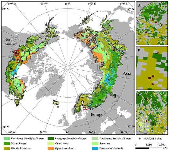
The boreal forest is a circular forest belt located in the middle and high latitudes of the Northern Hemisphere with latitudes ranging from 45°30′N to 71°18′N (Figure 2). The boundaries of the study area were published in 2009 by The Nature Conservancy (TNC) based on the Terrestrial Ecoregions of the World (TEOW) dataset [38]. The region is mainly affected by a temperate continental climate and is characterized by humid summers and dry, cold winters. The mean annual temperature is from −21.19 °C to 7.27 °C and decreases with increasing latitude. The average annual precipitation is from 80 mm to 2084 mm, and the precipitation distribution is quite different because the area is across different climate zones. Vegetation in the study area can be classified into eight generalized types: Mixed forest, deciduous broadleaf forest, deciduous needleleaf forest, and evergreen needleleaf forest, which are distributed along the southern boundary of the boreal forest. The grasslands, savannas, and woody savannas are concentrated in part of North America and Siberia and collectively constitute 59.45% of the area. Open shrubland is mainly distributed within the Arctic Circle.
The entire study area includes the following 18 main ecological regions classified by TEOW [38]: (a) Boreal Cordillera; (b) Boreal Shield; (c) East Siberian Taiga; (d) Eastern Canadian Forests; (e) Iceland Boreal Birch Forests and Alpine Tundra; (f) Interior Alaska-Yukon Lowland Taiga; (g) Kamchatka-Kurile Meadows and Space Forests; (h) Mid-Continental Canadian Forests; (i) Northeast Siberian Taiga; (j) Northern Canadian Shied Taiga; (k) Okhotsk-Manchurian Taiga; (l) Sakhalin Island Taiga; (m) Scandinavian and Russian Taiga; (n) Southern Hudson Bay Taiga; (o) Trans-Baikal Conifer Forests; (p) Taiga Plains; (q) Ural Montane Forests and Tundra; and (r) West Siberian Taiga.
2.2. Datasets
2.2.1. Meteorological Data
Climatic Research Unit (CRU, https://crudata.uea.ac.uk/cru/data/hrg/) grid data based on monthly observations at meteorological stations across the world’s land areas were used in combination with existing climatology to obtain absolute monthly values [26,39]. In this study, we used the CRU climatic dataset for the 2001 to 2017 period (version TS4.01), including TMAX, TMIN, DTR, monthly precipitation and cloudiness (representing solar radiation), with a spatial resolution of 0.5° × 0.5° for analyzing the relationships between diurnal warming and vegetation phenology.
2.2.2. MODIS Enhanced Vegetation Index
The enhanced vegetation index (EVI), which introduced the blue reflectance band and soil adjustment parameters to correct for the residual aerosol and canopy background [40,41,42], is more suitable for used in densely vegetated areas like the boreal forest than the normalized differential vegetation index (NDVI). In this study, we use the moderate resolution imaging spectro-radiometer (MODIS) EVI dataset (MOD13A2, collection 6) from January 2001 to December 2017 to extract the SOS and the end of season (EOS) data across the study area. The MOD13A2 product was obtained from the National Aeronautics and Space Administration (NASA) website (https://search.earthdata.nasa.gov) with a 16-day temporal resolution and 1-km spatial resolution.
2.2.3. FLUXNET Dataset
Net ecosystem exchange (NEE) was used to evaluate and validate SOS data extracted by MODIS EVI in this study. The daily NEE data are obtained from the FLUXNET 2015 dataset (http://fluxnet.fluxdata.org/). FLUXNET is a global network of micrometeorological tower sites that measure the exchanges of carbon dioxide (CO2), water vapor, and energy between terrestrial ecosystems and the atmosphere, and the shared data are processed by uniform quality control, interpolation, and splitting [43]. In this study, we selected data from 20 sites across the study area to remove the years with significant outliers (value = −9999) and ultimately identified 86 NEE verification points.
2.2.4. Landcover Dataset
We used MCD12C1 (collection 6) to classify different boreal forest land cover types. The dataset defines 17 types of land cover based on the International Geosphere-Biosphere Programme (IGBP) global vegetation classification scheme. Non-vegetation (water bodies, permanent snow and ice, barren), manmade (croplands, urban and built-up lands, cropland/natural vegetation mosaics) and over-small (evergreen broadleaf forests, closed shrublands, permanent wetlands) land cover types were removed in the study area. Deciduous broadleaf forest, deciduous needleleaf forest, evergreen needleleaf forest, mixed forest, grassland, savannas, woody savannas, and open shrubland are used to analyze in this paper. We also extracted land cover types that have not changed since 2001 to reduce the impact of land cover changes on phenology for research.
2.3. Methods
2.3.1. Vegetation Phenology from MODIS EVI Data
The MOD13A2 product uses the maximum value composite (MVC) method to remove part of the noise, but the composite value is still subject to interference from uncorrected aerosol and oblique solar elevation angle, both of which decrease the EVI value and produce curves that are jagged and irregular [44]. Therefore, to extract SOS, it is necessary to denoise and smooth the EVI time series; that is, accomplish a time series reconstruction [45]. The double logistic function (DL), Savitzky–Golay filter (SG) and asymmetric Gaussian model (AG) are the three most widely used methods for time series fitting [7,46,47,48], and each method has advantages. DL is suitable for extracting phenological characteristics of different vegetation types without artificial thresholds and performs better in high latitudes with long-term snow and ice cover [8,47,49]. SG can retain the real details of the EVI time series and smooth the curve in accordance with the vegetation growth law, which is beneficial to high precision information extraction of vegetation phenology. AG has more flexibility, so that the reconstructed EVI curve can better describe the complex and minor changes in time series data [50,51].
Simultaneously, factors like clouds and snow-cover have particular impacts on phenological extraction. To reduce these impacts, we used the data pixel reliability layer from MOD13A2, which evaluates the data quality of each EVI pixel (Table 1), and assigns different weights to different data quality levels [47].
In this study, we used the DL, SG and AG methods to extract the SOS from 2001 to 2017. TIMESAT software was used to fit the EVI time series, and the following parameters were specified: SG: Seasonal parameters of 1, number of envelope iterations of 2, adaptation strength of 3 and SG window size of 3. AG: Seasonal parameters of 1, number of envelope iterations of 2, and adaptation strength of 2. DL: Seasonal parameters of 1, number of envelope iterations of 2, and adaptation strength of 2. Previous studies have shown that the difference in threshold selection has a significant impact on the extraction results [52,53]. Therefore, three EVI amplitudes (25%, 30% and 35%) were used to calculate the SOS in this study (Figure S1). The SOS is defined as the corresponding time point when the EVI value reaches 25% (or 30%, 35%) of its own amplitude. The most suitable method for extracting boreal forest vegetation phenology can be obtained by comparing NEE SOS data based on FLUXNET observation data.
2.3.2. Vegetation Phenology from NEE FLUXNET Data
In this paper, the NEE SOS, defined as the time when the NEE value changes from a positive value (carbon source) to negative value (carbon sink) in a single day [54], was extracted based on daily NEE observation data of FLUXNET sites to evaluate SOS extracted by MODIS EVI. First, we filtered data from 20 sites in the boreal forest to remove days with outliers (value = −9999). Then, the mean value of NEE_VUT and NEE_CUT was used to obtain the NEE series [55]. The NEE_VUT and NEE_CUT filtered by the variable USTAR threshold (VUT) and the constant USTAR threshold (CUT) method in the process of data production, respectively. The two times at which annual NEE curve after polynomial fitting based on the Gaussian density function and line y = 0 intersect are defined as the NEE SOS and the NEE EOS (Figure 3).
The NEE SOS was considered as the actual vegetation SOS and the best combination of three different phenological extraction methods and three different NDVI amplitudes were selected for research in this study by calculating the coefficient of determination (R2) and root mean square error (RMSE) between NEE SOS and MODIS SOS.
2.3.3. Determination of Preseason Length
Substantial evidence shows that the SOS is strongly related to the temperature of the previous months [56]. We use the partial correlation analysis to calculate the lengths of the spring phenological preseason under the control of TMAX and TMIN based on the estimated SOS dates. Controlling the TMIN, precipitation and cloudiness, the partial correlation coefficients between the TMAX and SOS dates are calculated during the periods of 0, 1, 2, 3 …k months preceding the SOS dates for each pixels (the maximum k value is the length of time between the month of the previous year’s EOS dates and the next year’s SOS dates). The 15th day of each month was taken as the node, the meteorological data of the current month are used to calculate the preseason length only when the SOS date is after the 15th of the current month. The TMAX and TMIN are the average values of k months, and the precipitation and cloudiness are the accumulated values of k months. The preceding months with the highest absolute partial correlation coefficients are defined as the TMAX preseason length. Similarly, TMAX and TMIN are exchanged to obtain the TMIN preseason length.
Partial correlation analysis was also used to reveal the effect of diurnal warming on spring phenology in the TMAX and TMIN preseasons. The SOS and TMAX (or TMIN) were set as dependent variables, and TMIN (or TMAX), precipitation and cloudiness as independent variables. The TMAX and TMIN are the average values in the preseason, and the precipitation and cloudiness are the accumulated values of the preseason for each pixel.
2.3.4. Investigating the Sensitivity of the SOS to Diurnal Temperature
The sensitivity of the SOS to diurnal temperature, defined as the change in the SOS date per unit change of TMAX (or TMIN) [24], was the coefficients of TMAX (or TMIN) using the multiple linear regression to explore the impacts of diurnal temperature on the SOS. The SOS was set as a dependent variable and TMAX, TMIN, precipitation and cloudiness as independent variables for each pixel. The general form of a multiple linear regression model is [57]:
where, k, and represent the number of independent variables, a constant term and random error, respectively. , … is a regression coefficient, which reflects the sensitivity of the SOS to climate change.
2.3.5. Investigating Trends in SOS and Diurnal Temperature
Sen’s slope was used to examine the temporal trends of diurnal temperature in the preseason and SOS at the pixel scale from 2001 to 2017 and the Mann–Kendall trend test was used to determine the significance of these parameters in this study. Also, we calculated the TMAX, TMIN, and DTR trends by Sen’s slope under the different preseasons and combined the results of the three variables to obtain six possible cases, showing the changes in diurnal temperature. Different from the linear trend fitted by the least square method, Sen’s slope can remove the interference of individual abnormal values and eliminate the missing data influence on the results [49], and is calculated by the following formula:
where, Q is the Sen’s slope value and and represent the sequence values of time i and moment j, respectively.
Mann–Kendall is a nonparametric statistical test that does not require samples to obey a certain distribution and is not affected by a few outliers [58]. The test process is as follows:
where, and represent the sequence values of time i and moment j, respectively. The n is the years of the series, and sign is a symbolic function. The ZMK is calculated as follows:
At a given significance level a, when , there is a significant change in the sequence at the evel.
3. Results
3.1. Verification of Spring Phenological Extraction
A comparison of the SOS data extracted by the DL (DL-SOS), SG (SG-SOS) and AG (AG-SOS) methods with the NEE SOS data based on FLUXNET sites was used to evaluate which of the three methods estimating SOS can best represent the surface phenology of the study area (Figure 4). The overall estimation accuracy of SG-SOS (r2 = 0.15; p < 0.01) in the study area was low, which clearly underestimated the surface phenology, and had more extreme low values. Compared with SG-SOS, DL-SOS (r2 = 0.56; p < 0.01) and AG-SOS (r2 = 0.46; p < 0.01) were closer to NEE-SOS, although both of them slightly overestimated the surface phenology. The distribution of AG-SOS was more dispersed and the deviation from NEE-SOS was larger than that of DL-SOS, indicating a more accurate capturing of the SOS by the DL method. We found the amplitude of 25% at the SOS to calculate the phenology parameters having the smallest error using the DL method (RMSEs of 1.07, 1.11 and 1.13 for the 25%, 30% and 35% amplitudes, respectively). Therefore, the SOS extracted by the DL method and the NDVI amplitude of 25% were selected for research in this study.
3.2. The Spatial and Temporal Variations of SOS
Figure 5a,b show the 17-year mean and trend (respectively) of the boreal forest SOS from 2001 to 2017. The range of mean SOS dates in the boreal forest are mainly distributed between 110 DOY (approximately 20 March) and 160 DOY (approximately 10 June), and the SOS dates are gradually delayed with increasing latitude. The SOS dates over 160 DOY are concentrated near the Arctic Circle, which is the northern boundary of the boreal forest. At the same latitude, the SOS dates in the Asian and North American parts of the boreal forest are later than those in Europe. The earliest SOS dates appeared in Boreal Shield, Scandinavian and Russian Taiga, and the southern West Siberian Taiga (approximately 110 DOY).
The number of the pixels with SOS dates showing an early trend accounted for approximately 91.37% of the study area during the study period. At a 95% confidence level, 32.28% of boreal forest pixels show a trend to earlier SOS dates, and the remaining pixels have no statistically significant trend (Figure S2). The pixels with an advancing trend were primarily distributed along the Arctic Circle and this trend was more pronounced in the Eurasian part of the boreal forest than in the North American part. The delayed pixels were mainly distributed in the North American part; however, none of these regions pass the significance test.
3.3. The Spatial Pattern of Preseason Length
The preseason length is a good indicator of the period when TMAX and TMIN have a real impact on the vegetation spring phenology (Figure 6a). During the TMAX preseason, 75.23% of the pixels were concentrated in the 0–3 months before the SOS dates, and the number of pixels decreased with the increase in preseason length. Since vegetation in most areas of the boreal forest began to green-up in mid-May, the TMAX preseason was mainly distributed between mid-February and May of each year, which is consistent with spring in the Northern Hemisphere. Overall, the preseason in North America was slightly longer than that in Eurasia, and the longest preseason was mainly distributed in the northern Northeast Siberian Taiga and Eastern Canadian Forests. The spatial pattern of the TMIN preseason exhibited good spatial consistency with the TMAX preseason, but the preseason length increased slightly (Figure 6b). The proportion of pixels in the 0–3 months before the occurrence of SOS dates dropped to 60.61%, that is, the TMIN preseason extended to the winter of the previous year.
3.4. Spatial and Temporal Variations in Diurnal Temperature During the Preseason
Figure 7 show the changes in diurnal temperature during different preseason. The diurnal temperature showed a warming trend in the TMAX preseason. The warming pixels of TMAX and TMIN accounted for 86.92% and 82.50% of the study area, respectively (spatial distribution of significant trend was shown in Figure S3). The trend of diurnal warming on the Eurasian continent of the boreal forest was more obvious than that in North America, while the regions with colder trends were mainly located in the Eastern Canadian Forests and Southern Hudson Bay Taiga. In the TMIN preseason, the proportion of warming pixels of TMAX and TMIN decreased to 71.91% and 63.68% of the study area. This cooling TMIN trend was particularly evident in the Eastern Canadian Forests, Southern Hudson Bay Taiga, and the junction of the East Siberian Taiga and West Siberian Taiga.
We also found that the diurnal warming rate of the boreal forest was asymmetrical in both preseasons. In the TMAX preseason, approximately 38.01% of the regions had a faster increasing rate of TMAX than TMIN, which was mainly distributed in the East Siberian Taiga and Taiga Plains, while the TMAX warming rate was slower than that of TMIN at the junction of the East Siberian Taiga and the West Siberian Taiga. In the TMIN preseason, a cooler trend in the nighttime increased significantly, where 31.61% of the area showed trends of a warmer TMAX and colder TMIN, which led to a rise in DTR and was spatially concentrated in the Interior Alaska-Yukon Lowland Taiga, Okhotsk-Manchurian Taiga, Sakhalin Island Taiga, and southern part of the East Siberian Taiga.
3.5. The Relationship between Diurnal Temperature and SOS
We studied the response of spring phenology to diurnal temperature by partial correlation analysis to eliminate the covariate effect between two temperature types, while the effects of precipitation and solar radiation were also eliminated in the partial correlation. The effects of diurnal temperature on interannual SOS shows an obvious spatial pattern in the two preseason periods. In the TMAX preseason, a negative partial correlation was identified between the SOS and the preseason TMAX in 73.09% of the study area (Figure 8a), and 27.69% of the study areas showed a statistically significant negative correlation (p < 0.05), which was mainly distributed in the Okhotsk-Manchurian Taiga, Trans-Baikal Conifer Forests and southern Boreal Shield. In contrast, only 2.10% of the study areas showed a significant negative correlation (p < 0.05) between the SOS and preseason mean TMIN (Figure 8b) during the same preseason, and 5.09% of the study areas showed a positive correlation (p < 0.05). Overall, compared with the North American part of the boreal forest, the Eurasian part is more strongly affected by daytime and nighttime temperatures.
In the TMIN preseason period, there was also a general negative correlation between the TMAX and the SOS (Figure 8c), but only 15.47% of the pixels had statistical significance (p < 0.05), which was lower than that in the TMAX preseason (Figure 8a). Simultaneously, 56.01% of the study area showed a positive correlation between the SOS and preseason mean TMIN (Figure 8d). The spatial pattern of the partial correlation coefficient was similar to that of the TMAX preseason (Figure 8b), but the partial correlation coefficient increased, and 9.80% of the regions passed the significance test (p < 0.05).
4. Discussion
4.1. Trends and Temporal Variations in SOS
During the study period, we found that the SOS in 91.37% of the boreal forest showed an advancing trend, and this trend is more pronounced in the Eurasian part of the boreal forest than in the North American part. These results are consistent with the conclusions of previous research [59,60]. Among the eight land cover types, the forests (mixed forest, evergreen needleleaf forest, deciduous broadleaf forest, and deciduous needleleaf forest) had the earliest SOS dates, followed by woody savannas, savannas, grasslands, and open shrubland. The SOS is delayed with the increase of latitude (Figure S4). However, the advance rate of open shrubland is the fastest, followed by grasslands, savannas, woody savannas, and forests (Figure S5). Although forests are more stable than other land cover types, vegetation with higher latitude responds more strongly to climate change.
Under eight different land cover types, the SOS advancement rate in seven land cover types was slightly lower than that of Karkauskaite et al. in the boreal forest [47]. The reason for this difference may be that the previous study neglected the effects of land cover change on vegetation phenology, but in our study, we chose only the pixels whose land cover types have not changed during the study period to eliminate this impact. In addition, different research periods and the chosen type of vegetation index [61] also have an impact on the results.
4.2. Impacts of Diurnal Temperature on Vegetation Phenology
In most parts of the Northern Hemisphere, our study also confirms that TMAX has a greater impact on SOS than TMIN, as reported in previous studies [23,26]. However, our results show the TMIN preseason length is generally longer than that of the TMAX, suggesting that the TMIN of the previous winter season (December, January, and February) has a longer-term impact on the SOS than the TMAX. This is reflected in Figure 9, which shows the sensitivity of the SOS to diurnal temperature from December of the previous year to May of the next year, confirming our point of view. The sensitivity of the SOS to the TMAX increased gradually from December to May, and an increase of 1 °C in the spring (March, April, and May) TMAX advanced SOS by 6.21 days; by contrast, an increase of 1 °C in the winter TMAX advanced only the SOS by 3.36 days. In winter, the TMIN has a slightly greater impact on the SOS than the TMAX, especially in January and February. However, the sensitivity of the SOS to the TMIN gradually weakened after entering the spring. This effect may be because the leaf onset is affected by the cold-stimulation temperature during winter and accumulated heat in spring [61], and the TMIN plays a more critical role in providing the stimulation temperature. Thus, the influence time of the TMIN on the SOS begins to extend to the previous winter. Simultaneously, we also noticed that the TMIN preseason is still concentrated in the spring in 51.58% of the study area. First, the extreme cold and dry winters that occur in the boreal forest must be considered because extremely low temperatures will increase the possibility of vegetation frostbite. Plants may slow down or postpone their development processes to reduce the high risk of low temperature frostbite [62]. The vegetation then needs a certain amount of accumulated chilling in early spring to destroy dormancy [63].
The significant correlation between TMAX and SOS was identified in 37.09% of the study areas, whereas significant correlation between TMIN and SOS is found in 19.52% under the two preseason conditions. In general, vegetation in boreal zones needs to reach a certain forcing temperature (usually 0 or 5 °C) before the necessary conditions for leaf onset is met [64,65]. The boreal forest is located in the high latitudes of the Northern Hemisphere, and the TMIN is much lower than the forcing temperature of vegetation growth during the preseason period; therefore, the TMAX has a greater contribution to the SOS. Additionally, the growth of vegetation is the result of carbon fixation and energy accumulation during daytime photosynthesis, so daytime temperature has a greater impact on plant growth [23]. Some previous studies have also shown that frozen soil water under low temperatures can restrict vegetation water absorption in winter, so soil water supply mainly depends on spring, which may be one of the reasons why the TMAX has a shorter period of impact on vegetation growth, but the impact is even more significant [66].
There are also significant differences between the effects of daytime and nighttime temperatures on spring phenology SOS under different land cover types (Table 2). For forests, the TMAX and SOS showed a negative correlation, while the TMIN and SOS showed a positive correlation in the TMAX preseason. The SOS of deciduous broadleaf forest and evergreen needleleaf forest were significantly affected by the TMAX, and the partial correlation coefficients were -0.61 (p < 0.05) and -0.58 (p < 0.05), respectively. Grassland and woody savannas were also significantly affected by the TMAX, and the partial correlation coefficients were −0.72 (p < 0.01) and -0.64 (p < 0.05). Since open shrubland is mainly distributed in the Arctic Circle, extremely low TMIN led to a significant negative correlation between the TMIN and SOS of open shrubland (p < 0.05). In the TMIN preseason, only the SOS of grassland and TMIN has a positive significantly relationship with partial correlation coefficients of 0.58 (p < 0.05). Under the other land cover types, TMIN had a greater impact on vegetation SOS than TMAX but did not pass the significance test.
4.3. Study Limitations
In the process of extracting the spring phenology of boreal forest vegetation using MODIS EVI time series data, various factors may cause some uncertainty in the results. Our study used only the NEE observation data of FLUXNET sites to validate the SOS extracted by the DL, SG filter, and AG methods. Among them, the method with the highest accuracy in the study area is selected to use in the rest of our study. In fact, the harmonic analysis of time series (HANTS algorithm) [67], iterative interpolation for data reconstruction method (IDR) [68], and other fitting methods have also been widely used and achieved excellent results in previous studies [69,70]. In addition, there is currently no universal method suitable for all vegetation types [71], and we will attempt to find the best fitting method based on different vegetation types in future research. Second, we used TIMESAT software to extract the vegetation phenology in spring. All the parameters are based on the previous study and repeated experiments [48]. The parameter setting may have certain subjectivity.
In the process of data processing, because the spatial resolution of the MOD13A2 EVI data (1 km) used in this study is different from that of the CRU meteorological dataset and solar radiation data (both 0.5 degrees), we resampled all the data with the nearest resampling method when extracting the preseason length and quantifying the effect of daytime and nighttime temperatures on spring phenology, which also had an influence on the results.
Vegetation phenology within the context of climate change was discussed in our study to explore the effects of daytime and nighttime temperature on the boreal forest SOS. However, disturbances such as fires, pests, and human activities also have effects on spring phenology. In particular, fire destroys local vegetation, reflected as a sharp drop in EVI. During the vegetation recovery period after fires, the SOS is significantly different due to the vegetation change. The phenological information was extracted on a large scale. Over such large regions, it is difficult to remove all disturbances, so the results may be affected. In addition, we will consider as many factors as possible to reduce the uncertainties in the results in future studies, such as CO2 concentrations in the atmosphere [72], nutrient availability [73].
5. Conclusions
In this study, the spring phenology of the boreal forest was estimated from 2001 to 2017 based on MODIS EVI data to analyze the phenology change characteristics. We extracted the preseason length under the control of diurnal temperatures, and investigated the influence of daytime and nighttime temperatures on spring phenology during the preseason period. The main findings are as follows: The boreal forest SOS showed an advancing trend during the study period, and the advancement rates are different under different land cover types, with shifts to earlier SOS dates found especially in deciduous needleleaf forest, savannas, and open shrubland. In addition, the TMIN preseason length was longer than that of the TMAX preseason, and both the TMAX and TMIN showed warming trends in the preseason periods, but the warming rates were inconsistent. Importantly, we confirmed that daytime and nighttime temperatures had an asymmetric effect on the SOS in the study area. Compared with the TMIN, the TMAX had a greater effect on the SOS in the preseason as a whole. However, it should be noted that the effect of diurnal temperature on the boreal forest spring phenology also has seasonal differences and the TMAX mainly affects the SOS in spring, while the TMIN has a greater impact in winter. Our results provide useful references for understanding the interannual variations in spring phenology in high latitudes and local vegetation responses to global climate change. Considering that the daytime and nighttime temperature influences on spring phenology differ in both length and extent, we suggest that diurnal temperature should be added to the forest terrestrial ecosystem model as an index.
Supplementary Materials
The following are available online at https://www.mdpi.com/2072-4292/11/14/1651/s1, Figure S1: The calculation of vegetation phenology, Figure S2: Spatial distribution of the areas with significant trend in boreal forest from 2001 to 2017, Figure S3: Spatial distribution of the significant trend of diurnal temperature in the boreal forest from 2001 to 2017 during different preseason, Figure S4: SOS dates in different land cover types, Figure S5: Trends and temporal variations in the SOS for different vegetation types in the boreal forest during 2001-2017.
Author Contributions
All authors contributed significantly to this study. H.Z. designed the study. G.D., H.Y., H.L and Y.S. processed the data. G.D., H.Y. W.R. and Y.H. analyzed the data. G.D. wrote the original manuscript. H.Z. and X.G. are responsible for the revision of the manuscript and polished the language of the paper.
Funding
This work was supported by the National Natural Science Foundation of China (Grant number 41,871,330 and 41601438), Foundation of the Education Department of Jilin Province in the 13th Five-Year project (Grant No. JJKH20170916KJ), Science and Technology Program Funding Project of Inner Mongolia Autonomous Region (Grant number 201502113) and the Fundamental Research Funds for the Central Universities (Grant No.2412019FZ002).
Conflicts of Interest
The authors declare no conflict of interest.
References
- Liu, Z.; Notaro, M.; Gallimore, R. Indirect vegetation-soil moisture feedback with application to Holocene North Africa climate1: Indirect Vegetation-Soil Moisture Feedback. Glob. Chang. Biol. 2009, 16, 1733–1743. [Google Scholar] [CrossRef]
- Zeng, Z.; Piao, S.; Li, L.Z.X.; Zhou, L.; Ciais, P.; Wang, T.; Li, Y.; Lian, X.; Wood, E.F.; Friedlingstein, P.; et al. Climate mitigation from vegetation biophysical feedbacks during the past three decades. Nat. Clim. Chang. 2017, 7, 432–436. [Google Scholar] [CrossRef]
- Sakamoto, T.; Yokozawa, M.; Toritani, H.; Shibayama, M.; Ishitsuka, N.; Ohno, H. A crop phenology detection method using time-series MODIS data. Remote Sens. Environ. 2005, 96, 366–374. [Google Scholar] [CrossRef]
- Hebblewhite, M.; Merrill, E.; McDermid, G. A multi-scale test of the forage maturation hypothesis in a partially migratory ungulate population. Ecol. Monogr. 2008, 78, 141–166. [Google Scholar] [CrossRef]
- Jönsson, A.M.; Eklundh, L.; Hellström, M.; Bärring, L.; Jönsson, P. Annual changes in MODIS vegetation indices of Swedish coniferous forests in relation to snow dynamics and tree phenology. Remote Sens. Environ. 2010, 114, 2719–2730. [Google Scholar] [CrossRef]
- Zhu, W.; Tian, H.; Xu, X.; Pan, Y.; Chen, G.; Lin, W. Extension of the growing season due to delayed autumn over mid and high latitudes in North America during 1982–2006: Growing season extension in North America. Glob. Ecol. Biogeogr. 2012, 21, 260–271. [Google Scholar] [CrossRef]
- Fu, Y.; He, H.; Zhao, J.; Larsen, D.; Zhang, H.; Sunde, M.; Duan, S. Climate and Spring Phenology Effects on Autumn Phenology in the Greater Khingan Mountains, Northeastern China. Remote Sens. 2018, 10, 449. [Google Scholar] [CrossRef]
- Zeng, H.; Jia, G.; Epstein, H. Recent changes in phenology over the northern high latitudes detected from multi-satellite data. Environ. Res. Lett. 2011, 6, 045508. [Google Scholar] [CrossRef] [Green Version]
- Cong, N.; Piao, S.; Chen, A.; Wang, X.; Lin, X.; Chen, S.; Han, S.; Zhou, G.; Zhang, X. Spring vegetation green-up date in China inferred from SPOT NDVI data: A multiple model analysis. Agric. For. Meteorol. 2012, 165, 104–113. [Google Scholar] [CrossRef]
- Garonna, I.; de Jong, R.; de Wit, A.J.W.; Mücher, C.A.; Schmid, B.; Schaepman, M.E. Strong contribution of autumn phenology to changes in satellite-derived growing season length estimates across Europe (1982–2011). Glob. Chang. Biol. 2014, 20, 3457–3470. [Google Scholar] [CrossRef]
- Liang, L.; Schwartz, M.D.; Wang, Z.; Gao, F.; Schaaf, C.B.; Tan, B.; Morisette, J.T.; Zhang, X. A Cross Comparison of Spatiotemporally Enhanced Springtime Phenological Measurements from Satellites and Ground in a Northern U.S. Mixed Forest. IEEE Trans. Geosci. Remote Sens. 2014, 52, 7513–7526. [Google Scholar] [CrossRef]
- Fu, Y.H.; Zhao, H.; Piao, S.; Peaucelle, M.; Peng, S.; Zhou, G.; Ciais, P.; Huang, M.; Menzel, A.; Peñuelas, J.; et al. Declining global warming effects on the phenology of spring leaf unfolding. Nature 2015, 526, 104–107. [Google Scholar] [CrossRef] [PubMed] [Green Version]
- Myneni, R.B.; Keeling, C.D.; Tucker, C.J.; Asrar, G.; Nemani, R.R. Increased plant growth in the northern high latitudes from 1981 to 1991. Nature 1997, 386, 698–702. [Google Scholar] [CrossRef]
- Tucker, C.J.; Slayback, D.A.; Pinzon, J.E.; Los, S.O.; Myneni, R.B.; Taylor, M.G. Higher northern latitude normalized difference vegetation index and growing season trends from 1982 to 1999. Int. J. Biometeorol. 2001, 45, 184–190. [Google Scholar] [CrossRef] [PubMed]
- Stöckli, R.; Vidale, P.L. European plant phenology and climate as seen in a 20-year AVHRR land-surface parameter dataset. Int. J. Remote Sens. 2004, 25, 3303–3330. [Google Scholar] [CrossRef]
- de Beurs, K.M.; Henebry, G.M. Land surface phenology and temperature variation in the International Geosphere-Biosphere Program high-latitude transects. Glob. Chang. Biol. 2005, 11, 779–790. [Google Scholar] [CrossRef]
- Piao, S.; Fang, J.; Zhou, L.; Ciais, P.; Zhu, B. Variations in satellite-derived phenology in China’s temperate vegetation. Glob. Chang. Biol. 2006, 12, 672–685. [Google Scholar] [CrossRef]
- Jeong, S.-J.; Ho, C.-H.; Gim, H.-J.; Brown, M.E. Phenology shifts at start vs. end of growing season in temperate vegetation over the Northern Hemisphere for the period 1982–2008: Phenology shifts at start vs. end of growing season. Glob. Chang. Biol. 2011, 17, 2385–2399. [Google Scholar] [CrossRef]
- Wang, X.; Piao, S.; Xu, X.; Ciais, P.; MacBean, N.; Myneni, R.B.; Li, L. Has the advancing onset of spring vegetation green-up slowed down or changed abruptly over the last three decades?: 30-year change of spring vegetation phenology. Glob. Ecol. Biogeogr. 2015, 24, 621–631. [Google Scholar] [CrossRef]
- Tylianakis, J.M.; Didham, R.K.; Bascompte, J.; Wardle, D.A. Global change and species interactions in terrestrial ecosystems. Ecol. Lett. 2008, 11, 1351–1363. [Google Scholar] [CrossRef]
- Richardson, A.D.; Keenan, T.F.; Migliavacca, M.; Ryu, Y.; Sonnentag, O.; Toomey, M. Climate change, phenology, and phenological control of vegetation feedbacks to the climate system. Agric. For. Meteorol. 2013, 169, 156–173. [Google Scholar] [CrossRef]
- CaraDonna, P.J.; Iler, A.M.; Inouye, D.W. Shifts in flowering phenology reshape a subalpine plant community. Proc. Natl. Acad. Sci. USA 2014, 111, 4916–4921. [Google Scholar] [CrossRef] [Green Version]
- Piao, S.; Tan, J.; Chen, A.; Fu, Y.H.; Ciais, P.; Liu, Q.; Janssens, I.A.; Vicca, S.; Zeng, Z.; Jeong, S.-J.; et al. Leaf onset in the northern hemisphere triggered by daytime temperature. Nat. Commun. 2015, 6. [Google Scholar] [CrossRef]
- Davy, R.; Esau, I.; Chernokulsky, A.; Outten, S.; Zilitinkevich, S. Diurnal asymmetry to the observed global warming: Diurnal Asymmertryr in the observed global warming. Int. J. Climatol. 2017, 37, 79–93. [Google Scholar] [CrossRef]
- Russell, S.V.; David, R.E.; Byron, G. Maximum and minimum temperature trends for the globe: An update through 2004. Geophys. Res. Lett. 2005, 32. [Google Scholar] [CrossRef] [Green Version]
- Peng, S.; Piao, S.; Ciais, P.; Myneni, R.B.; Chen, A.; Chevallier, F.; Dolman, A.J.; Janssens, I.A.; Peñuelas, J.; Zhang, G.; et al. Asymmetric effects of daytime and night-time warming on Northern Hemisphere vegetation. Nature 2013, 501, 88–92. [Google Scholar] [CrossRef]
- Wan, S.; Xia, J.; Liu, W.; Niu, S. Photosynthetic overcompensation under nocturnal warming enhances grassland carbon sequestration. Ecology 2009, 90, 2700–2710. [Google Scholar] [CrossRef] [Green Version]
- Atkin, O.K.; Turnbull, M.H.; Zaragoza-Castells, J.; Fyllas, N.M.; Lloyd, J.; Meir, P.; Griffin, K.L. Light inhibition of leaf respiration as soil fertility declines along a post-glacial chronosequence in New Zealand: An analysis using the Kok method. Plant Soil 2013, 367, 163–182. [Google Scholar] [CrossRef]
- Hänninen, H.; Kramer, K. A framework for modelling the annual cycle of trees in boreal and temperate regions. Silva Fennica 2007, 41, 167–205. [Google Scholar] [CrossRef]
- Shen, M.; Piao, S.; Chen, X.; An, S.; Fu, Y.H.; Wang, S.; Cong, N.; Janssens, I.A. Strong impacts of daily minimum temperature on the green-up date and summer greenness of the Tibetan Plateau. Glob. Chang. Biol. 2016, 22, 3057–3066. [Google Scholar] [CrossRef]
- Yu, H.; Luedeling, E.; Xu, J. Winter and spring warming result in delayed spring phenology on the Tibetan Plateau. Proc. Natl. Acad. Sci. USA 2010, 107, 22151–22156. [Google Scholar] [CrossRef] [Green Version]
- Yu, H.; Xu, J.; Okuto, E.; Luedeling, E. Seasonal Response of Grasslands to Climate Change on the Tibetan Plateau. PLoS ONE 2012, 7, e49230. [Google Scholar] [CrossRef]
- Shen, X.; Liu, B.; Henderson, M.; Wang, L.; Wu, Z.; Wu, H.; Jiang, M.; Lu, X. Asymmetric effects of daytime and nighttime warming on spring phenology in the temperate grasslands of China. Agric. For. Meteorol. 2018, 259, 240–249. [Google Scholar] [CrossRef]
- Steffen, W.; Richardson, K.; Rockstrom, J.; Cornell, S.E.; Fetzer, I.; Bennett, E.M.; Biggs, R.; Carpenter, S.R.; de Vries, W.; de Wit, C.A.; et al. Planetary boundaries: Guiding human development on a changing planet. Science 2015, 347, 1259855. [Google Scholar] [CrossRef] [Green Version]
- Astrup, R.; Bernier, P.Y.; Genet, H.; Lutz, D.A.; Bright, R.M. A sensible climate solution for the boreal forest. Nat. Clim. Chang. 2018, 8, 11–12. [Google Scholar] [CrossRef]
- Nemani, R.R. Climate-Driven Increases in Global Terrestrial Net Primary Production from 1982 to 1999. Science 2003, 300, 1560–1563. [Google Scholar] [CrossRef] [Green Version]
- de Jong, R.; Schaepman, M.E.; Furrer, R.; de Bruin, S.; Verburg, P.H. Spatial relationship between climatologies and changes in global vegetation activity. Glob. Chang. Biol. 2013, 19, 1953–1964. [Google Scholar] [CrossRef]
- Olson, D.M.; Dinerstein, E.; Wikramanayake, E.D.; Burgess, N.D.; Powell, G.V.N.; Underwood, E.C.; D’amico, J.A.; Itoua, I.; Strand, H.E.; Morrison, J.C.; et al. Terrestrial Ecoregions of the World: A New Map of Life on Earth. BioScience 2001, 51, 933–938. [Google Scholar] [CrossRef]
- Harris, I.; Jones, P.D.; Osborn, T.J.; Lister, D.H. Updated high-resolution grids of monthly climatic observations—The CRU TS3.10 Dataset: Updated high-resolution grids of monthly climatic observations. Int. J. Climatol. 2014, 34, 623–642. [Google Scholar] [CrossRef]
- Huete, A.; Didan, K.; van Leeuwen, W.; Miura, T.; Glenn, E. MODIS Vegetation Indices. In Land Remote Sens. and Global Environmental Change; Ramachandran, B., Justice, C.O., Abrams, M.J., Eds.; Springer: New York, NY, USA, 2010; Volume 11, pp. 579–602. ISBN 978-1-4419-6748-0. [Google Scholar]
- Rowhani, P.; Linderman, M.; Lambin, E.F. Global interannual variability in terrestrial ecosystems: Sources and spatial distribution using MODIS-derived vegetation indices, social and biophysical factors. Int. J. Remote Sens. 2011, 32, 5393–5411. [Google Scholar] [CrossRef]
- Sesnie, S.E.; Dickson, B.G.; Rosenstock, S.S.; Rundall, J.M. A comparison of Landsat TM and MODIS vegetation indices for estimating forage phenology in desert bighorn sheep (Ovis canadensis nelsoni) habitat in the Sonoran Desert, USA. Int. J. Remote Sens. 2012, 33, 276–286. [Google Scholar] [CrossRef]
- Gu, L.; Baldocchi, D. Foreword. Agric. For. Meteorol. 2002, 113, 1–2. [Google Scholar] [CrossRef]
- Goward, S.N.; Markham, B.; Dye, D.G.; Dulaney, W.; Yang, J. Normalized difference vegetation index measurements from the advanced very high resolution radiometer. Remote Sens. Environ. 1991, 35, 257–277. [Google Scholar] [CrossRef]
- Cai, Z.; Jönsson, P.; Jin, H.; Eklundh, L. Performance of Smoothing Methods for Reconstructing NDVI Time-Series and Estimating Vegetation Phenology from MODIS Data. Remote Sens. 2017, 9, 1271. [Google Scholar] [CrossRef]
- Chen, J. A simple method for reconstructing a high-quality NDVI time-series data set based on the Savitzky-Golay filter. Remote Sens. Environ. 2004, 91, 332–344. [Google Scholar] [CrossRef]
- Karkauskaite, P.; Tagesson, T.; Fensholt, R. Evaluation of the Plant Phenology Index (PPI), NDVI and EVI for Start-of-Season Trend Analysis of the Northern Hemisphere Boreal Zone. Remote Sens. 2017, 9, 485. [Google Scholar] [CrossRef]
- Zhao, J.; Wang, Y.; Zhang, Z.; Zhang, H.; Guo, X.; Yu, S.; Du, W.; Huang, F. The Variations of Land Surface Phenology in Northeast China and Its Responses to Climate Change from 1982 to 2013. Remote Sens. 2016, 8, 400. [Google Scholar] [CrossRef]
- Beck, P.S.A.; Atzberger, C.; Høgda, K.A.; Johansen, B.; Skidmore, A.K. Improved monitoring of vegetation dynamics at very high latitudes: A new method using MODIS NDVI. Remote Sens. Environ. 2006, 100, 321–334. [Google Scholar] [CrossRef]
- Gao, F.; Morisette, J.T.; Wolfe, R.E.; Ederer, G.; Pedelty, J.; Masuoka, E.; Myneni, R.; Tan, B.; Nightingale, J. An Algorithm to Produce Temporally and Spatially Continuous MODIS-LAI Time Series. IEEE Geosci. Remote Sens. Lett. 2008, 5, 60–64. [Google Scholar] [CrossRef]
- Jonsson, P.; Eklundh, L. Seasonality extraction by function fitting to time-series of satellite sensor data. IEEE Trans. Geosci. Remote Sens. 2002, 40, 1824–1832. [Google Scholar] [CrossRef]
- Richardson, A.D.; Andy Black, T.; Ciais, P.; Delbart, N.; Friedl, M.A.; Gobron, N.; Hollinger, D.Y.; Kutsch, W.L.; Longdoz, B.; Luyssaert, S.; et al. Influence of spring and autumn phenological transitions on forest ecosystem productivity. Philos. Trans. R. Soc. B Biol. Sci. 2010, 365, 3227–3246. [Google Scholar] [CrossRef] [Green Version]
- Richardson, A.D.; Hollinger, D.Y.; Dail, D.B.; Lee, J.T.; Munger, J.W.; O’keefe, J. Influence of spring phenology on seasonal and annual carbon balance in two contrasting New England forests. Tree Physiol. 2009, 29, 321–331. [Google Scholar] [CrossRef]
- Baldocchi, D.D.; Black, T.A.; Curtis, P.S.; Falge, E.; Fuentes, J.D.; Granier, A.; Gu, L.; Knohl, A.; Pilegaard, K.; Schmid, H.P.; et al. Predicting the onset of net carbon uptake by deciduous forests with soil temperature and climate data: A synthesis of FLUXNET data. Int. J. Biometeorol. 2005, 49, 377–387. [Google Scholar] [CrossRef]
- Barr, A.G.; Richardson, A.D.; Hollinger, D.Y.; Papale, D.; Arain, M.A.; Black, T.A.; Bohrer, G.; Dragoni, D.; Fischer, M.L.; Gu, L.; et al. Use of change-point detection for friction–velocity threshold evaluation in eddy-covariance studies. Agric. For. Meteorol. 2013, 171–172, 31–45. [Google Scholar] [CrossRef]
- Menzel, A.; Sparks, T.; Estrella, N.; Koch, E.; Aasa, A.; Ahas, R.; Alm-Kübler, K.; Bissolli, P.; Braslavská, O.; Briede, A.; et al. European Phenological Response to Climate Change Matches the Warming Pattern. Glob. Chang. Biol. 2006, 12, 1969–1976. [Google Scholar] [CrossRef]
- Thomas, D.R.; Zhu, P.; Decady, Y.J. Point Estimates and Confidence Intervals for Variable Importance in Multiple Linear Regression. J. Educ. Behav. Stat. 2007, 32, 61–91. [Google Scholar] [CrossRef]
- Ying, H.; Shan, Y.; Zhang, H.; Yuan, T.; Rihan, W.; Deng, G. The Effect of Snow Depth on Spring Wildfires on the Hulunbuir from 2001–2018 Based on MODIS. Remote Sens. 2019, 11, 321. [Google Scholar] [CrossRef]
- Badeck, F.-W.; Bondeau, A.; Bottcher, K.; Doktor, D.; Lucht, W.; Schaber, J.; Sitch, S. Responses of spring phenology to climate change. New Phytol. 2004, 162, 295–309. [Google Scholar] [CrossRef]
- Cohen, J.L.; Furtado, J.C.; Barlow, M.; Alexeev, V.A.; Cherry, J.E. Asymmetric seasonal temperature trends: Seasonal Trends. Geophys. Res. Lett. 2012, 39. [Google Scholar] [CrossRef]
- Harrington, C.A.; Gould, P.J.; St. Clair, J.B. Modeling the effects of winter environment on dormancy release of Douglas-fir. For. Ecol. Manag. 2010, 259, 798–808. [Google Scholar] [CrossRef]
- Weber, R.; Talkner, P.; Auer, I.; Böhm, R.; Gajić-Čapka, M.; Zaninović, K.; Brázdil, R.; Faško, P. 20Th-Century Changes of Temperature in the Mountain Regions of Central Europe. Clim. Chang. 1997, 36, 327–344. [Google Scholar] [CrossRef]
- Piao, S.; Liu, Q.; Chen, A.; Janssens, I.A.; Fu, Y.; Dai, J.; Liu, L.; Lian, X.; Shen, M.; Zhu, X. Plant phenology and global climate change: Current progresses and challenges. Glob. Chang. Biol. 2019, 25, 1922–1940. [Google Scholar] [CrossRef]
- Chuine, I. A Unified Model for Budburst of Trees. J. Theor. Biol. 2000, 207, 337–347. [Google Scholar] [CrossRef]
- Hänninen, H. Modelling bud dormancy release in trees from cool and temperate regions. Acta Forestalia Fennica 1990, 213, 1–47. [Google Scholar] [CrossRef]
- Qian, W.; Lin, X. Regional trends in recent temperature indices in China. Clim. Res. 2004, 27, 119–134. [Google Scholar] [CrossRef] [Green Version]
- Roerink, G.J.; Menenti, M.; Verhoef, W. Reconstructing cloudfree NDVI composites using Fourier analysis of time series. Int. J. Remote Sens. 2000, 21, 1911–1917. [Google Scholar] [CrossRef]
- Julien, Y.; Sobrino, J.A. Comparison of cloud-reconstruction methods for time series of composite NDVI data. Remote Sens. Environ. 2010, 114, 618–625. [Google Scholar] [CrossRef]
- Yang, Z.; Shao, Y.; Li, K.; Liu, Q.; Liu, L.; Brisco, B. An improved scheme for rice phenology estimation based on time-series multispectral HJ-1A/B and polarimetric RADARSAT-2 data. Remote Sens. Environ. 2017, 195, 184–201. [Google Scholar] [CrossRef]
- Menenti, M.; Azzali, S.; Verhoef, W.; van Swol, R. Mapping agroecological zones and time lag in vegetation growth by means of fourier analysis of time series of NDVI images. Adv. Space Res. 1993, 13, 233–237. [Google Scholar] [CrossRef]
- Atkinson, P.M.; Jeganathan, C.; Dash, J.; Atzberger, C. Inter-comparison of four models for smoothing satellite sensor time-series data to estimate vegetation phenology. Remote Sens. Environ. 2012, 123, 400–417. [Google Scholar] [CrossRef]
- Reyes-Fox, M.; Steltzer, H.; Trlica, M.J.; McMaster, G.S.; Andales, A.A.; LeCain, D.R.; Morgan, J.A. Elevated CO2 further lengthens growing season under warming conditions. Nature 2014, 510, 259–262. [Google Scholar] [CrossRef]
- Estiarte, M.; Peñuelas, J. Alteration of the phenology of leaf senescence and fall in winter deciduous species by climate change: Effects on nutrient proficiency. Glob. Chang. Biol. 2015, 21, 1005–1017. [Google Scholar] [CrossRef]
Figure 1.
The flowchart of this study. The acronyms in the figure are as follows: SOS (start of the season); DL (double logistic); SG (Savitzky–Golay filter); AG (asymmetric Gaussian); NEE (net ecosystem exchange); EVI (enhanced vegetation index); TMAX (daytime maximum temperature); TMIN (nighttime minimum temperature); DTR (diurnal temperature range).

Figure 2.
Location the study area and spatial distribution of the main land cover types (unchanged from 2001 to 2017). The maps on the right are enlarged views of the local FLUXNET sites.
Figure 2.
Location the study area and spatial distribution of the main land cover types (unchanged from 2001 to 2017). The maps on the right are enlarged views of the local FLUXNET sites.

Figure 3.
Method for extracting phenological parameters based on net ecosystem exchange (NEE) observation data for FLUXNET sites.
Figure 3.
Method for extracting phenological parameters based on net ecosystem exchange (NEE) observation data for FLUXNET sites.

Figure 4.
Verification of the results of different start of the season (SOS) extraction methods by NEE SOS: (a) Double logistic, (b) Savitzky–Golay and (c) asymmetric Gaussian. Bands indicate 95% confidence interval.
Figure 4.
Verification of the results of different start of the season (SOS) extraction methods by NEE SOS: (a) Double logistic, (b) Savitzky–Golay and (c) asymmetric Gaussian. Bands indicate 95% confidence interval.

Figure 5.
Spatial patterns of the SOS dates (a) and their trends (b) for the boreal forest from 2001 to 2017.
Figure 5.
Spatial patterns of the SOS dates (a) and their trends (b) for the boreal forest from 2001 to 2017.

Figure 6.
The spatial pattern of the length of different preseason: (a) the maximum temperature (TMAX) preseason; (b) the minimum temperature (TMIN) preseason.
Figure 6.
The spatial pattern of the length of different preseason: (a) the maximum temperature (TMAX) preseason; (b) the minimum temperature (TMIN) preseason.

Figure 7.
Diurnal temperature changes in the boreal forest from 2001 to 2017 during preseason: (a) Diurnal temperature changes during the TMAX preseason and (b) during the TMIN preseason. The letters in the legend represent the six possible cases: A) The warming rate of TMAX is faster than TMIN; B) the cooling rate of TMAX is slower than TMIN; C) TMAX warming and TMIN cooling; D) TMAX cooling and TMIN warming; E) the cooling rate of TMAX is faster than TMIN; and F) the warming rate of TMAX is slower than TMIN.

Figure 8.
The spatial pattern of partial correlation coefficients between the vegetation SOS date and (a) TMAX during the TMAX preseason; (b) TMIN during the TMAX preseason; (c) TMAX during the TMIN preseason; (d) TMIN during the TMIN preseason. The 1%, 5%, 10%, and 20% significance levels of the partial correlations correspond to ±0.66, ±0.53, ±0.46, and ±0.37, respectively.

Figure 9.
Sensitivity of the SOS to diurnal temperature across the boreal forest.


Table 1.
Descriptions of “data pixel reliability” in MOD13A2 and weight.
| Value | Quality | Description | Weight |
|---|---|---|---|
| −1 | No data | Not processed | 0 |
| 0 | Good data | Use with confidence | 1 |
| 1 | Marginal data | Useful | 0.8 |
| 2 | Snow/Ice | Target covered with snow/ice | 0.2 |
| 3 | Cloudy | Target covered with cloud | 0.2 |
Table 2.
Partial preseason correlation between spring phenology and diurnal temperature in different boreal forest land cover types.
Table 2.
Partial preseason correlation between spring phenology and diurnal temperature in different boreal forest land cover types.
| Land Cover Types | TMAX Preseason | TMIN Preseason | ||
|---|---|---|---|---|
| TMAX | TMIN | TMAX | TMIN | |
| Deciduous broadleaf forest | −0.61 * | 0.41 | −0.48 | 0.51 |
| Deciduous needleleaf forest | −0.40 | 0.34 | −0.20 | 0.26 |
| Evergreen needleleaf forest | −0.58 * | 0.37 | −0.18 | 0.35 |
| Mixed forest | −0.14 | 0.09 | −0.06 | 0.11 |
| Grassland | −0.72 ** | 0.22 | 0.19 | 0.58* |
| Savannas | −0.52 | 0.24 | −0.34 | 0.26 |
| Woody savannas | −0.64 * | −0.16 | −0.12 | 0.07 |
| Open shrubland | 0.35 | −0.61 * | −0.02 | −0.14 |
Notes: ** indicates the partial correlation between phenology and diurnal temperature is significant at the p < 0.01 level, and * indicates a significant correction at the p < 0.05 level.
© 2019 by the authors. Licensee MDPI, Basel, Switzerland. This article is an open access article distributed under the terms and conditions of the Creative Commons Attribution (CC BY) license (http://creativecommons.org/licenses/by/4.0/).
Share and Cite
MDPI and ACS Style
Deng, G.; Zhang, H.; Guo, X.; Shan, Y.; Ying, H.; Rihan, W.; Li, H.; Han, Y. Asymmetric Effects of Daytime and Nighttime Warming on Boreal Forest Spring Phenology. Remote Sens. 2019, 11, 1651. https://doi.org/10.3390/rs11141651
AMA Style
Deng G, Zhang H, Guo X, Shan Y, Ying H, Rihan W, Li H, Han Y. Asymmetric Effects of Daytime and Nighttime Warming on Boreal Forest Spring Phenology. Remote Sensing. 2019; 11(14):1651. https://doi.org/10.3390/rs11141651
Chicago/Turabian StyleDeng, Guorong, Hongyan Zhang, Xiaoyi Guo, Yu Shan, Hong Ying, Wu Rihan, Hui Li, and Yangli Han. 2019. "Asymmetric Effects of Daytime and Nighttime Warming on Boreal Forest Spring Phenology" Remote Sensing 11, no. 14: 1651. https://doi.org/10.3390/rs11141651
Note that from the first issue of 2016, this journal uses article numbers instead of page numbers. See further details here.