Seasonal Variability of Upwelling off Central-Southern Chile


1
Instituto de Ciencias Marinas y Limnológicas, Universidad Austral de Chile, Valdivia 5090000, Chile
2
Centro FONDAP de Investigación en Dinámica de Ecosistemas Marinos de Altas Latitudes (IDEAL), Valdivia 5090000, Chile
3
Centro de Investigación en Recursos Naturales y Sustentabilidad, Universidad Bernardo O’Higgins, Santiago 8370993, Chile
4
Departamento de Física, Facultad de Ciencias, Universidad del Bío-Bío, Concepción 4051381, Chile
*
Author to whom correspondence should be addressed.
Remote Sens. 2019, 11(15), 1737; https://doi.org/10.3390/rs11151737
Submission received: 25 June 2019
/
Revised: 18 July 2019
/
Accepted: 20 July 2019
/
Published: 24 July 2019
(This article belongs to the Special Issue Sea Surface Temperature Retrievals from Remote Sensing)
Abstract
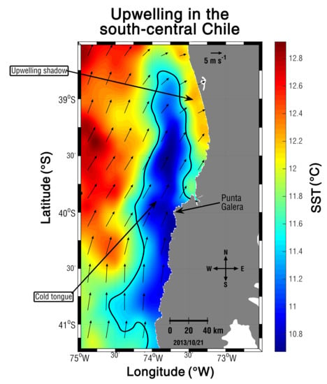
:The central and northern Chilean coasts are part of the Humboldt Current System, which sustains one of the largest fisheries in the world due to upwelling. There are several upwelling focal points along the Chilean coast; however, from a physical standpoint, the region between 39° and 41° S has not been studied in detail despite being one of the most productive zones for pelagic extraction in Chile. Here, we evaluated the seasonal variability of coastal upwelling off central-southern Chile using principally daily sea surface temperature (SST) and sea surface wind (SSW), and 8-day composite chlorophyll-a concentration between 2003 and 2017. Through the seasonal evaluation of the net surface heat flux and its relationship with the SST as well as daily SST variability, we determined the “maximum upwelling” on our area. The direction of surface winds is controlled throughout the year by the Southeast Pacific Subtropical Anticyclone, which produces a cold tongue and an upwelling shadow north of Punta Galera (40° S) in austral spring and summer. A cross-correlation analysis showed a decrease of SST follow the alongshore SSW with a lag of 2 days in the months favorable to the upwelling. However, the correlations were not as high as what would be expected, indicating that there is a large advection of waters from the south that could be related to the greater volume of subantarctic water present in the zone.
1. Introduction
The world’s most productive coastal biological zones and fisheries are found in the great upwelling systems of the California, Canary, Benguela, and Humboldt [1,2]. The Humboldt Current System (HCS), also known as the Chile–Peru Current, is located on the eastern border of the Southeast Pacific Subtropical Anticyclone (SPSA), and is bordered in the north by the Equatorial Current System and in the south by the South Pacific Current commonly known as the West Wind Drift [3,4]. This system supports Chile’s principal fisheries according to 2014 Food and Agriculture Organization’s statistics, including sardine and anchovy [5]. The HCS is driven principally by the SPSA, which controls winds along the coast [6,7]. During austral fall and winter, SPSA is located at low latitudes, with its center near 27–29° S, which makes the winds favorable for upwelling only in Chile’s northern region (18–28° S). In austral spring and summer, SPSA is located at middle latitudes, with its center near 30–33° S, which creates winds favorable for upwelling from the north to central-southern Chile (28–41° S) [8,9]. This generates transport of cold, oxygen-poor, high-nutrient water to the sea surface over the continental shelf [10].
Upwelling has been observed to be more intense in points and capes [10] and particularly strong in zones with wide and shallow continental shelves [1]. In Chile, several upwelling centers have been identified, of which some of the most significant are the Península de Mejillones (23° S), Punta Lengua de Vaca (30° S) [11], Punta Curaumilla (33° S), Punta Topocalma (34°10’ S), Punta Nugurne (35°57’ S), Punta Lavapié (37°15’ S), and Punta Galera (40° S) [12]. The continental shelf has a width that varies from 20 km in the north to 60 km in the central-southern zone (39–40° S) considering the 200 m isobath [13]. Although Punta Galera (Figure 1) has been cited as being an important Chilean upwelling zone, its synoptic and seasonal variability has not been studied in detail. Projections for the year 2100 in Chile under a moderately intense global change scenario show that the SPSA will move south, extending the duration of southerly winds along subtropical coasts [14]. Near 40° S, winds favorable for upwelling would stay for around two months more than they currently do [14], which would make this region one of Chile’s most important fisheries in the future, especially for the common sardine and anchovy [15].
The present study investigated seasonal variability of upwelling off central-southern Chile using sea surface temperature (SST), surface chlorophyll-a concentration (Chl-a), and sea surface wind (SSW) measurements obtained from different satellite sensors between 2003 and 2017. Punta Galera was found as an important upwelling site during spring and summer. During these seasons, the alongshore SSW causes a cold tongue and an upwelling shadow. This study improves understanding of coastal dynamics due to upwelling and serves as a base to establish possible changes due to different global warming scenarios.
2. Materials and Methods
2.1. Satellite Data: Sea Surface Temperature, Chlorophyll-a Concentration, and Sea Surface Winds
Daily SST was obtained from the web page https://coastwatch.pfeg.noaa.gov/erddap/griddap/jplMURSST41.html between 2003 and 2017 (15 years). These data come from MODIS and AMSR-E sensors aboard satellites Aqua and Terra, AVHRR-3 sensor aboard satellite NOAA-18, and WindSat sensor aboard the Coriolis satellite. SST data derived from a Multi-sensor Ultra-high Resolution (MUR) analysis was used. This product was obtained from 8 satellites objectively interpolate to level 4 (L4), with a 1 km spatial resolution [16]. MUR uses Multi-Resolution Variation Analysis (MRVA) to obtain an L4 product, which is based on a decomposition wavelet. The advantage of this product is that it combines all these satellites which have sensors of different characteristics. On the one hand, infrared sensors have an excellent spatial resolution of around 1 km and 4 to 8.8 km (AVHRR) and microwave sensors have a resolution of 25 km. The infrared sensors can offer a very high spatial resolution and the microwave sensors are less prone to be contaminated by cloudiness. In addition, the MRVA method uses different synoptic time scales that allow for the reconstruction of mesoscale features (e.g., the upwelling) and its “mesh-less” interpolation procedure prevents truncation of the geolocation data during gridding and binning of satellite samples. Therefore, the combination of several types of sensors and the interpolation method used allow us to obtain daily good quality images without major cloudiness contamination problems. More information regarding how to produce L4, procedures, quality control, and a description of the MRVA algorithm can be found at References [16,17]. These data have been successfully used to locate and track frontal structures, thus helping to better identify the scale of upwelling along the Peruvian coast [18] and central Chile [19,20]. Data of surface Chl-a (mg m−3) were obtained by satellite data derived from MODIS Aqua level 3 which are freely available on NASA’s website (https://oceancolor.gsfc.nasa.gov/cgi/l3) at a spatial resolution of 4 km and daily and 8-day composites for the same time period of SST. In most analyzes, we prefer to use 8-day composites instead of daily because in our study area there is a lot of contamination by clouds, especially in winter [12]. Chl-a were estimated using the OCI algorithm [21].
Magnitude and direction of daily SSW correspond to products developed by the French Research Institute for Exploitation of the Sea. These products were interpolated using the objective method and based on data from scatterometers aboard satellite QuikSCAT (SeaWind sensor) [22] and MetOP (ASCAT sensor) [23], both at a spatial resolution of 25 km. QuikSCAT data from January 2003 and October 2009 (the latter date is approximately when it stopped working) and by ASCAT between May 2007 (when it began operations) and December 2017. The information presented here is from products derived from ASCAT satellite and data obtained before October 2009 using linear regression between the two databases in which the independent variables were products derived from QuikSCAT. A fusion of the SSW components with monthly data using linear regression was used throughout the north-central Chilean coast with very high correlations, especially for the meridional component [7].
2.2. Methodology
To understand seasonality of SST, Chl-a, and SSW, monthly averages were obtained for the study period and later averaged for austral summer (January–March), autumn (April–June), winter (July–September), and spring (October–December). Each SSW field component was averaged in the study area and separated by season to establish the frequency of its magnitude and direction.
To evaluate upwelling, we conducted a preliminary analysis of the net surface heat flux (Qnet) and SST. Thus, when we analyzed seasonally the Qnet, we observed the highest values towards the coast (higher than 120 W m−2), during the austral spring–summer seasons (Figure 2a). A similar pattern was observed for Qnet for autumn–winter seasons but with values decreased by approximately 110 W m−2 (Figure 2b). According to this analysis, we should expect higher (lower) temperatures during spring–summer (autumn–winter) seasons, especially towards the coast. However, lower SST values were observed towards the coast during spring–summer seasons (Figure 2c). This would indicate that during spring–summer seasons there is an advective process that is cooling near the coast and that would be mainly due to the effect of upwelling. These characteristics must be observed when analyzing the spatial standard deviation of all the SST images (Figure 3). Thus, offshore we obtained the largest standard deviations congruent with the seasonal pattern of the Qnet. On the other hand, near the coast, we observed the smallest standard deviations owing to the seasonal pattern of the Qnet and the effect of the upwelling that diminishes the temperatures during spring–summer seasons (Figure 2c).
In order to evaluate the upwelling, we analyzed the response of the SST to the wind. To do this, we chose the area where the standard deviations of the SST were the smallest which should be the area of “maximum upwelling” (Figure 3, rectangle 1) and the area closest to Punta Galera (Figure 3, rectangle 2). In the first zone, we calculated the minimum daily SST which was then averaged (714 pixels) and in the second zone we computed the mean daily alongshore SSW which was later averaged (9 pixels). In this way, we obtained two-time series, one of SST and the other of the alongshore SSW. Then, we calculated the long-term monthly averages of the SST and the alongshore SSW. Then, based on the long-term monthly averages, we calculated the daily SST anomalies and daily alongshore SSW anomalies. Finally, a cross-correlation between the anomalies of both variables, considering a maximum lag of 10 days for each season and year, was computed. Therefore, we obtained a total of 60 correlations (15 correlations for each season).
On the other hand, to analyze the primary productivity response, we performed an analysis similar to that indicated above. In the area of “maximum upwelling” (rectangle 1 in Figure 3), we calculated the maximum daily and 8-day composites Chl-a which were then averaged (65 pixels). Chl-a lost by the effects of clouds were filled with linear interpolation (30.7% and 2.2% for daily and 8-day composites, respectively). As the time series did not have a normal distribution, we transformed it using the base 10 logarithm. Then, we calculated the long-term monthly averages of the daily and 8-day composite Chl-a and computed their respective anomalies. The previously obtained SST and alongshore SSW time series were averaged 8 days, and then calculated their long-term averages and their anomalies. Finally, a cross-correlation between the anomalies of Chl-a, SST, and alongshore SSW was computed.
3. Results
3.1. Seasonal Chlorophyll-a Concentration, Sea Surface Temperature, and Sea Surface Wind Cycle
Evolutions of 8-day composite Chl-a, daily SST, and daily alongshore SSW close to Punta Galera are presented in Figure 4. In general, the Chl-a did not have a very clear seasonal signal, its values fluctuated mostly around 0.3 and 2 mg m−3, and its peaks were more evident during spring and summer (Figure 4a). In contrast, the SST showed a clear seasonal pattern owing to the variation of solar radiation. The highest temperatures occurred during the summer where they reached between 17 and 18 °C while the lowest temperatures were in winter where they oscillated between 11 and 12 °C except for 2007 where it dropped to values lower than 10 °C (Figure 4b). In addition, the SST presented many pulses of low temperatures during spring and summer most likely related to the coastal upwelling. Like the SST, alongshore SSW also exhibited a clear seasonal pattern, but with many pulses throughout the entire time series (Figure 5c). The winds were favorable to the upwelling during spring and summer and their higher values fluctuated between 5 and 9 m s−1 while they were favorable to the downwelling during the winter where their higher intensities ranged between 5 and 6 m s−1.
3.2. Seasonal Variability of Sea Surface Temperature and Sea Surface Wind Fields
SSW in central-southern Chile changes direction and intensity throughout the year (Figure 5). In general, during austral summer, winds were parallel to the coast, coming from the southeast at 5 m s−1 and with lower SST on the continental shelf delimited with the black line (Figure 5a). During austral autumn, outside of the continental shelf, light winds came from the southeast to north of 40.5° S and from the northeast to south of the position mentioned previously, at a velocity less than 5 m s−1, while on the continental shelf velocities were between 2 and 0 m s−1 (Figure 5b). The pattern of SST in austral autumn was similar to that observed in summer, but with lower temperatures. For austral winter, the pattern of wind magnitude and direction was similar to that of autumn (Figure 5c). However, SST decreased drastically on and off the continental shelf, averaging around 11 °C, thus coastal-oceanic gradients seen in austral summer and autumn nearly disappeared. In austral spring, wind magnitude and direction changed drastically, with a velocity of approximately 5 m s−1, originating in the southeast (Figure 5d). SST values increased off the continental shelf, reaching 14 °C, and coastal-oceanic gradients began to establish themselves. Moreover, a cold tongue (~12 °C) towards the north of Punta Galera appeared on the continental shelf.
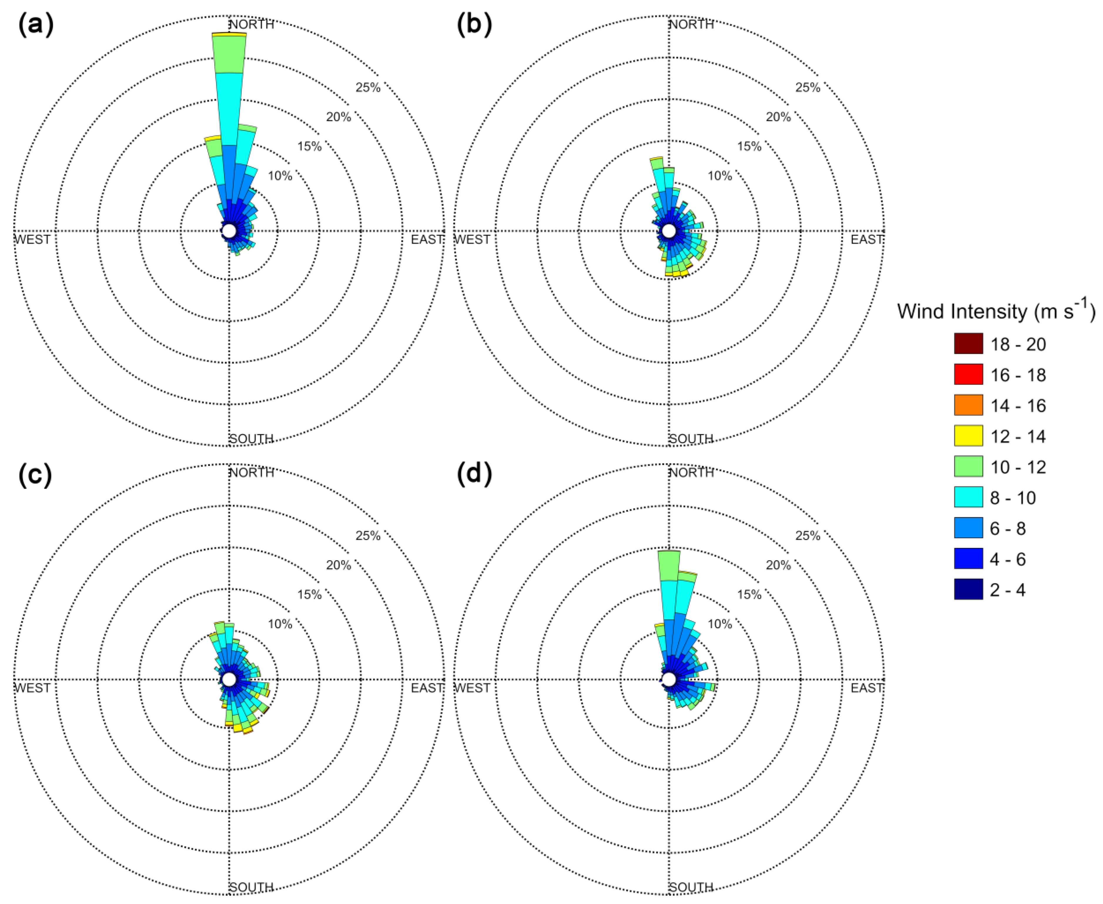
The frequency histogram of daily SSW magnitude and direction (Figure 6) shows a more accurate vision of the dominant winds in the zone, because they are not averaged by season. During austral summer, more than 60% of winds came from the southeast and southwest, with magnitudes between 6 and 10 m s−1 (Figure 6a). Magnitude and direction frequencies of SSW for austral autumn and winter were very similar. The greatest percentage of winds came from the northeast (approximately 18%–29%), with velocities fluctuating around 6–14 m s−1 (Figure 5c and Figure 6b). In austral spring, SSW showed a similar behavior to in summer; however, the direction of the predominant winds that came from the southeast and southwest was around 50% of the total (Figure 6d).
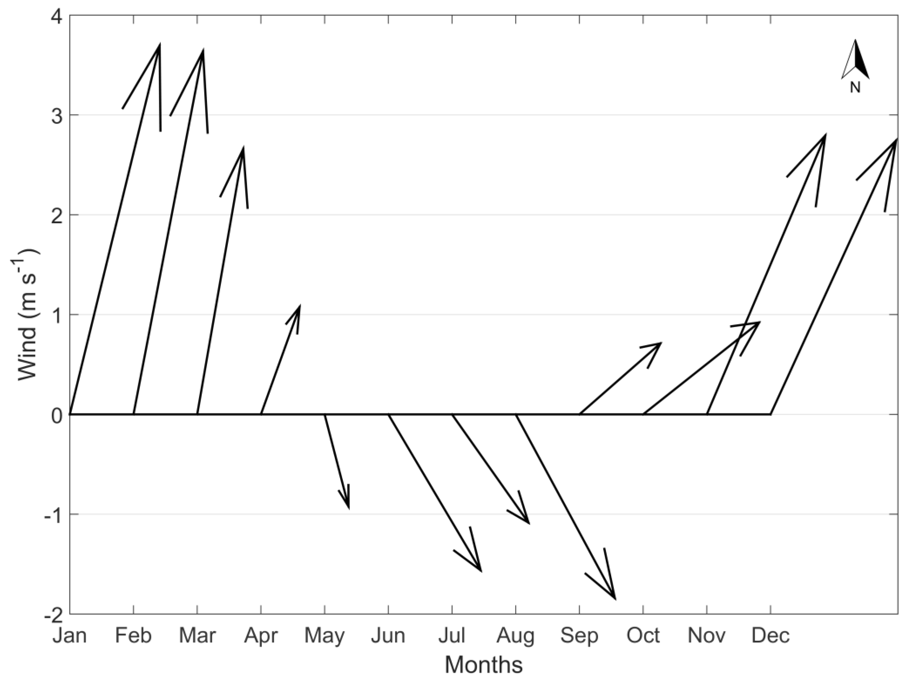
In order to evaluate the wind at Punta Galera, we obtained a stick plot of the long-term averages of the wind around ~40° S (Figure 7). Near Punta Galera, the wind seasonally came predominantly from the southwest between November and March with intensities that ranged between 3 and 4 m s−1. The months of April–May and September–October can be considered as transitional, where the wind intensity decreased between 1 and 1.5 m s−1 and had a weak meridional component. During the winter months (June–August), the winds intensified reaching values of 2 m s−1 but predominated from the northwest
3.3. Seasonal Variability of Surface Chlorophyll-a Concentration Field
The long-term average Chl-a for austral summer had the highest values along the continental shelf (~10 mg m−3), north of 40° S (Figure 8a). During austral autumn, the regional average decreased drastically, but stayed at relatively high levels (about 3 mg m−3) over the continental shelf, north of 40° S, and restricted towards shallower depths to the south (Figure 8b). During austral winter, relatively high levels (about 3 mg m−3) spread over the entire continental shelf. The contrast between the higher values near the coast and offshore was lower than in the other (Figure 8c). In austral spring, once again, high values were observed along the continental shelf, like those shown in summer, especially north of Punta Galera (~10 mg m−3) (Figure 8d).
3.4. Surface Wind Forcing Effects on Sea Surface Temperature and Surface Chlorophyll-a Concentration
Where there is upwelling of cold waters due to Ekman transport produced by winds favorable, it is to be expected that these effects would not be immediate. Thus, the cross-correlation between the daily alongshore SSW anomalies and daily SST anomalies close to Punta Galera showed the highest correlation at a 3-day lag, although it was low (R = −0.20) (Figure 9a). When the analysis was performed for each season, the correlations improved in the austral summer and spring, reaching −0.41 and −0.33, respectively, with an about 2-day lag (Table 1). However, in the austral autumn the correlations decreased (R = −0.20) with an around 4-day lag, and in the austral winter there was no correlation (Table 1).
When we performed a cross-correlation between 8-day composite Chl-a anomalies and the mean 8-day composite alongshore SSW anomalies, the correlation was low (R = 0.13) but significant with a 8-day lag. However, when 8-day composite Chl-a anomalies and 8-day composite SST anomalies, were cross-correlated the correlation improved to be −0.31, with a zero lag. To better explore the Chl-a delay time, we cross-correlated daily Chl-a anomalies and daily SST anomalies. The correlation was −0.27 at a 2-day lag (Figure 9b).
4. Discussion
We evaluated the upwelling at Punta Galera conducting a preliminary analysis of net surface heat flux and its relationship with SST as well as its daily variability throughout every year. This analysis helped us to determine the region of “maximum upwelling” associated with minimum SST during spring and summer. This region was located north of Punta Galera on the continental shelf, which agrees well with Figure 1b.
4.1. Seasonal Variability of Chlorophyll-a Concentration, Sea Surface Temperature, and Alongshore SSW Cycle at Punta Galera
The Chl-a in Punta Galera showed a seasonality during the year with higher concentrations at the beginning and end of each year (Figure 4a), like what occurs in the south and north of Chile with similar concentrations (e.g., [4,26]). The seasonality of the SST in Punta Galera is congruent with the annual variability of the net heat flux (Figure 2a,b). However, also there are advective processes (e.g., upwelling) that are less important than the sum of the terms that form the net heat flux as has been shown by Garcés-Vargas and Abarca-del-Río [27]. While interannual variability was not analyzed in this paper, the observed drop in SST during the second half of 2007 is associated with a strong La Niña (according to Oceanic Niño Index (https://origin.cpc.ncep.noaa.gov/products/analysis_monitoring/ensostuff/ONI_v5.php) similar decrease has also been observed in the temperature anomalies in the water column of a coastal station located further north (Concepción, 37° S) [28] and SST between 35° S and 38° S [29].
4.2. Seasonal Variability of Chlorophyll-a Concentration, Sea Surface Temperature, and Sea Surface Wind Fields
The highest values of Chl-a were found along the coast (Figure 8) with large fluctuations as shown near Punta Galera (Figure 4a) but with its highest concentrations in spring and summer and restricted to the continental shelf similar to that shown by Kämpf and Chapman [30], which is wider towards the north of Punta Galera than towards the south. The formation of a cold tongue that begins at this geographical point and is most evident during austral spring when the winds blow more alongshore and extend the upwelling area offshore to the continental shelf. This is very similar to what happens in the principal upwelling zones of Chile [2,12,29]. This cold tongue forms a thermal front around it and a small upwelling shadow that is very coastal and extends from the north of Punta Galera to approximately 39° S and is most clearly seen during austral spring (Figure 1b), similar to what occurs for example further north in Punta Lavapié (37° S) [31], Punta Lengua de Vaca [20] and Península Mejillones (23°42′ S, Antofagasta Bay) [32]. However, in the Península Mejillones, this shadow is permanent because the wind is always favorable for upwelling, which does not occur in our study area.
4.3. Effects of Sea Surface Wind Forcing on Sea Surface Temperature and Chlorophyll-a Concentration
The cross-correlation analysis between upwelling-favorable wind and SST also reaffirms the coupling between the two variables. For the entire period, there was a 3-day lag; however, the highest negative correlations were found in austral spring and summer with a 2-day lag (Table 1, summer and spring), while the lowest negative correlations were in austral autumn and winter with 4- and 3-day lags for autumn and winter, respectively (Table 1). In Antofagasta Bay (23°42’S), winds favorable to upwelling are permanent during the year, with a greater correlation in austral summer between the alongshore SSW and the reduction in SST with a 1-day lag [32]. Similarly, in Chile’s central region (32–36° S) where Punta Curaumilla (33° S) and Punta Topocalma (34°07’S) stand out, there is a delay of 3 days between both variables [10]. In addition, our results showed an inverse relationship between daily Chl-a anomalies and daily SST anomalies with a 2-day lag. This would indicate that decreasing (increasing) SST increases (decreases) the primary productivity within a reasonably short range.
The correlations between SST and the alongshore SSW were not as high as what would be expected indicating that other advective processes (e.g., horizontal advection) and atmospheric processes could explain the changes. In general, turbulent terms (latent and sensible heat flux, proportional to wind magnitude) should not change drastically between the coast and ocean because wind magnitude is similar (Figure 5) [33]. With respect to radiative terms, shortwave and longwave radiation also should not vary much because the former depends on cloud coverage (at the same latitude), which is similar in the region, and the latter is relatively constant [27]. It is probable that there is a large advection of waters from the south on the continental shelf that could be related to the greater volume of subantarctic water present in the zone [34].
The influence of the wind over the SST is in clear concordance with the movement of the SPSA. Thus, during austral summer and spring, the greater correlations between wind and temperature are due to a higher percentage of winds coming more from the south (Figure 6a,d), when the SPSA is more southern, intense, and farther from the continent [7]. On the other hand, during austral autumn and winter, the direction of the winds is not well marked (Figure 6b,c) and therefore the negative correlations were relatively low when SPSA is further north, weak, and close to the continent [7].
4.4. Potential Implications of Upwelling in Punta Galera due to Climate Change
Some authors mention that under the present climate change scenario with sustained increase in temperatures, the SPSA center would migrate further south in austral summer from 35° S (current situation) to 40° S (end of the 21st century) [14]. The displacement of SPSA towards the south has been observed in the last few decades [7,28], which would be currently causing a greater persistence of winds favorable to upwelling. If these projections are fulfilled, it could be expected that in Punta Galera the upwelling period will increase with the consequent decrease in SST and the stratification of the water column, which would contrast with the average situation globally.
5. Conclusions
The evaluation of the net surface heat and daily SST variability allowed us to find the “maximum upwelling” off central-southern Chile (39° S–41° S) showing that it is located north of Punta Galera over the continental shelf.
The direction of SSWs in the central-southern region of Chile is controlled during the year by the SPSA. During austral spring and summer, they migrate towards the south, causing alongshore SSW to promote upwelling (cold waters), high Chl-a and forming a coastal upwelling shadow (warmer waters) in the region.
The correlation analysis between the alongshore SSW and SST reaffirmed that Punta Galera is an important upwelling center off central-southern Chile, with a 2-day lag for the maximum negative correlation during austral spring and summer.
The need to measure currents in order to determine the horizontal advective terms and then improve the upwelling assessment through the SST as well as exploring its interannual variability is a major challenge for future research.
Author Contributions
A.P. and J.G.-V. conceived, designed the methodology, and wrote the paper; A.P., J.G.-V., F.O. and C.L. collected and processed the data and performed the analysis.
Funding
This study was financed by the CONICYT/FONDECYT (grant number: 1171171) and the Vicerrectoría de Investigación, Desarrollo y Creación Artística, Universidad Austral de Chile and partial funding was provided by CONICYT through the Program FONDAP, Project N° 15150003. C.L. was supported by the Millennium Nucleus Center for the Study of Multiple Drivers on Marine Socio-Ecological Systems (MUSELS) funded by MINECON NC12008.
Acknowledgments
We thank the anonymous reviewers for the constructive criticisms that helped to considerably improve the paper. Net surface heat flux product was provided by the WHOI OAFlux project (http://oaflux.whoi.edu) funded by the NOAA Climate Observations and Monitoring (COM) program. The Oceanic Niño Index was from NOAA Climate Prediction Center.
Conflicts of Interest
The authors declare no conflicts of interest.
References
- Patti, B.; Guisande, C.; Vergara, A.; Riveiro, I.; Maneiro, I.; Barreiro, A.; Bonanno, A.; Buscaino, G.; Cuttitta, A.; Basilone, G. Factors responsible for the differences in satellite-based chlorophyll a concentration between the major global upwelling areas. Estuar. Coast. Shelf Sci. 2008, 76, 775–786. [Google Scholar] [CrossRef]
- Carr, M.E.; Kearns, E.J. Production regimes in four Eastern Boundary Current systems. Deep Sea Res. Part Ii Top. Stud. Oceanogr. 2003, 50, 3199–3221. [Google Scholar] [CrossRef]
- Thiel, M.; Macaya, E.C.; Acuna, E.; Arntz, W.E.; Bastias, H.; Brokordt, K.; Camus, P.A.; Castilla, J.C.; Castro, L.R.; Cortes, M. The Humboldt Current System of northern and central Chile: Oceanographic processes, ecological interactions and socioeconomic feedback. Oceanogr. Mar. Biol. 2007, 45, 195–344. [Google Scholar]
- Morales, C.E.; Hormazabal, S.; Andrade, I.; Correa-Ramirez, M.A. Time-Space Variability of Chlorophyll-a and Associated Physical Variables within the Region off Central-Southern Chile. Remote Sens. Basel 2013, 5, 5550–5571. [Google Scholar] [CrossRef] [Green Version]
- FAO. El Estado Mundial de la Pesca y la Acuicultura 2016—Contribución a la Seguridad Alimentaria y la Nutrición Para Todos; Organización de las Naciones Unidas para la Alimentación y la Agricultura: Roma, Italia, 2016. [Google Scholar]
- Fuenzalida, R.; Schneider, W.; Garcés-Vargas, J.; Bravo, L. Satellite altimetry data reveal jet-like dynamics of the Humboldt Current. J. Geophys. Res. Ocean. 2008, 113. [Google Scholar] [CrossRef]
- Ancapichún, S.; Garcés-Vargas, J. Variability of the Southeast Pacific Subtropical Anticyclone and its impact on sea surface temperature off north-central Chile. Cienc. Mar. 2015, 41, 1–20. [Google Scholar] [CrossRef] [Green Version]
- Aguirre, C.; Pizarro, O.; Strub, P.T.; Garreaud, R.; Barth, J.A. Seasonal dynamics of the near-surface alongshore flow off central Chile. J. Geophys. Res. Ocean. 2012, 117. [Google Scholar] [CrossRef] [Green Version]
- Strub, P.T.; James, C.; Montecino, V.; Rutllant, J.A.; Blanco, J.L. Ocean circulation along the southern Chile transition region (38–46° S): Mean, seasonal and interannual variability, with a focus on 2014–2016. Prog. Oceanogr. 2019, 172. [Google Scholar] [CrossRef]
- Bello, M.; Barbieri, M.; Salinas, S.; Soto, L. Surgencia costera en la zona central de Chile, durante el ciclo El Niño-La Niña 1997–1999. In El Niño-La Niña 1997-2000. Sus Efectos en Chile; Avaria, S., Carrasco, J., Rutland, J., Yañez, E., Eds.; CONA: Valparaíso, Chile, 2004; pp. 77–94. [Google Scholar]
- Rutllant, J.; Montecino, V. Multiscale upwelling forcing cycles and biological response off north-central Chile. Rev. Chil. De Hist. Nat. 2002, 75, 217–231. [Google Scholar] [CrossRef] [Green Version]
- Letelier, J.; Pizarro, O.; Nuñez, S. Seasonal variability of coastal upwelling and the upwelling front off central Chile. J. Geophys. Res. Ocean. 2009, 114. [Google Scholar] [CrossRef] [Green Version]
- Völker, D.; Geersen, J.; Contreras-Reyes, E.; Sellanes, J.; Pantoja, S.; Rabbel, W.; Thorwart, M.; Reichert, C.; Block, M.; Weinrebe, W.R. Morphology and geology of the continental shelf and upper slope of southern Central Chile (33–43° S). Int. J. Earth Sci. 2014, 103, 1765–1787. [Google Scholar] [CrossRef]
- Garreaud, R.D.; Falvey, M. The coastal winds off western subtropical South America in future climate scenarios. Int. J. Climatol. 2008, 29, 543–554. [Google Scholar] [CrossRef]
- Gatica, C.; Arteaga, M.; Giacaman, J.; Ruiz, P. Tendencias en la biomasa de sardina común (Strangomera bentincki) y anchoveta (Engraulis ringens) en la zona centro-sur de Chile, entre 1991 y 2005. Investig. Mar. 2007, 35, 13–24. [Google Scholar] [CrossRef]
- Chin, T.M.; Vazquez-Cuervo, J.; Armstrong, E.M. A multi-scale high-resolution analysis of global sea surface temperature. Remote Sens. Environ. 2017, 200, 154–169. [Google Scholar] [CrossRef]
- Chin, T.M.; Vazquez, J.; Armstrong, E. Algorithm Theoretical Basis Document: A Multi-Scale, Hight-Resolution Analysis of Global Sea Surface Temperature, Version 1.3 ed.; Jet Propulsion Laboratory: Pasadena, CA, USA, 2013; p. 13.
- Vazquez-Cuervo, J.; Dewitte, B.; Chin, T.M.; Armstrong, E.M.; Purca, S.; Alburqueque, E. An analysis of SST gradients off the Peruvian Coast: The impact of going to higher resolution. Remote Sens. Environ. 2013, 131, 76–84. [Google Scholar] [CrossRef]
- Vazquez-Cuervo, J.; Torres, H.S.; Menemenlis, D.; Chin, T.; Armstrong, E.M. Relationship between SST gradients and upwelling off Peru and Chile: Model/satellite data analysis. Int. J. Remote Sens. 2017, 38, 6599–6622. [Google Scholar] [CrossRef]
- Bravo, L.; Ramos, M.; Astudillo, O.; Dewitte, B.; Goubanova, K. Seasonal variability of the Ekman transport and pumping in the upwelling system off central-northern Chile (~30° S) based on a high-resolution atmospheric regional model (WRF). Ocean Sci. 2016, 12, 1049–1065. [Google Scholar] [CrossRef]
- O’reilly, J. Ocean color chlorophyll a algorithms for SeaWiFS, OC2, and OC4: Version 4. Seawifs Postlaunch Calibration Valid. Anal. 2000, 3, 9–23. [Google Scholar]
- Piolle, J.F.; Bentamy, A. Quickscat Scatterometer Mean Wind Fileds Products User Manual; Department of Oceanography from Space (IFREMER): Plouzane, France, 2002. [Google Scholar]
- Bentamy, A.; Fillon, D.C. Gridded surface wind fields from Metop/ASCAT measurements. Int. J. Remote Sens. 2012, 33, 1729–1754. [Google Scholar] [CrossRef]
- Yu, L.; Jin, X.; Weller, R. Multidecade Global Flux Datasets from the Objectively Analyzed Air-sea Fluxes (OAFlux) Project: Latent and Sensible Heat Fluxes, Ocean Evaporation, and Related Surface Meteorological Variables; OAFlux Project Technical Report. OA-2008-01; Woods Hole Oceanographic Institution: Boston, MA, USA, 2008; Volume 74, p. 64. [Google Scholar]
- NGDC. 2-Minute Gridded Global Relief Data (ETOPO2 v2). Available online: https://www.ngdc.noaa.gov/mgg/global/etopo2.html (accessed on 30 January 2015).
- Yuras, G.; Ulloa, O.; Hormazábal, S. On the annual cycle of coastal and open ocean satellite chlorophyll off Chile (18–40° S). Geophys. Res. Lett. 2005, 32. [Google Scholar] [CrossRef]
- Garcés-Vargas, J.; Abarca-del-Río, R. The surface heat fluxes along the eastern Pacific coast from 10° N to 40° S. Aust. Meteorol. Ocean 2012, 62, 71–82. [Google Scholar]
- Schneider, W.; Donoso, D.; Garcés-Vargas, J.; Escribano, R. Water-column cooling and sea surface salinity increase in the upwelling region off central-south Chile driven by a poleward displacement of the South Pacific High. Prog. Oceanogr. 2017, 151, 38–48. [Google Scholar] [CrossRef]
- Kämpf, J.; Chapman, P. The Peruvian-Chilean Coastal Upwelling System. In Upwelling Systems of the World: A Scientific Journey to the Most Productive Marine Ecosystems; Springer International Publishing: Basel, Switzerland, 2016; pp. 161–201. [Google Scholar]
- Corredor-Acosta, A.; Morales, C.E.; Hormazabal, S.; Andrade, I.; Correa-Ramirez, M.A. Phytoplankton phenology in the coastal upwelling region off central-southern Chile (35–38° S): Time-space variability, coupling to environmental factors, and sources of uncertainty in the estimates. J. Geophys. Res. Ocean. 2015, 120, 813–831. [Google Scholar] [CrossRef]
- Paolini Cuadra, P.; Rodríguez, F.; Gallardo, C. Space-time characterization of Punta Lavapie upwelling system through SS NOAA/AVHRR images. Gayana (Concepción) 2004, 68, 459–465. [Google Scholar] [CrossRef]
- Piñones, A.; Castilla, J.C.; Guiñez, R.; Largier, J.L. Nearshore surface temperatures in Antofagasta Bay (Chile) and adjacent upwelling centers. Cienc. Mar. 2007, 33, 37–48. [Google Scholar] [CrossRef]
- Weller, R.A. Variability and trends in surface meteorology and air–sea fluxes at a site off northern Chile. J. Clim. 2015, 28, 3004–3023. [Google Scholar] [CrossRef]
- Nieto, K. Variabilidad Oceánica de Mesoescala en los Ecosistemas de Afloramiento de Chile y Canarias: Una comparación a partir de datos satelitales. Ph.D. Thesis, Universidad de Salamanca, Salamanca, Spain, 2009. [Google Scholar]
Figure 1.
Southeastern Pacific along continental Chile (a) and the study area (red box) off central-southern Chile (b), which includes sea surface temperature (SST, color, °C) from 21st October, 2013, which represents coastal upwelling in austral spring.
Figure 1.
Southeastern Pacific along continental Chile (a) and the study area (red box) off central-southern Chile (b), which includes sea surface temperature (SST, color, °C) from 21st October, 2013, which represents coastal upwelling in austral spring.

Figure 2.
Long-term averages of net surface heat flux (Qnet, W m−2) for (a) austral spring–summer and (b) autumn–winter, and (c) SST (°C) for spring–summer seasons. Qnet was obtained from WHOI Objectively Analyzed Air–Sea Fluxes [24] and their long-term averages correspond to values during 1984–2009.
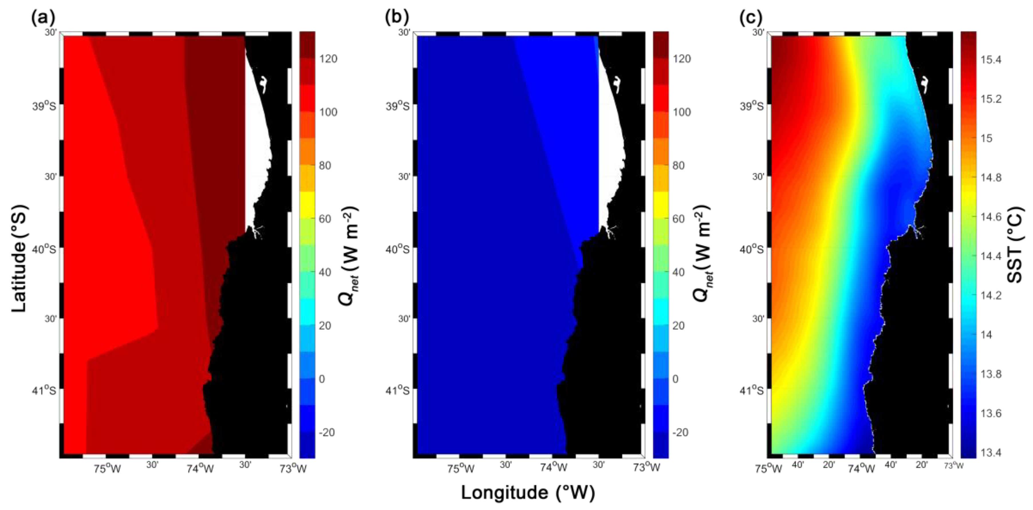
Figure 3.
Standard deviations of all SST images. The white rectangle 1 was used as a reference for SST and chlorophyll-a concentration (Chl-a) averages and the white rectangle 2 was used as a reference for alongshore sea surface wind (SSW) average.
Figure 3.
Standard deviations of all SST images. The white rectangle 1 was used as a reference for SST and chlorophyll-a concentration (Chl-a) averages and the white rectangle 2 was used as a reference for alongshore sea surface wind (SSW) average.

Figure 4.
Time series of maximum Chl-a (8-day composite) (a) and minimum SST (daily composite) (b) north of the Punta Galera (~39.25° S, Figure 3, rectangle white 1) and (c) mean alongshore SSW (daily) closest to Punta Galera (~40° S, Figure 3, rectangle white 2).
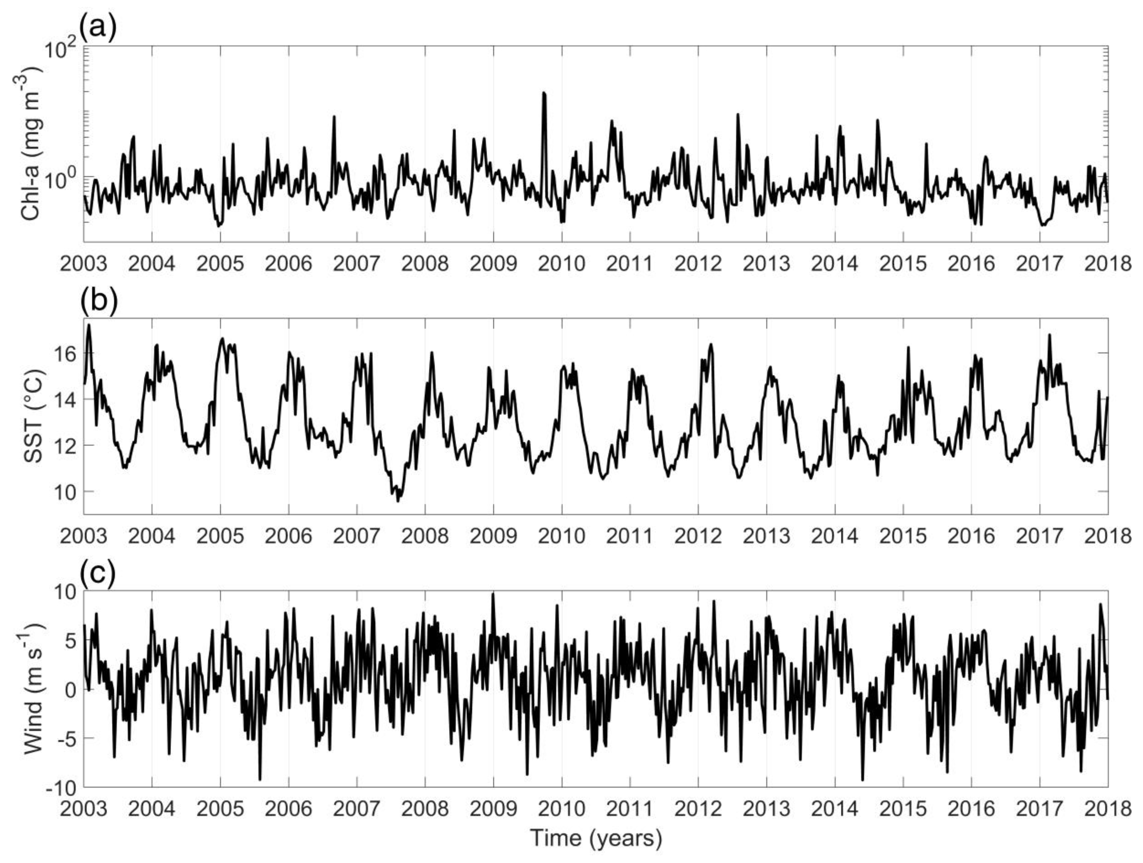
Figure 5.
Long-term averages of SST (color, °C) and SSW (black vectors, m s−1): austral summer (a), autumn (b), winter (c), and spring (d). At the bottom of each panel is an arrow indicating the wind scale. The boundary of the continental shelf is indicated with the 200 m isobath (black lines are for summer, autumn, and spring, and white lines are for winter) and was obtained from ETOPO2 v2 [25].
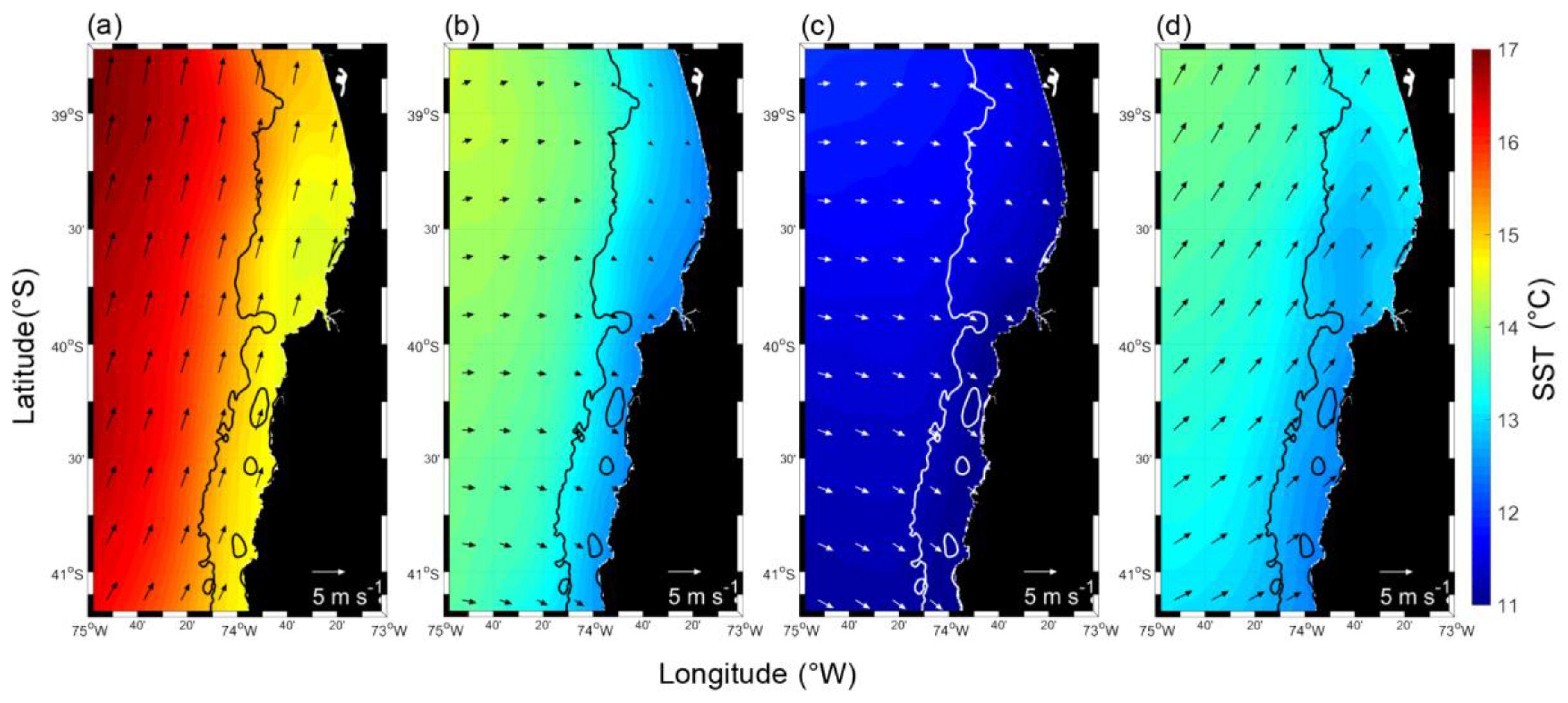
Figure 6.
Frequency histogram of daily surface wind magnitude and direction for the study area: austral summer (a), autumn (b), winter (c), and spring (d).
Figure 6.
Frequency histogram of daily surface wind magnitude and direction for the study area: austral summer (a), autumn (b), winter (c), and spring (d).

Figure 7.
Stick plot of the long-term averages of the wind closest to Punta Galera (~40° S, Figure 3, white rectangle 2).
Figure 7.
Stick plot of the long-term averages of the wind closest to Punta Galera (~40° S, Figure 3, white rectangle 2).

Figure 8.
Long-term average of Chl-a (color, mg m−3): austral summer (a), autumn (b), winter (c), and spring (d). The boundary of the continental shelf is indicated with the a 200 m isobath (black line) and was obtained from ETOPO2v2 [25].
Figure 8.
Long-term average of Chl-a (color, mg m−3): austral summer (a), autumn (b), winter (c), and spring (d). The boundary of the continental shelf is indicated with the a 200 m isobath (black line) and was obtained from ETOPO2v2 [25].
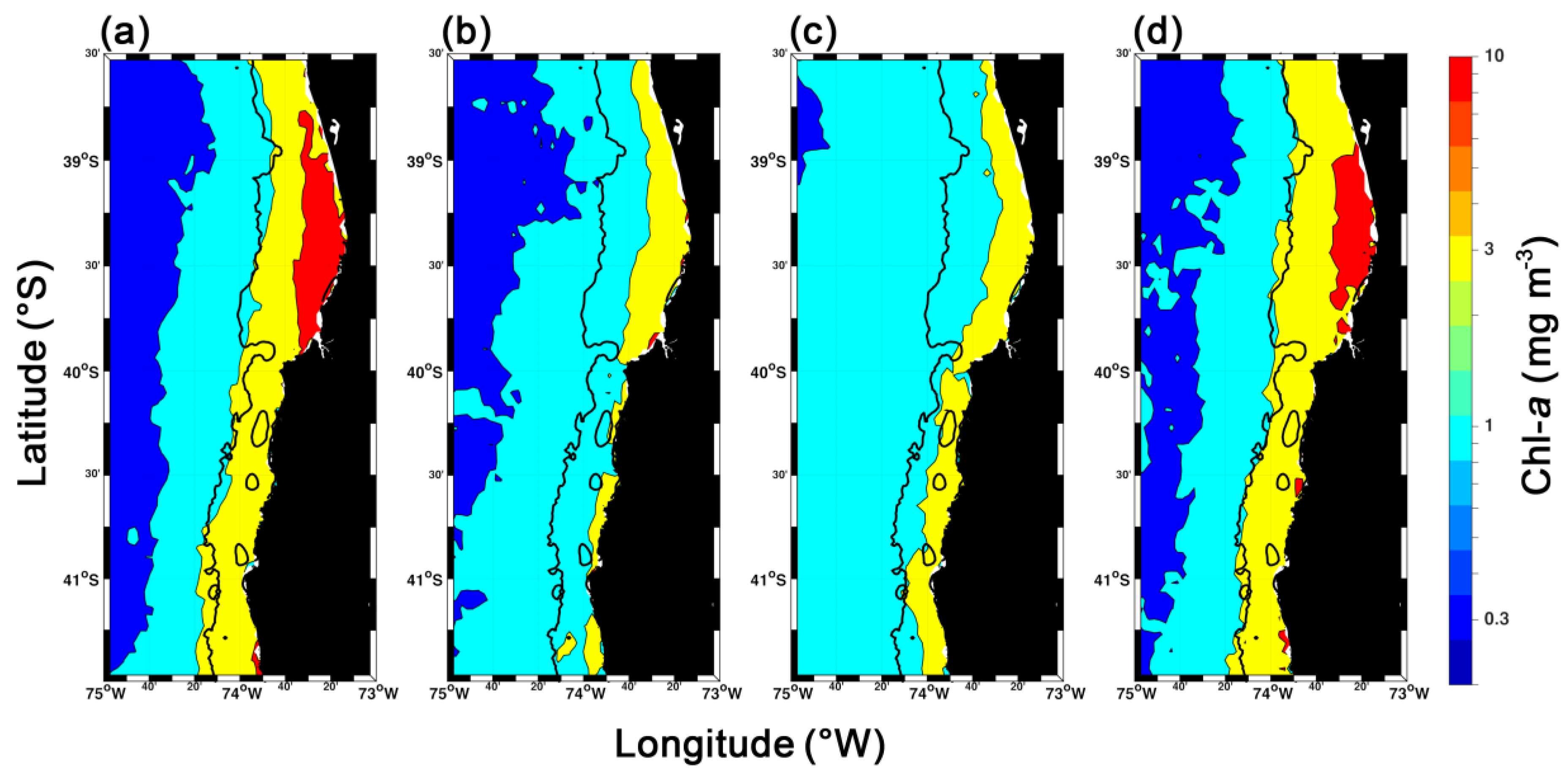
Figure 9.
Cross-correlation between daily SST anomalies and daily alongshore SSW anomalies (a) and daily SST anomalies and daily Chl-a anomalies (b). SST and Chl-a correspond to north of the Punta Galera (~39.25° S, Figure 3, rectangle white 1) and alongshore SSW correspond to the area closest to Punta Galera (~40° S, Figure 3, rectangle white 2). The blue lines in (a,b) shows the upper and lower confidence bound (95% confidence level).


Table 1.
Cross-correlation between daily SST anomalies north of the Punta Galera (~39.25° S, Figure 3, rectangle white 1) and alongshore SSW daily anomalies closest to Punta Galera (~40° S, Figure 3, rectangle white 2), per year and season.
| Summer | Autumn | Winter | Spring | |||||
|---|---|---|---|---|---|---|---|---|
| Year | Corr. | Lag (days) | Corr. | Lag (days) | Corr. | Lag (days) | Corr. | Lag (days) |
| 2003 | −0.59 | 2 | 0.34 | 1 | 0.29 | 1 | −0.004 1 | 3 1 |
| 2004 | −0.55 | 1 | −0.22 | 7 | 0.22 | 2 | 0.23 | 5 |
| 2005 | −0.45 | 2 | 0.36 | 0 | −0.21 | 6 | −0.36 | 3 |
| 2006 | −0.53 | 2 | −0.32 | 4 | −0.19 | 5 | −0.23 | 3 |
| 2007 | −0.43 | 3 | −0.17 1 | 5 1 | −0.12 1 | 6 1 | −0.46 | 1 |
| 2008 | −0.15 1 | 5 1 | −0.28 | 2 | 0.46 | 2 | −0.14 1 | 2 1 |
| 2009 | −0.27 | 1 | 0.18 1 | 0 1 | −0.38 | 2 | −0.42 | 2 |
| 2010 | −0.21 | 1 | 0.18 1 | 0 1 | −0.15 1 | 4 1 | −0.34 | 4 |
| 2011 | −0.51 | 1 | −0.4 | 5 | 0.06 1 | 1 1 | −0.34 | 2 |
| 2012 | −0.39 | 3 | −0.45 | 4 | −0.26 | 7 | −0.37 | 4 |
| 2013 | −0.27 | 3 | −0.31 | 10 | −0.32 | 4 | −0.52 | 0 |
| 2014 | −0.35 | 4 | −0.28 | 0 | 0.29 | 1 | −0.48 | 2 |
| 2015 | −0.56 | 0 | −0.47 | 2 | 0.3 | 0 | −0.5 | 1 |
| 2016 | −0.36 | 3 | −0.23 | 10 | 0.2 | 0 | −0.23 | 0 |
| 2017 | −0.2 | 4 | 0.16 1 | 6 1 | −0.19 1 | 5 1 | −0.28 | 0 |
| Mean 2 | −0.405 | 2.1 | −0.21 | 4.1 | 0.04 | 2.7 | −0.33 | 2.1 |
1 It is not a significant value (95% significance level). 2 Mean does not include non-significant values.
© 2019 by the authors. Licensee MDPI, Basel, Switzerland. This article is an open access article distributed under the terms and conditions of the Creative Commons Attribution (CC BY) license (http://creativecommons.org/licenses/by/4.0/).
Share and Cite
MDPI and ACS Style
Pinochet, A.; Garcés-Vargas, J.; Lara, C.; Olguín, F. Seasonal Variability of Upwelling off Central-Southern Chile. Remote Sens. 2019, 11, 1737. https://doi.org/10.3390/rs11151737
AMA Style
Pinochet A, Garcés-Vargas J, Lara C, Olguín F. Seasonal Variability of Upwelling off Central-Southern Chile. Remote Sensing. 2019; 11(15):1737. https://doi.org/10.3390/rs11151737
Chicago/Turabian StylePinochet, Andre, José Garcés-Vargas, Carlos Lara, and Francisco Olguín. 2019. "Seasonal Variability of Upwelling off Central-Southern Chile" Remote Sensing 11, no. 15: 1737. https://doi.org/10.3390/rs11151737
Note that from the first issue of 2016, this journal uses article numbers instead of page numbers. See further details here.