Progressive Cascaded Convolutional Neural Networks for Single Tree Detection with Google Earth Imagery


College of Computer Science and Technology, Zhejiang University of Technology, Hangzhou 310023, China
*
Author to whom correspondence should be addressed.
Remote Sens. 2019, 11(15), 1786; https://doi.org/10.3390/rs11151786
Submission received: 16 May 2019
/
Revised: 9 July 2019
/
Accepted: 19 July 2019
/
Published: 30 July 2019
(This article belongs to the Special Issue Advances in Active Remote Sensing of Forests)
Abstract
:High-resolution remote sensing images can not only help forestry administrative departments achieve high-precision forest resource surveys, wood yield estimations and forest mapping but also provide decision-making support for urban greening projects. Many scholars have studied ways to detect single trees from remote sensing images and proposed many detection methods. However, the existing single tree detection methods have many errors of commission and omission in complex scenes, close values on the digital data of the image for background and trees, unclear canopy contour and abnormal shape caused by illumination shadows. To solve these problems, this paper presents progressive cascaded convolutional neural networks for single tree detection with Google Earth imagery and adopts three progressive classification branches to train and detect tree samples with different classification difficulties. In this method, the feature extraction modules of three CNN networks are progressively cascaded, and the network layer in the branches determined whether to filter the samples and feed back to the feature extraction module to improve the precision of single tree detection. In addition, the mechanism of two-phase training is used to improve the efficiency of model training. To verify the validity and practicability of our method, three forest plots located in Hangzhou City, China, Phang Nga Province, Thailand and Florida, USA were selected as test areas, and the tree detection results of different methods, including the region-growing, template-matching, convolutional neural network and our progressive cascaded convolutional neural network, are presented. The results indicate that our method has the best detection performance. Our method not only has higher precision and recall but also has good robustness to forest scenes with different complexity levels. The F1 measure analysis in the three plots was 81.0%, which is improved by 14.5%, 18.9% and 5.0%, respectively, compared with other existing methods.
1. Introduction
With the development of remote sensing technology, there is a growing demand for the accurate detection of single trees based on high-resolution remote sensing images. Single tree detection is useful for forest management, afforestation and utilisation of forest resources. Single tree detection technology is a cross-research field of relevance for computer vision, photogrammetry and remote sensing fields and has become a hot topic in recent years [1,2]. Tree detection methods based on remote sensing images can be divided into two categories: pixel-based tree detection methods and object-based tree detection methods.
Early tree detection methods with remote sensing images are usually based on pixels. The most commonly used pixel-based method is the local-maximum method [3,4]. This kind of method usually extracts the maximum value of the local area as the centre of a tree, combined with the region-growing method, watershed segmentation method and other methods to detect single trees. For example, Novotny et al. [5] proposed a local-maximum method with a variable window size and used the region-growing method to detect trees. Culvenor [6] proposed a method based on image texture information to detect a single tree. They believed that the tree canopy vertex is a maximum value in the image, while the surrounding points are smaller. Therefore, they continued expanding from the maximum point to the surrounding points and stopped expanding once the value started to rise. This method does not require defining window size parameters as opposed to finding local maximum values. Hirschmugl et al. [7] proposed an algorithm to find the crown centre by eliminating non-crown regions before using the Levenberg–Marquardt algorithm (LMA), based on the comparison of existing crown centre acquisition methods. Pouliot et al. [8] designed an adaptive multi-scale single tree detection method. First, they selected the best Gaussian smoothing parameters according to the relationship between the number of local maximum values and the value of the Gaussian smoothing parameters, and then used the extracted local maximum points as a single tree through the adaptive window size. Because these local-maximum methods cannot be classified according to the overall features of trees, the accuracy of selecting seed points in a complex background will also be reduced, thus affecting the accuracy of single tree detection. In addition, the template-matching method [9,10,11] is also a pixel-based method, which uses the template of a tree to calculate the area with the same size as the area in the image successively and calculates the sum of squared errors of all the pixel points. However, this method cannot match the area with which the trees are located in a crowded manner, and the canopies often overlap.
The object-based tree detection method can better reflect the overall features of trees and improve the accuracy of tree detection by incorporating a machine learning algorithm. Hellesen et al. [12] proposed combining an object-based image analysis method with a classification tree algorithm to find the best classification features to distinguish shrubs, trees and background grasslands. When LiDAR-derived data were used as auxiliary information, the classification accuracy of object-based CIR orthographic image analysis was significantly improved. Laliberte et al. [13] proposed a method combining image segmentation and object-based classification to monitor the changes of vegetation over time, combining spectral and spatial image information, which is very close to the way that humans intuitively interpret information from aerial photographs. In addition, the multi-scale analysis combined with the hierarchical segmentation method is effective in the ecological sense, and the shrub density can be determined in the coarse-level classification. Salim et al. [14] used a method of scale-invariant feature transform (SIFT) to extract the key points of palm trees and put them into the extreme learning machine (ELM) for learning classification, thereby realising the detection of a single tree. However, SIFT selects the features of several key points in the sample, which is slightly less accurate than the global feature method based on RGB. Lin et al. [15] proposed a method of automatic training and data selection. They used the overall colour, texture, entropy and other visual features of trees in aerial images to train a pixel-level classifier, and the training process and data selection were based on two-level clustering. However, this method requires manually specifying extracted features and setting limits for the corresponding parameters for different scenarios, and it is difficult to detect a single tree accurately without prior knowledge.
In recent years, with the increasing application of the convolutional neural network (CNN) algorithm in target recognition and image classification of computer vision, researchers have also begun to apply CNN to tree detection of remote sensing images [16,17,18,19,20] to solve the problems in traditional single tree detection methods. For example, the robustness of the seed point selection or template-matching method in the pixel-based detection approaches in complex scenarios is low, and the feature parameters of different scenarios need to be specified by prior knowledge in the object-based detection methods. The CNN does not require prior knowledge of artificially specified features and can continuously learn in-depth features based on numerous images. The conventional single tree detection algorithm first extracts the features and then conducts the classifier training, while the CNN network combines these two separate processes; thus, the bottom, colour, contour and other local low-level features are gradually abstracted to the high-level features. Li et al. [21] applied the method based on a deep learning convolutional neural network to the detection of densely planted oil palm trees in Malaysia. Overall, 96% of the manually marked trees in the test area were correctly detected. Emilio et al. [22] proposed a CNN-based Ziziphus lotus shrub detection method with Google Earth imagery as the data source and achieved a better detection result than the other single tree detection methods. In addition, other CNN-based algorithms such as Faster-RCNN [23] and YOLO (You Only Look Once) [24] can also be used to detect target objects, but if the resolution of the image is not high enough, such methods will miss some small trees. In general, tree detection methods based on convolutional neural networks are effective when the trees are similar in size and the scene is simple, but its robustness is not ideal for scenarios with complex backgrounds and diverse trees, such as trees and shrubs growing together, different tree species, etc. Since the convolutional neural network can only be trained for all candidate tree samples, most errors of commission and omission occur in the hard-to-classify samples with similar colour to background, unclear canopy contour and abnormal shape caused by illumination shadows. To improve the precision of the recognition of hard-to-classify samples, a progressive cascaded convolutional neural network for the single-tree detection method is proposed in this paper. Tree samples of different classification difficulties are trained and tested by different classification branches. The method cascades through three convolution layers and pooling layers based on the LeNet variant network and then forms the feature extraction modules. The remaining network layers are used as classification branch modules. By allowing the data sample to pass through each classification branch, it is fed back to the feature extraction module to determine whether it needs to be progressed into the next classification branch to extract the deeper features. As a result, the method can quickly identify parts of the low-level branches that are either clearly trees or not trees, and the high-level branches can extract more features of the sample to handle hard-to-classify samples. In addition, we propose a two-phase training and a method of feature maps that are partly shared to improve the efficiency of model training. This paper is not the first object detection method using cascaded convolutional neural networks for images [25,26], but the model designed for single tree detection in this study has many advantages, for example, the later classification branches can directly use the feature graph from the previous classification branch, avoiding the recalculation of the feature maps from the original diagram layer by layer; moreover, the network can be combined to train parameters in a global optimisation way, whereas previous cascading networks are basically independent networks.
2. Study Areas
This paper uses the highly accessible Google Earth imagery data [27] compared to expensive, private, and difficult to obtain satellite remote sensing images. In this study, three test areas were selected, located in Thailand, USA and China. Figure 1 shows a schematic of the location of the test areas. The reference tree is defined in the yellow line because trees outside the yellow line cannot be judged by human eyes. Test Area 1 is the palm tree plantation scenario in Phang Nga, Thailand, located at east longitude and north latitude. Palm trees are an important economic crop in Thailand, and more than 800 reference trees in Test Area 1 were selected. Test Area 2 is a complex greening area in Hangzhou, China, located at east longitude and north latitude. This area not only has different tree species but also rivers, buildings, roads, etc., and 254 reference trees were selected in Test Area 2. Test Area 3 is a real forest area in Florida, USA, located at west longitude and north latitude. In total, 261 reference trees were selected in Test Area 3. For a real forest area, the single tree detection is the basis for more effective forest management, thus we also tested our algorithm in Test Area 3.
3. Methods
Many training samples were used to train the model, and the classification precision was calculated by test samples. The main parameters in the network (such as the number of convolution kernels per convolution layer and the number of hidden layer units per full-connect layer) needed to be continuously adjusted by the global precision of the test samples. By adjusting the parameters, the best progressive cascaded detection model could be obtained. The detection model was adopted to detect trees on Google Earth imagery.
3.1. Overall Process
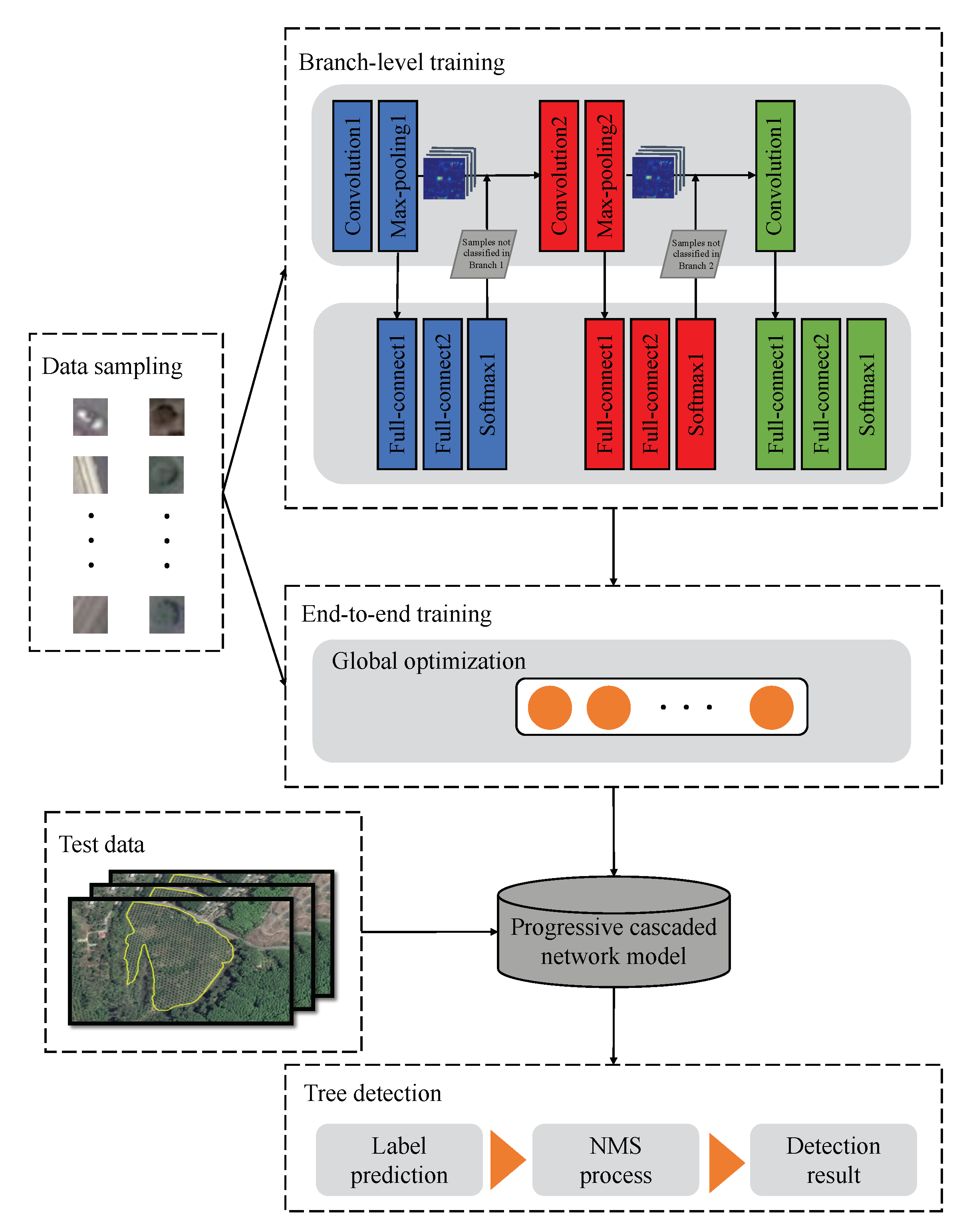
The overall process of single tree detection in this paper is shown in Figure 2, which mainly includes the steps of data sampling, branch-level training for cascaded networks, end-to-end training, and tree detection using cascaded networks.
- (1)
- Data Sampling: We collected image samples from Google Earth imagery. Many samples were manually labelled, and data argumentation, also called data transformation, which was used to artificially increase the number of samples in the training set by applying specific transformations (such as rotation, flipping, panning, cropping, or changing brightness) to the input image, generated 6000 samples, including 5280 training samples and 720 test samples, for training the progressive cascaded convolutional neural network and calculating classification precision. The samples included 3000 positive samples and 3000 negative samples.
- (2)
- Branch-level Training: When branch-level training was performed on the training data, training for each classification branch could initialise the weights of the classification branch, and each branch completed the training and detection of samples of different difficulties.
- (3)
- End-to-End Training: The global optimisation of the parameters of the entire network was conducted. Through the gradient descent optimisation method, training samples continuously adjusted the parameters to obtain the best cascaded CNN model.
- (4)
- Tree Detection: We predicted the label of all samples in the detection image set collected by the sliding window through the progressive cascaded detection model, that is, determining whether it is a tree. Finally, the non-maximum suppression (NMS) algorithm merged the prediction window corresponding to the same tree to obtain the final tree detection result.
3.2. Data Sampling
To obtain the detector with the best detection effect, the samples required for training should be abundant. Because of the wide variety of trees in remote sensing images, such as isolated trees, stuck trees, larger trees, smaller trees, and trees with illuminated shadows, various types of tree samples also needed to be covered as much as possible. In total, 1500 tree samples were labelled, including 750 positive samples and 750 negative samples. At the same time, the data argumentation method of rotation and folding was used to expand the labelled samples to 6000 training and validation samples. All of the trees of different sizes were scaled to the same size () before training. A larger dataset could be constructed from a small number of initial samples with data argumentation. Using different data argumentation methods to increase the size of the training dataset increased the generalisation performance of the model, reduced the risk of overfitting, and made the CNN model more robust to the scale, brightness, and geometric distortions [28,29].
The data sampled by the experiment are shown in Figure 3.
3.3. Training for Progressive Cascaded Convolutional Neural Networks
3.3.1. CNN-Based Progressive Cascaded Networks
The design of each individual classification branch in the model was based on the classic CNN model LeNet-5, as shown in Figure 4.
In this study, the structure of the progressive cascaded convolution neural network was designed, as shown in Figure 5. The tree samples in this network were divided into image batches and input into each branch network in turn. The last layer of each branch network was the SoftMax layer, which produced a classification probability between 0 and 1 after the training of the corresponding branch. The larger the value of probability was, the higher the confidence of the tree was, and vice versa. Meanwhile, we set a set of threshold intervals of positive and negative samples through grid search, that is, the classification probability of the sample in the former branch network was within the threshold intervals, so that the tree samples could be progressively moved to the next branch network to extract deeper tree features. If the classification probability were greater than the positive sample threshold, it would be labeled as an easy-to-classify positive sample when being filtered. Similarly, the classification probability less than the negative sample threshold was labeled as an easy-to-classify negative sample. It can be seen from the blue dotted line diagram that, for example, the first branch network has a lower probability of output for most samples, which differ greatly from the real tree colour or have no tree contour, thus it is labeled as the most easy-to-classify negative sample of the first branch and then feeds back to the feature map set extracted from the branch for elimination. Similarly, the red dotted line diagram graph shows that the sample output, which is most easily classified as tree, remains a higher probability, thus it is labeled as the most easy-to-classify positive sample of the first branch and eliminated. The remaining hard-to-classify samples are progressively input to the second branch network to extract deeper features. In the second branch network, interference background such as roads and buildings are labeled as more easy-to-classify negative samples and feed back to the feature graph set extracted from the branches for elimination. The third branch can be dedicated to training the most hard-to-classify samples.
Such a mechanism has two advantages: many easy-to-classify samples are detected in the previous classification branch, and the number of samples required for subsequent networks to be trained is reduced, which can greatly improve the computational efficiency of the network. Each classification branch can be trained to detect tree targets of different levels of difficulty, rather than being trained for all samples each time. Moreover, the network cannot proficiently learn all the features of hard-to-classify samples. Ultimately, when three different networks work together, the entire network can be made more effective.
The number of samples in each image batch in our training process is N. The model has K branches and a training dataset , wherein represents the ith sample in an image batch on the jth branch and represents the label corresponding to the ith sample in the image batch on the jth branch. The samples of each classification branch for the image batch filter corresponding difficulty are divided into two cases, as shown in Equations (1) and (2):
- (1)
- When the probability outputted by the branch is greater than the branch positive sample threshold, it is processed as a positive sample corresponding to the degree of difficulty.
- (2)
- When the probability outputted by the branch is less than the branch negative sample threshold, it is processed as a negative sample corresponding to the degree of difficulty.
Accordingly, the sample filtered by each branch is used as feedback into the feature map set in the feature extraction module. The feature map of the training dataset is , where represents the corresponding feature map of the ith sample on the jth branch after feature extraction. The feedback process is shown in Equation (3).
The dotted frame of the network structure diagram obtained is mainly a feature extraction module composed of a convolution layer and pooling layer in the three branches, and the following dotted frame is mainly a classification branch module composed of other network layers in the three branches. An additional advantage of this cascaded network is that the feature maps are partly shared. Because the main module and classification branch module of the extraction feature are connected through the same cascaded network, the feature map obtained by extracting the feature can not only be fed into the classification branch module to obtain the classification probability to filter a hard-to-classify vs. an easy-to-classify, but also progress into the next classification branch to extract deeper features, avoiding the recalculation of the original feature map.
3.3.2. Branch-Level Training
Our cascaded network training process uses a two-phase training, including branch-level training and end-to-end training. The first phase is important because it can significantly accelerate the convergence of the subsequent training, which is mainly reflected in two aspects. First, the subsequent classification branch takes advantage of the feature maps extracted from the previous network, resulting in rapid convergence. Secondly, for end-to-end training, branch-level training can initialise parameters in the cascaded networks. Therefore, the network parameters only need to be fine-tuned when the method is training globally.
In branch-level training, we train each classification branch as a separate model. When the training of a classification branch causes the accuracy to reach a certain threshold, the training ends. The corresponding positive and negative sample thresholds are selected to remove the easy-to-classify samples, and these easy-to-classify samples are not entered into the next classification branch. Correspondingly, hard-to-classify samples are input into the next network for feature extraction. In Figure 6, there are several examples of hard-to-classify samples, to the left of which is the convolutional neural network model that identifies the wrong positive samples, and to the right are negative samples. It is worth mentioning that the accuracy threshold of the first classification branch is not very high because the early branch of the network only acts as a filter. In the end, the three classification branches use different calibration training sets to train in turn.
The gradient descent optimisation for training is generally based on the principle of minimising the loss of predictive values. Let x and y represent the input image and the corresponding output category label, respectively, and the minimised average loss of iterative training can be defined as the following formula [26]:
where N is the amount of data in the mini-batch in each iteration, I is the sequence number in the image batch, F is the predictive output of the network determined by the current parameter , R is the weight attenuation, and L is the loss function, which is used to measure the difference between the output category of the last layer and the ground truth.
3.3.3. End-To-End Training
At the end of branch-level training, end-to-end network training is conducted to optimise all classification branches at the same time. At this point, all data streams in the classification branch are the same, no sample removal is required, and global parameters are optimised directly from end-to-end, as shown in Figure 7.
The advantage of two-phase training versus direct training is that direct training is interrupted after each round of training, such as threshold judgement and sample elimination. When the image batch passes through a classification branch, it results in the inability to focus on the benefits of the GPU, which is processing-intensive computing at each iteration of training; thus, the direct training has a huge amount of time overhead. In the experiment, we used Intel® Xeon® CPU E5649 (2.53 GHz), and the GPU was NVIDIA Quadro 2000, which contains a total of 5280 training samples, and a full training time took nearly 30 h.
To avoid frequent interruptions, the first phase for each classification branch of the two-phase training performs as separate training, so that each classification branch only needs to centralise iteration calculations for its own separate branches, and the GPU can accelerate to calculate thresholds and eliminate samples after each branch is trained. The feature maps generated by the intermediate process are then input into the next classification branch for calculation. After the first phase of training, all networks save their own parameters and compute the flow chart for using in the second phase. In the second stage of end-to-end training, no interruption operation is required, and, when training, it is only necessary to fine-tune the parameters on the basis of the first phase, which greatly improves the efficiency of the training. The whole process is equivalent to training four separate network structures. The time complexity does not have explosive growth, and the training takes approximately one hour.
3.4. Single-Tree Detection
After obtaining the trained progressive cascaded convolutional neural network model, the samples need to be collected from the test image with the help of sliding window technology, as shown in Figure 8 below. The step length of the sliding window (the moving distance of the sliding window in each step) has a significant impact on the final tree detection results. If the step length is too large, many trees will be missed without being detected. If the step length is too small, the same tree target may be detected repeatedly. Moreover, due to the increase in the number of detections in the image, the label prediction process will become very slow and inefficient. Based on our experiment, it is more appropriate to set the step length to 2 pixels during the detection process. The samples obtained by sliding window technology are classified and predicted using a progressive cascaded model, and whether it is a tree or not is judged according to the classification probability of the network output.
The scale of sliding windows is changed when collecting samples because the shape and scale of trees vary in complex scenarios. The scale of the same sliding window can also have an important effect on the detection results. Different levels of complexity of the scene also need to have different scale changes, for example, in a large area of sparse planting forests, where the sizes of the trees are relatively close, the required scale may be relatively fixed, while, in complex forests, the span of tree sizes is relatively large, thus the range of the sliding window scale needs to be larger. Because of the small step length and the scale change of the sliding window, a reference tree may correspond to the prediction label of multiple sliding windows, at which point all the prediction labels are sorted in descending order by classification probability, starting from the sliding window of the first prediction label to calculate the overlapping area with the remaining sliding window. These redundant windows are removed when the overlapping area exceeds a certain threshold; then, the redundant window of the sliding window with the second forecast label is removed, and this process is repeated until the last window, the redundant window, is removed, as shown in Figure 9. For example, the three reference trees in the right rectangular bounding boxes correspond to the predictive labels of 2, 3, and 2 sliding windows. The eight classification probabilities of the prediction labels for the three reference trees are 0.95, 0.90, 0.85, 0.84, 0.78, 0.68 and 0.45. The overlapping area of the sliding window with a prediction label of 0.78 and the window with a prediction label of 0.90 exceed the threshold value, thus the label of 0.78 is removed. The prediction label for the first reference tree is obtained. Similarly, the prediction labels for the second and third reference trees are 0.84 and 0.95.
3.5. Evaluation Methods
To evaluate the validity of this algorithm, three test areas were manually marked with ground truth. When the difference in the spatial position between the detection tree and the ground reference tree in the test results is within a certain range, it can be said that the detection tree matches the ground reference tree; that is, the detection tree is the correct result. A detailed evaluation of accuracy has three steps [11]:
- (1)
- Reference tree selection: For the detection results of a single tree, if the spatial position difference is within a certain threshold range, the tree in the ground truth is added to the reference set.
- (2)
- Select the best reference tree: Choose the tree closest to the detection tree from the reference set as the best reference tree.
- (3)
- Reference tree test: The matching problem is not simply a one-way problem. The detection tree needs to find the best matching tree from the actual situation. Similarly, the ground truth needs to find the best matching tree from the detection trees. The detection tree can be considered to match the ground truth only if the detection tree and ground truth are the best matching trees for each other. The accuracy of detection results needs to be considered in many ways.
The detection result evaluation parameters and calculation methods are defined as follows [14]:
True Positives (TP): The number of trees actually detected that match the reference tree correctly.
False Positives (FP): The number of commission errors in the trees actually detected.
False Negative (FN): The number of omission errors of reference trees in actual detection.
Precision: Precision rate in the trees actually detected.
Recall: Recall rate of reference trees.
F1 measure: The harmonic mean of the precision and the recall, which is equivalent to the comprehensive evaluation index of the two.
4. Result and Discussion
To verify the validity of this algorithm, several sets of experiments were designed to analyse the detection results of different algorithms: different complexity scenarios, each progressive branch in the complex scene of the processing results, the detection results of different algorithms for different sizes of trees in complex scenarios, and the results of tree detection for different complexity scenarios in different numbers of cascaded classification branches. The progressive cascaded convolutional network in this paper was implemented using the open source TensorFlow framework.
4.1. Comparison with Other Methods
4.1.1. The Results of Different Methods
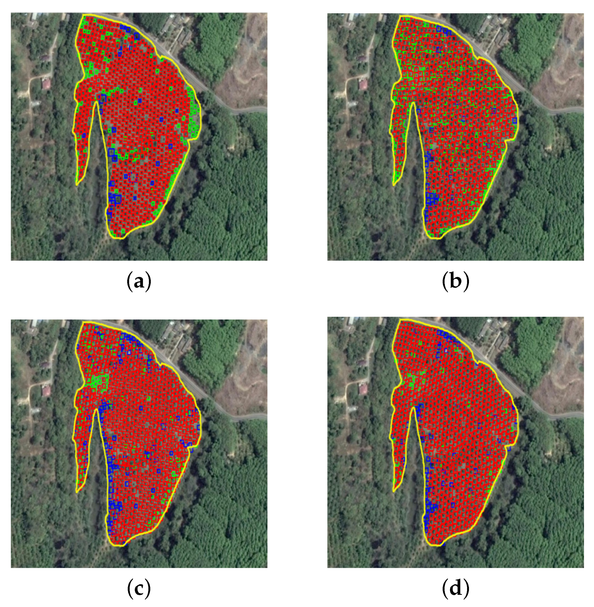
To verify the validity of this method, the four methods of region-growing [30], template-matching [11], convolutional neural network (CNN) [21], and the progressive cascaded convolutional neural network were compared in these three test areas. Figure 10, Figure 11 and Figure 12 show the tree detection results of Test Area 1, 2 and 3 using different methods, with the red rectangular bounding box indicating the trees that were successfully detected, the blue rectangular bounding box indicating the objects that were falsely recognised as trees, and the green rectangular bounding box indicating the trees that were ignored.
Test Area 1 represents a scenario with trees planted in a large area; the size of the sliding window (W) in the region-growing method was set to 5, and the pixel difference thresholds (T) between the template and the sample in the template-matching method were set to 0.36 and 0.4, respectively. The network parameters of the convolutional neural network and progressive cascaded network were completed by automatic model training extraction, which did not need to be set up artificially. As shown in Table 1, the recall of the region-growing method is very low because the trees in Test Area 1 are denser and the area contains many newly planted small saplings. Since only the maximum value is extracted in the local region-growing method, these saplings are ignored, resulting in more omission errors. In addition, the trees planted in Test Area 1 are denser, and not all the tree templates in all circumstances can be extracted, leading to more omission errors. Although the recall of the convolutional neural network is higher than that of traditional algorithms, the precision is lower than that of the progressive cascaded convolutional neural network. Taken together, compared with other algorithms, the progressive cascaded convolutional neural network proposed in this paper has more successful detection results and the fewest omission errors. Therefore, the tree detection effect in Test Area 1 is the best.
Test Area 2 is a complex greening scene in the city that has many trees, buildings, roads and rivers. The size of the sliding window (W) in the region-growing method was set to 3, and the pixel difference threshold (T) between the template and the sample in the template-matching method was set to 0.4. The network parameters of the convolutional neural network and progressive cascaded network were completed by automatic model training extraction, which did not need to be set up artificially. As shown in Figure 11 and Table 2, in general, the detection results of several methods are not particularly high. As shown in Figure 11a, this is mainly because the algorithm cannot effectively avoid the interference of complex backgrounds and chose many wrong seed points, resulting in low precision. In Figure 11b, there are many green omission error bounding boxes in the test results of the template-matching algorithm, which is mainly because of the existence of many trees of different sizes in the complex scene. Not all templates of the trees can be obtained in advance, and the template-matching algorithm can match only an area of the same size, resulting in many trees of different types and templates being labelled as omission errors; therefore, the recall of the test results of the template-matching method is low. In this paper, the anti-jamming ability of the progressive cascaded convolutional neural network is the best, which can distinguish a certain number of hard-to-classify samples and maintain high precision, recall and F1 measure simultaneously.
Test Area 3 is a normal scene in a real forest with shadows of tress and tree adhesion. The size of the sliding window (W) in the region-growing method was set to 5, and the pixel difference threshold (T) between the template and the sample in the template-matching method was set to 0.2. The network parameters of the convolutional neural network and progressive cascaded network were completed by automatic model training extraction, which did not need to be set up artificially. As shown in Figure 12 and Table 3, because of the presence of tree shadows, the shadows of trees were used as seed points, which caused low precision. With the tree adhesion, if two or more trees were too close, they would be suppressed by NMS, which led to low recall. Similarly, template matching also has low precision and recall because of matching processing affected by changes of tree shape due to tree adhesion. At the same time, all the templates cannot be obtained in advance, leading to poor precision and recall. Lower precision and recall also result in poor F1. CNN has a better precision and recall than template matching and range growing, but the progressive cascaded convolutional neural network proposed in this paper shows more successful detection results, which can maintain high precision, recall and F1 measure simultaneously
The overall test results of the three test areas are shown in Table 4. The precision and recall of the tree detection algorithm based on the progressive cascaded convolutional neural network proposed in this paper are higher, and the F1 measure reaches 81.0%. Compared with the region-growing, the template-matching and convolutional neural network algorithms, the test results of the progressive cascaded convolutional neural network are improved by 14.5%, 18.9% and 5.0%, respectively. The proposed algorithm has good robustness and portability for complex scenes while ensuring high performance in large area planting forest scenarios, has a good promotion effect on the automatic detection precision of trees and the extraction of single tree canopy information, and provides a basis for the construction of three-dimensional virtual scenarios.
4.1.2. Significant Test of Experimental Results
Because the evaluation of each method presented above did not exclude the interference of factors such as experimental error, we next made a significant analysis of the experimental results to prove that our method is statistically different from the other methods, which can prove that our method has better performance.
In our study, the samples were not independent. Thus, the statistical significance of the difference between two methods was confirmed using McNemar’s test [31]. This is a non-parametric test that is based upon 2 by 2 confusion matrices. The McNemar’s test is based upon the standardised normal test statistic:
in which indicates the frequency of sites lying in confusion matrix element i, j, the square of z follows a chi-squared distribution with one degree of freedom, and the test equation may be expressed as:
We set a p value for test, and when , the results obtained by the two methods have significant differences. When , the statistic of McNemar’s test is 5.02. The following table presents the result of the significance test between our method and other methods in the three areas.
In Test Area 1, the test result of our method with region growing and template matching are 21.13 and 8.31, as shown in Table 5. Obviously, they are greater than 5.02, thus their difference is statistically significant. However, the result of our method and CNN is 0.04. It seems that the results are not significantly different. The reason is that the tree samples are all easy-to-classify samples in Test Area 1. Most trees are distinguished in the first branch, and the first branch is a common CNN network, thus the significant differences between our method and CNN are not reflected in this case.
In Test Area 2, the test result of our method with region growing, template matching and CNN are 13.76, 9.01 and 9.50, respectively, as shown in Table 6. Obviously, they are all greater than 5.02, thus their difference is statistically significant. Because there are many samples such as roads and buildings in Test Area 2, it is helpful to show the advantage of our method to process the samples with different difficulty levels through different branches. Generally, our method has obvious significant differences with other methods.
In Test Area 3, the test result of our method with region growing and template matching are 7.12 and 9.50, respectively, as shown in Table 7. Obviously, they are greater than 5.02, thus their difference is statistically significant. However, the result of our method and CNN is 3.14, and it seems that the results are not significantly different. The reason is that the tree samples are all hard-to-classify samples in Test Area 3. Most trees are distinguished in the last branch, thus our network degenerates into a normal CNN and our method does not have significant differences with CNN.
The experimental results in the above areas show that our method has better performance than other methods under the interference of other samples (such as roads and buildings). Of course, due to the characteristics of our method, if there is a single tree type and there are only easy-to-classify samples in the test area (such as Test Area 1) or there are only hard-to-classify samples in the test area (such as Test Area 3), our method will degenerate into a normal CNN network, thus the significant differences between our method and CNN are not reflected in these test areas.
To compare the difference between CNN and our method in Test Areas 1 and 3, we calculated the kappa coefficients of the results between two methods and ground truth. The kappa coefficients [31] are used for consistency testing and can also be used to measure the classification accuracy. The kappa coefficient of CNN and ground truth in Test Area 1 is 0.88, and the kappa coefficient of Cascaded CNN and ground truth in Test Area 1 is 0.93. The kappa coefficient of CNN and ground truth in Test Area 3 is 0.48, and the kappa coefficient of Cascaded CNN and ground truth in Test Area 3 is 0.51. Therefore, the results of our method have better accuracy than CNN. Although our method has no significant difference with CNN, our method has better consistency with ground truth.
4.2. Analysis and Discussion
4.2.1. Analysis of Test Results of Progressive Branches
To evaluate the relationship between progressive classification branches and the effect on the overall network, the detection results for different classification branches are presented in this paper. Figure 13 shows the feedback of each classification branch on different samples under the window scale () in the complex scenario of Test Area 2. Figure 13a,b shows the feedback results of Branch 1 according to the output probability. Figure 13c,d shows the feedback results obtained by Branch 2 based on the output probability. Figure 13e shows the positive sample results received by Branch 3 based on the output probability. Due to the large number of negative samples in Branch 3, the feedback results of the negative sample are not shown (only the positive samples are shown). The red dotted box shows the positive samples received, and the blue dotted box shows the negative samples that are removed.
As shown in Figure 13a, Branch 1 detects 111 positive samples that are easily distinguishable from trees, and these positive samples have a more obvious outline of the shape of the trees. Figure 13b detects 146 negative samples that are easily judged as not trees, which are generally white or mostly white from a colour point of view, while the colour of the trees is basically green; moreover, the negative samples have no obvious circular tree outlines in the boundary information. Branch 1 receives these positive samples, eliminates the negative samples and feeds them back to the feature extraction module. In this way, the remaining samples progress to the second branch extraction feature, which accelerates the detection speed of the network as a whole. As shown in Figure 13c,d, Branch 2 detects 157 positive samples and 356 negative samples, in which more roads and buildings are removed as negative samples, and trees next to some roads and rivers are received as positive samples, most of which are close to the turf vegetation on the surface, making detection more difficult. Similarly, Branch 2 is fed back to the feature extraction module, the remaining samples progress to Branch 3 for feature extraction and category judgement, and 225 positive sample trees are eventually detected. Our progressive cascaded convolutional neural network has a good ability to detect samples of different difficulty levels.
As shown in Figure 14, the network model first extracts features through the conv1 layer and pool1 layer, then enters Branch 1 and passes the full-connect layer, dropout layer, and softmax layer. The results are the feedback from Branch 1 to the feature map after the pool1 layer, and the filtered feature maps continue to extract deeper features through the conv2 layer and pool2 layer. Similarly, through Branch 2, the results are fed back to the feature map after the pool2 layer, and the filtered feature maps enter Branch 3. The network model can filter the easy-to-classify samples in the shallow branch to speed up the detection speed, while the deep branch can better extract and identify the hard-to-classify samples.
We also analysed the results of each branch in Test Area 3, as shown in Figure 15. Almost no positive samples are received in Branch 1, and it is likely that the feature is not extracted enough in the network to distinguish positive samples under the threshold. Many tree shadows can be identified; this should be because the shadow of the tree is sufficiently obvious as a negative sample to be recognised based on underlying features. The results of Branch 2 are similar to those of Branch 1. However, because of the increasing number of network layers, more features are extracted, thus the positive and negative samples received and removed by Branch 2 are more than those by Branch 1. Most trees are detected in the last branch because there are tree adhesion and shadow of trees in this area, which causes most trees to differ from the training samples so that they cannot reach the threshold of the first two branches, and it is necessary to extract deeper features to determine if they are trees. Thus, they are hard-to-classify samples. This may cause a problem. When there are all hard-to-classify samples in our detection area, the first two branches would not work. In this case, our network may degenerate into a normal CNN network. Thus, this is a problem that we need to explore and solve in the future.
4.2.2. Influence of Different Sliding Window Scales on Test Results
The size of trees varies in complex scenarios, for example, in Test Area 1, the radius of trees ranges from 2.5 m to 5 m. To compare the detection performance of different algorithms for trees of different sizes, the scale of the sliding window can be used to substitute for the tree size. Sliding window sizes from to were evaluated, and the test results for six scales are shown in Figure 16, Figure 17 and Figure 18.
The comparison of precision, recall and F1 measure values of the region-growing, template-matching, convolutional neural network and progressive cascaded convolutional neural network methods for the detection of trees of different sizes in complex scenarios showed they can be varied. When the trees are small, the detection performance of the progressive cascaded convolutional neural network in this paper is greatly improved compared with the region-growing and template-matching methods but is lower than that of the convolutional neural network algorithm. As the size of trees to be detected increases, the precision of the region-growing method decreases gradually while the recall increases gradually, and the F1 measure is not high overall. This is mainly because the region-growing method can only extract the maximum value of the local area, resulting in small trees that may be ignored because their maximum value cannot be detected. The template matching method has a high precision for tree detection in different shapes and sizes, but the recall is very low, and the F1 measure is not high overall. The main reason is that the template-matching method needs to calculate the error of each pixel value in each window, thus the matching is more accurate, and, because of the diversity of trees, sufficient tree templates cannot be collected for features, thus the recall is not ideal. All the precision, recall, and F1 measures of the convolutional neural network show a downward trend. The progressive cascaded network begins to highlight an obvious advantage and exceeds the convolutional neural network in precision, recall and F1 measure. In addition, our method is relatively stable compared with the other three algorithms. At the same time, when the trees are small or large, the progressive cascaded convolutional neural network and convolutional neural network are lower in precision, recall and F1 measure than when the trees are of normal scale. The reason is that when these trees need to be detected using very small or large sliding window, the strategy taken is to transform the window into the same scale (the scale of the training sample), whether it is scale expansion or scale reduction, compared with the original window scale, thus information will be lost, resulting in the precision of the tree detection algorithm not being very ideal. In general, the progressive cascaded convolutional neural network proposed in this paper has fewer errors of commission and omission in complex scenes with more background interference and diverse tree morphology and has more ideal detection results than other algorithms.
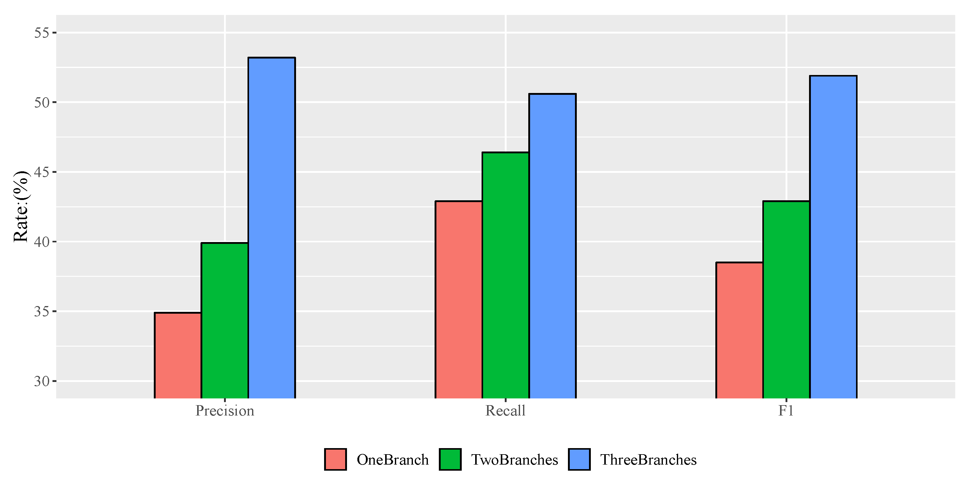
4.2.3. Influence of Different Numbers of Branches on the Detection Performance of Cascaded Models
To evaluate the effect of convolutional neural networks with different numbers of branches on the detection performance of the model after cascading, the results of the detection precision, recall and F1 measure of the cascaded convolutional neural networks with one branch, two branches, and three branches in Test Area 1, 2 and 3 were compared, as shown in Figure 19, Figure 20 and Figure 21.
As shown in Figure 19, Figure 20 and Figure 21, the precision, recall and F1 measure of the three branch networks proposed in this paper are the highest in the three test areas. Adding multiple branches can be used to detect samples of different difficulties, thus the performance of the detection can be improved gradually.
5. Conclusions
High-resolution remote sensing images have been widely used in urban greening planning, forest management, large area forest yield estimation and other applications. Currently, researchers have developed a variety of methods to extract single trees and their features from various types of digital aerial photographs. However, the generalisation performance of the existing single-tree detection methods is weak; it is difficult to detect the scene of a complex forest because of the similar colour between the tree and background, unclear canopy contour and abnormal shape caused by illumination shadows. Therefore, these existing methods cannot be used in a wide range of tree detection scenarios.
To detect single trees automatically and effectively, a single tree detection method with a high-resolution remote sensing image based on a progressive cascaded convolutional neural network is proposed in this paper. Most existing studies are based on expensive and hard-to-obtain satellite remote sensing images, and, in this study, different types of single tree samples from high-resolution images in Google Maps were calibrated and used to train cascaded convolutional neural networks. The progressive cascading of three convolutional neural networks was carried out, allowing different classification branches of the network to train samples of different difficulties. Simultaneously, a two-phase training method was adopted to speed up the training process. After model training, this model was used to detect single trees in three test areas. The test results show that the single tree detection method with a high-resolution image based on the cascaded convolutional neural network proposed in this paper is more effective than the existing methods. It is believed that the algorithm will have a wider application scenario in the future of diverse tree detection scenarios.
However, the problems encountered in the actual detection process are much more than these. For example, there are cases where adjacent trees are stuck in many scenarios. Creating effective distinguishing statistics on these trees has become an urgent problem to be solved in future work. At the same time, the single tree detection method based on sliding windows needs to scale the target window of different sizes, which will cause the problem of loss of target information and is a major cause of errors of commission and omission. For targets of different scales, even a small number of targets requires a sliding calculation of the entire image, resulting in extremely low efficiency, which will also be the focus of future work.
Author Contributions
Conceptualization, T.D.; Methodology, Y.S. and J.Z.; Original draft preparation, J.Z.; Paper writing Y.S.; Data quality check, T.D.; Data validation, Y.Y.; Paper revision, T.D., Y.S. and Y.Y.; Writing-revision & editing, T.D. and J.F.; Project Administration, J.F.
Funding
This work was supported by the following foundations: the National Natural Science Foundation of China (No.61572437, No.61672464), and the Key Research and Development Project of Zhejiang Province (No.2017C01013).
Conflicts of Interest
The authors declare no conflict of interest.
References
- Congalton, R.G.; Gu, J.; Yadav, K.; Thenkabail, P.; Ozdogan, M. Global Land Cover Mapping: A Review and Uncertainty Analysis. Remote Sens. 2014, 6, 12070–12093. [Google Scholar] [CrossRef] [Green Version]
- Treitz, P.; Rogan, J. Remote sensing for mapping and monitoring land-cover and land-use change—An introduction. Prog. Plan. 2004, 61, 269–279. [Google Scholar] [CrossRef]
- Walsworth, N.; King, D. Image modelling of forest changes associated with acid mine drainage. Aspen Bibliogr. 1999, 25, 567–580. [Google Scholar] [CrossRef]
- Erikson, M. Two Preprocessing Techniques Based on Grey Level and Geometric Thickness to Improve Segmentation Results. Pattern Recogn. Lett. 2006, 27, 160–166. [Google Scholar] [CrossRef]
- Novotnỳ, J.; Hanuš, J.; Lukeš, P.; Kaplan, V. Individual tree crowns delineation using local maxima approach and seeded region growing technique. In Proceedings of the Symposium GIS Ostrava, Ostrava, Czech Republic, 23–26 January 2011; pp. 27–39. [Google Scholar]
- Culvenor, D.S. TIDA: An algorithm for the delineation of tree crowns in high spatial resolution remotely sensed imagery. Comput. Geosci. 2002, 28, 33–44. [Google Scholar] [CrossRef]
- Hirschmugl, M.; Ofner, M.; Raggam, J.; Schardt, M. Single tree detection in very high resolution remote sensing data. Remote Sens. Environ. 2007, 110, 533–544. [Google Scholar] [CrossRef]
- Pouliot, D.; King, D.; Bell, F.; Pitt, D. Automated tree crown detection and delineation in high-resolution digital camera imagery of coniferous forest regeneration. Remote Sens. Environ. 2002, 82, 322–334. [Google Scholar] [CrossRef]
- Pollock, R. The Automatic Recognition of Individual Trees in Aerial Images of Forests Based on a Synthetic Tree Crown Image Model. Ph.D. Thesis, University of British Columbia, Vancouver, BC, Canada, 1996. [Google Scholar]
- Larsen, M.; Rudemo, M. Optimizing templates for finding trees in aerial photographs. Pattern Recognit. Lett. 1998, 19, 1153–1162. [Google Scholar] [CrossRef]
- Tarp-Johansen, M.J. Automatic stem mapping in three dimensions by template matching from aerial photographs. Scand. J. For. Res. 2002, 17, 359–368. [Google Scholar] [CrossRef]
- Hellesen, T.; Matikainen, L. An object-based approach for mapping shrub and tree cover on grassland habitats by use of LiDAR and CIR orthoimages. Remote Sens. 2013, 5, 558–583. [Google Scholar] [CrossRef]
- Laliberte, A.S.; Rango, A.; Havstad, K.M.; Paris, J.F.; Beck, R.F.; McNeely, R.; Gonzalez, A.L. Object-oriented image analysis for mapping shrub encroachment from 1937 to 2003 in southern New Mexico. Remote Sens. Environ. 2004, 93, 198–210. [Google Scholar] [CrossRef]
- Malek, S.; Bazi, Y.; Alajlan, N.; AlHichri, H.; Melgani, F. Efficient framework for palm tree detection in UAV images. IEEE J. Sel. Top. Appl. Earth Obs. Remote Sens. 2014, 7, 4692–4703. [Google Scholar] [CrossRef]
- Yang, L.; Wu, X.; Praun, E.; Ma, X. Tree detection from aerial imagery. In Proceedings of the 17th ACM SIGSPATIAL International Conference on Advances in Geographic Information Systems, Seattle, WA, USA, 4–6 November 2009; ACM: New York, NY, USA, 2009; pp. 131–137. [Google Scholar] [Green Version]
- Krizhevsky, A.; Sutskever, I.; Hinton, G.E. Imagenet classification with deep convolutional neural networks. In Proceedings of the Advances in Neural Information Processing Systems, Lake Tahoe, NV, USA, 3–6 December 2012; pp. 1097–1105. [Google Scholar]
- Le, Q.V. Building high-level features using large scale unsupervised learning. In Proceedings of the 2013 IEEE International Conference on Acoustics, Speech and Signal Processing (ICASSP 2013), Vancouver, BC, Canada, 26–31 May 2013; pp. 8595–8598. [Google Scholar]
- Hinton, G.; Deng, L.; Yu, D.; Dahl, G.E.; Mohamed, A.R.; Jaitly, N.; Senior, A.; Vanhoucke, V.; Nguyen, P.; Sainath, T.N.; et al. Deep neural networks for acoustic modeling in speech recognition: The shared views of four research groups. IEEE Signal Process. Mag. 2012, 29, 82–97. [Google Scholar] [CrossRef]
- Sainath, T.N.; Mohamed, A.R.; Kingsbury, B.; Ramabhadran, B. Deep convolutional neural networks for LVCSR. In Proceedings of the 2013 IEEE International Conference on Acoustics, Speech and Signal Processing (ICASSP 2013), Vancouver, BC, Canada, 26–31 May 2013; pp. 8614–8618. [Google Scholar]
- Zhu, X.X.; Tuia, D.; Mou, L.; Xia, G.S.; Zhang, L.; Xu, F.; Fraundorfer, F. Deep learning in remote sensing: A comprehensive review and list of resources. IEEE Geosci. Remote Sens. Mag. 2017, 5, 8–36. [Google Scholar] [CrossRef]
- Li, W.; Fu, H.; Yu, L.; Cracknell, A. Deep learning based oil palm tree detection and counting for high-resolution remote sensing images. Remote Sens. 2016, 9, 22. [Google Scholar] [CrossRef]
- Guirado, E.; Tabik, S.; Alcaraz-Segura, D.; Cabello, J.; Herrera, F. Deep-learning versus OBIA for scattered shrub detection with Google earth imagery: Ziziphus Lotus as case study. Remote Sens. 2017, 9, 1220. [Google Scholar] [CrossRef]
- Ren, S.; He, K.; Girshick, R.; Sun, J. Faster r-cnn: Towards real-time object detection with region proposal networks. In Proceedings of the Advances in Neural Information Processing Systems, Montreal, QC, Canada, 7–12 December 2015; pp. 91–99. [Google Scholar]
- Redmon, J.; Divvala, S.; Girshick, R.; Farhadi, A. You only look once: Unified, real-time object detection. In Proceedings of the IEEE Conference on Computer Vision and Pattern Recognition, Las Vegas, NV, USA, 26 June–1 July 2016; pp. 779–788. [Google Scholar]
- Angelova, A.; Krizhevsky, A.; Vanhoucke, V.; Ogale, A.S.; Ferguson, D. Real-Time Pedestrian Detection with Deep Network Cascades. In Proceedings of the 26th British Machine Vision Conference (BMVC ’15), Swansea, UK, 7–10 September 2015. [Google Scholar]
- Lu, K.; Chen, J.; Little, J.J.; He, H. Light cascaded convolutional neural networks for accurate player detection. In Proceedings of the 28th British Machine Vision Conference (BMVC ’17), London, UK, 4–7 September 2017. [Google Scholar]
- Abadi, M.; Barham, P.; Chen, J.; Chen, Z.; Davis, A.; Dean, J.; Devin, M.; Ghemawat, S.; Irving, G.; Isard, M.; et al. Tensorflow: A system for large-scale machine learning. In Proceedings of the 12th USENIX Symposium on Operating Systems Design and Implementation (OSDI ’16), Savannah, GA, USA, 2–4 November 2016; Volume 16, pp. 265–283. [Google Scholar]
- Tabik, S.; Peralta, D.; Herrera-Poyatos, A.; Herrera, F. A snapshot of image pre-processing for convolutional neural networks: case study of MNIST. Int. J. Comput. Intell. Syst. 2017, 10, 555–568. [Google Scholar] [CrossRef] [Green Version]
- Peralta, D.; Triguero, I.; García, S.; Saeys, Y.; Benitez, J.M.; Herrera, F. On the use of convolutional neural networks for robust classification of multiple fingerprint captures. Int. J. Intell. Syst. 2018, 33, 213–230. [Google Scholar] [CrossRef]
- Zhen, Z.; Quackenbush, L.J.; Stehman, S.V.; Zhang, L. Agent-based region growing for individual tree crown delineation from airborne laser scanning (ALS) data. Int. J. Remote Sens. 2015, 36, 1965–1993. [Google Scholar] [CrossRef]
- Foody, G.M. Thematic Map Comparison: Evaluating the Statistical Significance of Differences in Classification Accuracy. Photogramm. Eng. Remote Sens. 2004, 70, 627–633. [Google Scholar] [CrossRef]
Figure 1.
Schematic diagram of test areas.

Figure 2.
Flowchart of tree detection.

Figure 3.
The composition of samples.

Figure 4.
The diagram of classification branch.

Figure 5.
Progressive cascaded convolutional neural network.

Figure 6.
Examples of hard-to-classify samples.

Figure 7.
Sharing mechanism of feature map.

Figure 8.
Sliding window for label prediction.

Figure 9.
The process of non-maximum suppression (NMS).

Figure 10.
Results of different methods in Test Area 1: (a) Region-growing; (b) Template-matching; (c) Convolutional neural network; and (d) Progressive cascaded convolutional neural network.
Figure 10.
Results of different methods in Test Area 1: (a) Region-growing; (b) Template-matching; (c) Convolutional neural network; and (d) Progressive cascaded convolutional neural network.

Figure 11.
Results of different methods in Test Area 2: (a) Region-growing; (b) Template-matching; (c) Convolutional neural network; and (d) Progressive cascaded convolutional neural network.
Figure 11.
Results of different methods in Test Area 2: (a) Region-growing; (b) Template-matching; (c) Convolutional neural network; and (d) Progressive cascaded convolutional neural network.

Figure 12.
Results of different methods in Test Area 3: (a) Region-growing; (b) Template-matching; (c) Convolutional neural network; and (d) Progressive cascaded convolutional neural network.
Figure 12.
Results of different methods in Test Area 3: (a) Region-growing; (b) Template-matching; (c) Convolutional neural network; and (d) Progressive cascaded convolutional neural network.

Figure 13.
Results for different classification branches in Test Area 2 (window size ): (a) Positive samples received in Branch 1; (b) Negative samples removed in Branch 1; (c) Positive samples received in Branch 2; (d) Negative samples removed in Branch 2; and (e) Positive samples received in Branch 3.

Figure 14.
The progressive process of classification branches.

Figure 15.
Results for different classification branches in Test Area 3 (window size ): (a) Positive samples received in Branch 1; (b) Negative samples removed in Branch 1; (c) Positive samples received in Branch 2; (d) Negative samples removed in Branch 2; and (e) Positive samples received in Branch 3.

Figure 16.
Comparison of detection precision for different methods.

Figure 17.
Comparison of detection recall for different methods.

Figure 18.
Comparison of F1 measurements for different methods.

Figure 19.
Comparison of detection results for different numbers of branch in Test Area 1.

Figure 20.
Comparison of detection results for different numbers of branch in Test Area 2.

Figure 21.
Comparison of detection results for different numbers of branch in Test Area 3.


Table 1.
The comparisons of Test Area 1.
| Detection Model | TP | FP | FN | Precision | Recall | F1 |
|---|---|---|---|---|---|---|
| Region-growing | 677 | 36 | 131 | 95.0% | 83.8% | 89.0% |
| Template-matching | 563 | 28 | 245 | 95.3% | 69.7% | 80.5% |
| CNN | 729 | 107 | 79 | 87.2% | 90.2% | 88.7% |
| Cascaded CNN | 766 | 64 | 42 | 92.3% | 94.8% | 93.5% |
Table 2.
The comparisons of Test Area 2.
| Detection Model | TP | FP | FN | Precision | Recall | F1 |
|---|---|---|---|---|---|---|
| Region-growing | 114 | 191 | 140 | 37.4% | 44.9% | 40.8% |
| Template-matching | 71 | 25 | 183 | 74.0% | 28.0% | 40.6% |
| CNN | 164 | 133 | 90 | 55.2% | 64.6% | 59.5% |
| Cascaded CNN | 186 | 88 | 68 | 67.9% | 73.2% | 70.5% |
Table 3.
The comparisons of Test Area 3.
| Detection Model | TP | FP | FN | Precision | Recall | F1 |
|---|---|---|---|---|---|---|
| Region-growing | 109 | 270 | 152 | 28.8% | 41.8% | 34.1% |
| Template-matching | 52 | 148 | 209 | 26.0% | 19.9% | 22.6% |
| CNN | 98 | 49 | 163 | 66.7% | 37.5% | 48.0% |
| Cascaded CNN | 132 | 116 | 129 | 53.2% | 50.6% | 51.9% |
Table 4.
The comparisons of the all areas.
| Detection Model | TP | FP | FN | Precision | Recall | F1 |
|---|---|---|---|---|---|---|
| Region-growing | 900 | 497 | 411 | 64.4% | 68.6% | 66.5% |
| Template-matching | 686 | 201 | 637 | 77.3% | 51.9% | 62.1% |
| CNN | 1055 | 398 | 268 | 72.6% | 79.7% | 76.0% |
| Cascaded CNN | 1084 | 268 | 239 | 80.2% | 81.9% | 81.0% |
Table 5.
The results of McNemar’s test in Test Area 1.
| ID | Methods | Cascaded CNN | McNemar’s Test | |||
|---|---|---|---|---|---|---|
| Correct | Incorrect | ∑ | ||||
| 1 | Region-growing | Correct | 653 | 24 | 677 | 21.13 |
| Incorrect | 113 | 18 | 131 | |||
| ∑ | 766 | 42 | 808 | |||
| 2 | Template-matching | Correct | 532 | 31 | 563 | 8.31 |
| Incorrect | 234 | 11 | 245 | |||
| ∑ | 766 | 42 | 808 | |||
| 3 | CNN | Correct | 691 | 38 | 729 | 0.04 |
| Incorrect | 75 | 4 | 79 | |||
| ∑ | 766 | 42 | 808 | |||
Table 6.
The results of McNemar’s test in Test Area 2.
| ID | Methods | Cascaded CNN | McNemar’s Test | |||
|---|---|---|---|---|---|---|
| Correct | Incorrect | ∑ | ||||
| 1 | Region-growing | Correct | 97 | 17 | 114 | 13.76 |
| Incorrect | 89 | 51 | 140 | |||
| ∑ | 186 | 68 | 254 | |||
| 2 | Template-matching | Correct | 62 | 9 | 71 | 9.01 |
| Incorrect | 124 | 59 | 183 | |||
| ∑ | 186 | 68 | 254 | |||
| 3 | CNN | Correct | 131 | 33 | 164 | 9.50 |
| Incorrect | 55 | 35 | 90 | |||
| ∑ | 186 | 68 | 254 | |||
Table 7.
The results of McNemar’s test in Test Area 3.
| ID | Methods | Cascaded CNN | McNemar’s Test | |||
|---|---|---|---|---|---|---|
| Correct | Incorrect | ∑ | ||||
| 1 | Region-growing | Correct | 44 | 65 | 109 | 7.12 |
| Incorrect | 88 | 64 | 152 | |||
| ∑ | 132 | 129 | 261 | |||
| 2 | Template-matching | Correct | 14 | 38 | 52 | 9.50 |
| Incorrect | 118 | 91 | 209 | |||
| ∑ | 132 | 129 | 261 | |||
| 3 | CNN | Correct | 57 | 41 | 98 | 3.14 |
| Incorrect | 75 | 88 | 163 | |||
| ∑ | 132 | 123 | 261 | |||
© 2019 by the authors. Licensee MDPI, Basel, Switzerland. This article is an open access article distributed under the terms and conditions of the Creative Commons Attribution (CC BY) license (http://creativecommons.org/licenses/by/4.0/).
Share and Cite
MDPI and ACS Style
Dong, T.; Shen, Y.; Zhang, J.; Ye, Y.; Fan, J. Progressive Cascaded Convolutional Neural Networks for Single Tree Detection with Google Earth Imagery. Remote Sens. 2019, 11, 1786. https://doi.org/10.3390/rs11151786
AMA Style
Dong T, Shen Y, Zhang J, Ye Y, Fan J. Progressive Cascaded Convolutional Neural Networks for Single Tree Detection with Google Earth Imagery. Remote Sensing. 2019; 11(15):1786. https://doi.org/10.3390/rs11151786
Chicago/Turabian StyleDong, Tianyang, Yuqi Shen, Jian Zhang, Yang Ye, and Jing Fan. 2019. "Progressive Cascaded Convolutional Neural Networks for Single Tree Detection with Google Earth Imagery" Remote Sensing 11, no. 15: 1786. https://doi.org/10.3390/rs11151786
Note that from the first issue of 2016, this journal uses article numbers instead of page numbers. See further details here.