A Density-Based Approach for Leaf Area Index Assessment in a Complex Forest Environment Using a Terrestrial Laser Scanner

Abstract

Forests are an important part natural ecosystems, by for example providing food, fiber, habitat, and biodiversity, all of which contribute to stable natural systems. Assessing and modeling the structure and characteristics of forests, e.g., Leaf Area Index (LAI), volume, biomass, etc., can lead to a better understanding and management of these resources. In recent years, Terrestrial Laser Scanning (TLS) has been recognized as a tool that addresses many of the limitations of manual and traditional forest data collection methods. In this study, we propose a density-based approach for estimating the LAI in a structurally-complex forest environment, which contains variable and diverse structural attributes, e.g., non-circular stem forms, dense canopy and below-canopy vegetation cover, and a diverse species composition. In addition, 242 TLS scans were collected using a portable low-cost scanner, the Compact Biomass Lidar (CBL), in the Hawaii Volcanoes National Park (HAVO), Hawaii Island, USA. LAI also was measured for 242 plots in the site, using an AccuPAR LP-80 ceptometer. The first step after cleaning the point cloud involved detecting the higher forest canopy in the light detection and ranging (lidar) point clouds, using normal change rate assessment. We then estimated Leaf Area Density (LAD), using a voxel-based approach, and divided the canopy point cloud into five layers in the Z (vertical) direction. These five layers subsequently were divided into voxels in the X direction, where the size of these voxels were obtained based on inter-quartile analysis and the number of points in each voxel. We hypothesized that the intensity returned to the lidar system from woody materials, like branches, would be higher than from leaves, due to the liquid water absorption feature of the leaves and higher reflectance for woody material at the 905 nm laser wavelength. We also differentiated between foliar and woody materials using edge detection in the images from projected point clouds and evaluated the density of these regions to support our hypothesis. Density of points, or the number of points divided by the volume of a grid, in a 3D grid size of 0.1 m, was calculated for each of the voxels. The grid size was determined by investigating the size of the branches in the lower portion of the canopy. Subsequently, we fitted a Kernel Density Estimator (KDE) to these values, with the threshold set based on half of the area under the curve in each of the density distributions. All the grids with a density below the threshold were labeled as leaves, while those grids above the threshold were identified as non-leaves. Finally, we modeled LAI using the point densities derived from the TLS point clouds and the listed analysis steps. This model resulted in an $R^2$ value of 0.88. We also estimated the LAI directly from lidar data using the point densities and calculating LAD, which is defined as the total one-sided leaf area per unit volume. LAI can be obtained as the sum of the LAD values in all the voxels. The accuracy of LAI estimation was 90%, with an RMSE value of 0.31, and an average overestimation of $9\%$ in TLS-derived LAI, when compared to field-measured LAI. Algorithm performance mainly was affected by the vegetation density and complexity of the canopy structures. It is worth noting that, since the LAI values cannot be considered spatially independent throughout all the plots in this site, we performed semivariogram analysis on the field-measured LAI data. This analysis showed that the LAI values can be assumed to be independent in plots that are at least 30 m apart. As a result, we divided the data into six subsets in which the plots were 30 m spaced. The $R^2$ values for these subsets, based on modeling of the field-measured LAI using leaf point density values, ranged between 0.84–0.96. The results bode well for using this method for efficient, automatic, and accurate/precise estimation of LAI values in complex forest environments, using a low-cost, rapid-scan TLS.

1. Introduction

The spatial distribution of foliage in a forest canopy controls energy transfer to the lower plant components and also the ground [1], the interception of precipitation [2], photosynthesis [3], and other phenomena. As a result, leaf properties and canopy structure are important inputs in eco-physical models of forest environments [4]. Leaf Area Index (LAI) is an indicator for predicting photosynthetic primary production, evapotranspiration and crop growth [5]. LAI typically is defined as the vertically integrated one-sided area of leaves per unit ground surface area on a horizontal plane [6], and traditionally is measured through destructive sampling. Since LAI cannot be easily measured through non-destructive methods, effective LAI (LAIe) is more commonly measured in the field and calibrated to true LAI [6]. The difference between LAI and LAIe is that effective LAI does not differentiate between branches and foliar components. LAI effectively has been linked to vertical laser pulse return profiles using light detection and ranging (lidar). One elegant method is to calculate the ratio of the number of returns below the canopy to the total number of returns, and assume that this is related to gap fraction (P) of the canopy [7]:

$$P\approx N_{bc}/N_{total},$$

(1)

where $N_{total}$ is the total number of returns and $N_{bc}$ is the number of returns below some height above the ground surface (usually between 1 and 3 m). It has also been shown that this formula does not always provide a direct estimate of the gap fraction, but the ratio shown in Formula (2) can be used for LAI estimation when using airborne lidar data [7]:

$$LAI=-ln\left(P\right)/k,$$

(2)

where k is the extinction coefficient. An assumption of random or spherical leaf distribution is typically used, which results in the k value of 0.5 [8]. In reality, k values range from 0.25–0.75 [9].

An alternative voxel-based approach for gap fraction estimation was presented in [10]. The authors sampled a plot with an area of 20 m by 40 m with fifteen Terrestrial Laser Scanning (TLS) scans. These scans were then co-registered, providing a dense point cloud. The point cloud was partitioned into different voxels and the number of points were counted in each voxel. The authors estimated Plant Area Index (PAI) for two different point clouds, namely leaf-on and leaf-off. PAI was calculated using the following equation:

$$PA{I}_i=-ln(\frac{N_i}{N_i+I_i}),$$

(3)

where $N_i$ is the number of laser beams passing through voxel number i, and $I_i$ is the number of returns within the voxel i. The plot level PAI was then obtained by taking the average of all the voxel PAI values. LAI was estimated as the difference between the PAI measurements for leaf-on and leaf-off point clouds. The resulting LAIs were in the range of 1.4–1.8, which is significantly lower than the LAI values obtained via traditional manual methods (LAI = 2.7–8.2).

Another approach to assessing LAI using TLS is by estimating Leaf Area Density (LAD) [11]. LAD can be described as the total one-sided leaf area per unit volume [12] and the integration of a LAD profile vertically yields the LAI [13]. LAD can be estimated using direct, semi-direct, or indirect methods on-site [14]. The direct approach includes manual counting and measuring of leaves, while semi-direct methods count the contact of a leaf with probes inserted into the canopy [15]. Indirect techniques involve the application of passive optical devices, based on a gap fraction method [15]. However, the mentioned methods are limited in accuracy and in the spatial explicitness of their estimates [14]. As a result, the extracted 3D structures from lidar data can be used for measuring LAD [11]. One such manual method for finding the contact frequencies in the canopy is presented in [15], which is known as the inclined point quadrat method. In this method, a probe is pierced into the canopy at known heights and angles, and then the number of contact points with the foliage components are tallied. This method estimates the probability that a laser pulse penetrating the canopy will contact a foliage component. In Equation (4), N denotes the contact frequency, ${\theta }_v$ and ${\varphi }_v$ represent elevation and azimuth angle respectively, and H is the height. G is the projection function denoting the unit mean projected foliage area, and $l\left(h\right)$ is the height-dependent LAD:

$$N(H,{\theta }_v,{\varphi }_v)={\int }_0^{H}G(h,{\theta }_v,{\varphi }_v)(l\left(h\right)/\cos {\theta }_v)dh.$$

(4)

For simplifying this equation, typically one assumes that the LAD and projection function are independent of height. Thus, we can have:

$$N(L,{\theta }_v,{\varphi }_v)=G({\theta }_v,{\varphi }_v)(LAD/cos{\theta }_v),$$

(5)

where $LAD$ is the height-independent LAD. A challenge of this method is that it is difficult to measure this quantity [12]. One more convenient approach can be describing the gap fraction based on the same terms, with the assumption of a random spatial distribution for small leaves:

$$P_0\left({\theta }_v\right)=exp(-N({\theta }_v,{\varphi }_v)=exp(-G({\theta }_v,{\varphi }_v)LAD/\cos {\theta }_v).$$

(6)

In later efforts, [16] included the clumping effect and with the assumption of azimuthal symmetry, provided Equation (7) for gap fraction:

$$P_0\left({\theta }_v\right)=exp(-G\left({\theta }_v\right)\Omega LAD/\cos {\theta }_v),$$

(7)

where $\Omega$ describes the clumping index and $\Omega LAD$ provides the effective LAI (${LAI}_e$).

The mentioned projection function depends on the leaf normal orientation distribution. However, by restricting the penetration zenith angles to 57.5${}^{°}$, the computation of the leaf normal orientation distribution can be neglected [15]). These authors have shown that $G\left({\theta }_v\right)$ at the angle of 57.5${}^{°}$ equals 0.5. Effective LAI then can be described with this model:

$$LA{I}_e=1.1N\left({57.5}^{°}\right),$$

(8)

where $LA{I}_e$ is effective LAI and N(57.5${}^{°}$) denotes the number of contact points with vegetation at a zenith angle of 57.5${}^{°}$.

TLS, on the other hand, provides a fine spatial or angular resolution, thereby allowing the internal regions of the canopy to be evaluated from a ground perspective, making LAD estimation more accurate [17]. One of the important considerations of LAD estimation is the ability to describe the spatial distribution of leaves, separate from the woody canopy structures [14]. LAD estimation is highly affected by whether the leafy and woody parts are separated in the point cloud, and many studies have used manual techniques for leaf classification (e.g., [17]), although these approaches are time consuming. However, the intensity of the reflected pulse often can be used to distinguish a leaf from woody structures in the canopy [14], even though the intensity is affected by the range and incidence angle. Geometric methods have also been used for separating leaves and branches in TLS data [18], but obtaining geometric attributes of leaves and canopy-level structures is challenging, and is impacted by the angular scan resolution of the system, the pulse frequency, etc. [19]. We therefore opted for a density-based approach for segmenting the leaves in TLS point clouds, since such a method is more robust against variable system characteristics and can be applied more routinely; this approach will be described in detail in the Methods section.

As mentioned earlier, LAI is calculated by the sum of the LAD measurements in vertical layers of the forest canopy:

$$LAI={\int }_0^{h}LAD\left(z\right)dz.$$

(9)

In a more recent study, Shihua et al. [11] used a voxel-based method for estimating the LAD of an individual tree using point cloud segmentation of TLS data. They differentiated between the leafy and woody materials using the normal differences of the two. They also partitioned point cloud into sub-regions to improve the accuracy of the leaf extraction. It is important to note in this context that such point cloud segmentation approaches can be classified into three main categories, namely edge-detection, region-growth (blob-growth), and hybrid methods.

Edge-detection techniques find the breaks in the surface of the point cloud, whereas the region-growth methods detect the continuous surfaces that are similar in geometric properties, and the hybrid methods combine the two mentioned approaches [20]. Normals of the point cloud can be used in segmentation of unorganized 3D point clouds. In short, the more the surface structure changes in adjacent areas, the more the normals of these areas are oriented differently. Figure 1 shows an illustration of the difference in normal distributions in leaves and branches.

The normal differences of the leaf point cloud is generally smaller than those from non-leaf materials [11], and for a point, p, in the point cloud, it is measured by the following equation:

$$\Delta n(p,r)=(1/N)\sum _{i=1}^N(n\left(p\right)-n\left(p_i\right)),$$

(10)

where $n\left(p\right)$ is the normal of the point cloud in point p, and r is the average spatial distance between the two leaves [11]. The leaf point cloud is extracted using the magnitude of $\Delta n$ and compared to a threshold. One common way for finding the threshold is using the Otsu algorithm [21].

Furthermore, for this voxel-based method of LAD assessment, the point cloud is segmented into layers in the X direction, and LAD is calculated in all those layers using a voxel-based canopy profiling (VCP) method [17]. LAD between heights h and $h+\Delta h$ is calculated using the following equation:

$$LAD(h,\Delta h)=\alpha \left(\theta \right)(1/\Delta h)\sum _{k=m_h}^{m_{h+\Delta h}}\frac{n_1\left(k\right)}{n_1\left(k\right)+n_p\left(k\right)},$$

(11)

where $\theta$ is the zenith angle of the lidar beam, $\Delta h$ is the layer thickness, $m_h$ and $m_{h+\Delta h}$ denote the voxel coordinates on the vertical axis, corresponding to heights h and $h+\Delta h$, and $n_1\left(k\right)$ and $n_p\left(k\right)$ indicate the number of voxels containing leaf points and excluding, respectively. Thereby, $n_1\left(k\right)+n_p\left(k\right)$ gives the total number of incident laser beams in the k-th layer. $\alpha \left(\theta \right)$ is defined as:

$$\alpha \left(\theta \right)=\cos \theta /G\left(\theta \right).$$

(12)

$\alpha \left(\theta \right)$ is a correction factor of the leaf inclination angle at the laser zenith angle of $\theta$. $G\left(\theta \right)$ is the mean projection of a unit leaf area on a plane perpendicular to the direction of the laser beam. A symmetrical shape for the leaves is assumed for measuring of $G\left(\theta \right)$. It is defined as:

$$G\left(\theta \right)=(1/2\pi ){\int }_0^{2\pi }{\int }_0^{\pi /2}g\left({\theta }_L\right)\left|\cos (n_B,n_L)\right|d{\theta }_{L}d{\varphi }_L,$$

(13)

where ${\theta }_L$ indicates the leaf inclination angle, ${\varphi }_L$ is the azimuth angle of the normal, and $n_B$ and $n_L$ are obtained using the following equations:

$$n_B=(\sin \theta \cos \theta \cos \varphi ,\sin \theta \sin \varphi ,\cos \theta ),$$

(14)

$$n_L=(\sin {\theta }_L\cos {\theta }_L,\sin {\theta }_L\sin {\varphi }_L,\cos {\theta }_L).$$

(15)

$n_B$ and $n_L$ are unit vectors showing the direction of the lidar beam and the direction of the leaf normal, respectively.

The TLS used in this study provides lower-density data, due to lower angular resolution and pulse frequency, compared to commercial higher-cost systems. The minimum angular step-width of CBL is 4.36 mrad, which result in lidar point clouds with lower associated point density when compared to higher cost systems, for which the minimum angular step-width can be as small as 0.02 mrad [22]. These low-density data introduce challenges to automatic leaf segmentation algorithms. We therefore evaluated the ability of this arguably more operational system (low-cost; rapid-scan) to automatically extract leaf points, and propose an approach for estimating leaf density and LAI, using LAD assessment, at the plot level. This approach can be used for plot-level LAI assessment in complex forest environments, using such a low-cost, portable TLS, which can reduce the time and cost of data collection, and evaluate canopy-level structural attributes that cannot be measured in field due to the complex structure of these plots. This algorithm is especially helpful when there is no access to specific geometric attributes and parameters of the canopy-level structure, e.g., distance between the leaves, due to low-density data, or lack of relevant field measurements.

2. Data

2.1. HAVO Site

The TLS and LAI field data for this study were collected in the Hawaii Volcanoes National Park (HAVO). This site has a latitude of 19${}^{°}$25${}^{\prime }$27.59${}^{″}$N and a longitude of −155${}^{°}$15${}^{\prime }$15.30${}^{″}$W. Unique species have evolved in this site, including Polystichum munitum, Myoporum sandwicense, Acacia koa, and etc. [23]. The 50 m × 100 m fetch area at the local flux tower site was divided into 22 rows and 11 columns with 5 m spacing forming 242 plots [24]. Figure 2 shows images from the HAVO site.

2.2. Leaf Area Index (LAI) Measurement

In all of the 242 plots, LAI was measured using an AccuPAR LP-80 (METER Group, Pullman, WA, USA) instrument. Four measurements were recorded for each plot in the four cardinal directions, since the LAI is highly dependent on the spatial and illumination characteristics of the scanned location. Consequently, the average of the four measurements was considered as the LAI value for each plot. The AccuPAR LP-80 is a linear Photosynthetically Active Radiation (PAR) ceptometer. Its function is based on the amount of intercepted light in the canopy, which in turn can be used to estimate the LAI. The Accupar LP-80 has a probe consisting of 80 sensors, spaced 1 cm apart along that probe. The PAR is measured in the wavelength range of 400 to 700 nm, and has the units of micromols per meter squared per second ($\mathsf{\mu }$molm${}^{-2}$ s${}^{-1}$). This instrument can be used as a hand-held or even unattended device. The device was held at approximately breast height (DBH level; 1.3 m above ground), i.e., slightly lower than the scanner, meaning that the LAI recorded by the Accupar is a result of vegetation cover above the DBH-level only, and should correspond with the lidar data collected via the CBL, at approximately the same height above ground. A second Accupar LP-80 was used to log available PAR at one minute intervals during the same period as the field collection effort; this instrument was mounted on a fire lookout tower approximately 500 m from the field site and was located above the forest canopy. The recorded values from two instruments were then synchronized based on recorded time. The following formulas are used for measuring LAI using this instrument (METER Group, 2018):

$$LAI=\frac{[(1-\frac{1}{2K})f_b-1]ln\tau }{A(1-0.47f_b)},$$

(16)

where:

$$A=0.283+0.785a-0.159a^2.$$

(17)

$\tau$ denotes the fraction of transmitted PAR (ratio of below to above the canopy measured PAR), $f_b$ is the fraction of incident beam, K represents the extinction coefficient, and a is the leaf absorption in the PAR band (the default value is 0.9).

Table 1. Specifications of the AccuPAR LP-80 Instrument.

Feature	Description
operating environment (Fahrenheit)	32-mo122
Probe length (cm)	84
Number of sensors	80
PAR range ($\mathsf{\mu }$molm${}^{-2}$ s${}^{-1}$)	0–2500
Resolution ($\mathsf{\mu }$molm${}^{-2}$ s${}^{-1}$)	1
Minimum spatial resolution (cm)	1

shows the specifications of the Accupar LP-80.

2.3. The Compact Biomass Lidar (CBL)

The lidar data used in this study were collected using a low-cost, portable terrestrial laser system called the Compact Biomass Lidar (CBL) (LMS151, SICK AG, Waldkirch, Germany). This TLS system is a fast-scanning scanner with a 905 nm laser pulsing at 27 kHz, and a 0.25 degree angular resolution. Such low-cost sensors overcome the limitations of TLS in forest structural attribute evaluation, e.g., high cost, low mobility, and long scan time [25]. This system allows for efficient and fast sampling, but with a lower angular and point density resolution compared to higher-cost scanners. The lower resolution introduces challenges to the structural evaluation algorithms, and, as a result, applicable algorithms should be robust to low-density point cloud data. The sensor used in the CBL is a SICK LMS-151 scanner. The sensor is attached to a rotation stage, which rotates through 180${}^{°}$, and provides a 270${}^{°}$ × 360${}^{°}$ coverage of the hemisphere above the scanner and a portion of the hemisphere below (a 90${}^{°}$ cone directly beneath the scanner remains unscanned; [22]). The height of the scanner in this study was set at slightly above breast height, in terms of diameter-at-breast-height (DBH; 1.3 m above ground). A maximum of two returns are collected for each lidar pulse from the system. The specifications of the CBL are presented in

Table 2. Specifications of compact biomass lidar instrumentation.

Feature	Description
Range Finder	Time-of-Flight and Intensity
Wavelength (nm)	905
Measured Range (m)	0.5–50
Range Accuracy (mm)	±30
Resolution (degree)	0.25
Scan duration (s)	33
Weight (kg)	3.9
Beam divergence (mrad)	15.0
Minimum angular step-width (mrad)	4.36
Coverage (${}^{°}$)	270 × 360
Maximum pulse frequency (kHz)	27

[26].

3. Methods

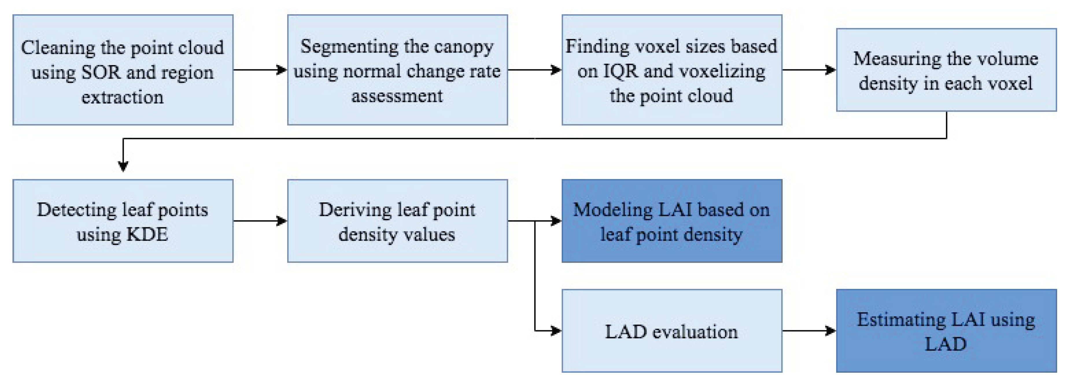
3.1. Point Cloud Denoising

The first pre-processing step involved noise reduction the TLS point cloud data, since the complicated structure of this forest resulted in many noisy returns in the point clouds. For example, the polar scan location right above the scanner is always highly oversampled, due to the various 270${}^{°}$ scans intersecting at this polar region of the hemisphere, as the scanner rotates through 180${}^{°}$ for the full 270${}^{°}$ × 360${}^{°}$ scan. We therefore downsampled the point clouds using an algorithm based on the spherical sampling of the data points, in order to avoid any bias in our data. This technique uses a range-based weighting function, i.e., smaller weights for closer and higher weights for further removed scan locations [27]. Statistical Outlier Removal (SOR) was used as an additional step during the noise reduction process [28]. SOR calculates the distance of each point to its neighbors and removes those that are further away. The distance between the points is compared, based on the average distance between points in the point cloud. The number of neighbors chosen in this research was five, which was obtained based on the density of the points in the vegetation structures we needed to maintain, and it allowed us to preserve these structural components and remove most of the noise points. Next, we used a connected component labeling algorithm for detecting more dense structures and removing irrelevant points, especially in the lower canopy where the structural complexity and the plant/point density were higher. Connected component labeling, which is also known as blob or region extraction, is an algorithm application of graph theory, where segments of connected components are labeled similarly [29]. Connected component labeling detects connected regions in images, and can be used in 3D form for point clouds. This algorithm segments the point cloud into smaller parts that are separated by a minimum distance; in this study, we used a grid size of 0.15 m for our segmentation. This value was chosen based on the point density of the vegetation structures from the lower portion of the point cloud, like stems and ferns. Connected component labeling was effective at removing the irrelvant (noise) lidar points, with the resulting segments including the actual forest structures of interest. This stage was critical because, even after SOR was applied, there were still some noise points remaining in the areas where the point cloud was dense and contained more complex, sub-canopy level, and arguably irrelevant structures, in terms of the study’s objective (LAI estimation).

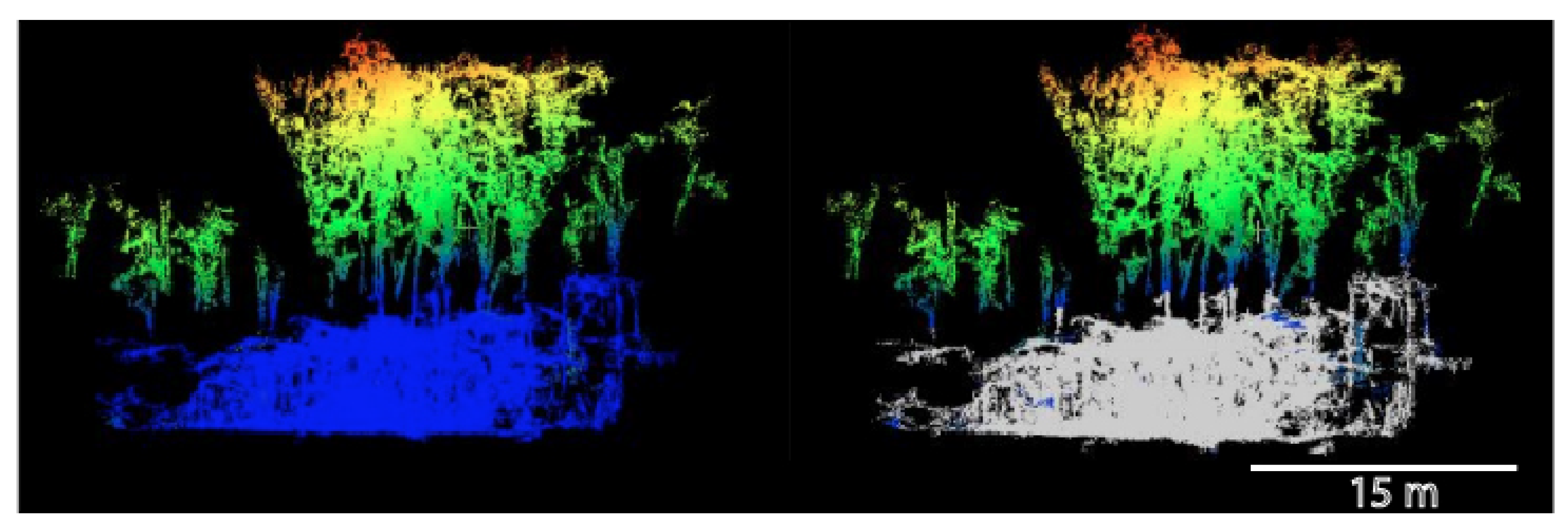
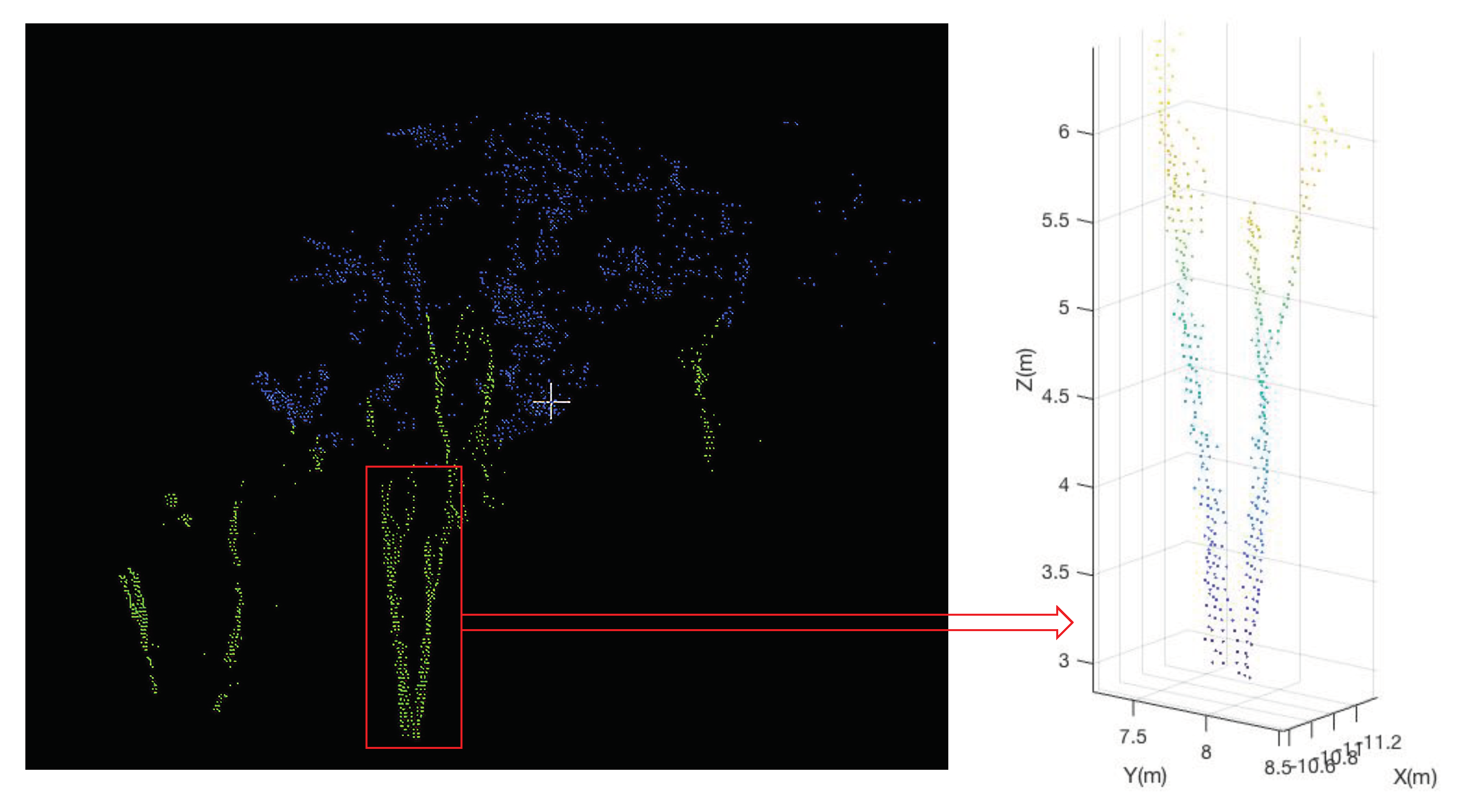
3.2. Detecting the Canopy

Detection of the higher canopy was achieved via normal change rate assessment. As mentioned earlier, the more the surface structure changes in adjacent points in the lidar point cloud, the more their normals are oriented differently, or the more variable these normals become. Figure 3 shows the result of the segmentation of the higher canopy in one of the scans. It is important to mention that, in some of the plots, due to the very complex vegetation structures (e.g., irregular stem or branch shapes), we needed to manually remove some of the points that were incorrectly segmented as higher canopy. This step of the algorithm can in future research be improved by deriving more geometric features for differentiating the canopy from other segments of the point cloud.

3.3. Finding Voxel Sizes

After segmenting the higher canopy regions of the plots, using the previously mentioned normal change rate assessment technique, and in order to perform the voxel-based approach for LAD measurement, we divided the canopy point cloud into layers in the Z direction. Each layer then was divided into other layers in the X direction, in order to decrease the computational time and also the confusion for our algorithm, which can be caused by excessively large numbers of points and a broad density distribution. The number of layers in the Z direction were chosen to be five because this number provided us with a narrower range of density distributions in each layer, where the difference between the maximum and minimum point density was much lower than that for the whole canopy point cloud. This reduces the computational time and confusion for our algorithm. As a result, we can state that:

$$\Delta h=(z_{max}-z_{min})/5,$$

(18)

where $\Delta h$ is the height of each layer, $z_{max}$ is the maximum height of the points in the canopy, and $z_{min}$ is the minimum height of the points segmented as the canopy. Voxel size is a critical parameter that can affect the performance of the algorithm. We observed that larger voxels in the areas with a higher number of points can lead to an underestimation of the number of leaf points, whereas smaller voxels in regions where there are fewer points can lead to an overestimation of the density in these areas. The mentioned factors can introduce extreme outliers into our model. As a result, we determined the voxel sizes in the X direction based on the number of points in each voxel and by using inter-quartile analysis. In each plot, we used the layer containing the highest number of points for finding the voxel sizes. A third degree polynomial, shown by the following equation, was fitted to the density distribution of the layer:

$$f\left(x\right)=p_1{x}^3+p_2{x}^2+p_{3}x+p_4,$$

(19)

where x denotes the X coordinate values of the points. We then used interquartile analysis in order to find the initial size of the voxels. The second quartile ($Q_2$) is the median of the polynomial function. The first and third quartiles ($Q_1$ and $Q_3$) are the medians of the lower and upper half of the dataset, respectively. The Inter-quartile Range (IQR) is described follows:

$$IQR=Q_3-Q_1.$$

(20)

We then calculated the density values that are half the IQR further from the median of the density distribution, $Q_2$:

$$D_1=Q_2-\left(0.5\right)IQR,$$

(21)

$$D_2=Q_2+\left(0.5\right)IQR.$$

(22)

After calculating these density values, we determined their corresponding X values. We call the X value at the median of the density, $x_{median}$, and $x_1$ and $x_2$ are the X values at $D_1$ and $D_2$, respectively. The distance between these X components are described with the following equations:

$$\Delta x_1=|x_1-x_{median}|,$$

(23)

$$\Delta x_2=|x_2-x_{median}|.$$

(24)

We introduce our initial $\Delta x$ as the minimum of these two distances because we want our voxels to be smaller in the areas that contain a large number of points:

$$\Delta x=\min (\Delta x_1,\Delta x_2).$$

(25)

As a result, our first two voxels have the size of $\Delta x$, while the starting point would be $x_{median}$. It should be noted that, since the third degree polynomial may not be monotonous in the range of $0.5\times IQR$ from the median of the density distribution, there can be another condition, i.e., other than a monotonous distribution in that range that has to be considered, where there is a relative maximum in the range of $0.5\times IQR$ from the median. In this case, one of the $D_1$ or $D_2$ values would be the same as Equation (21) or (22), depending on which side of the median the maximum is located. To obtain the other X value, we calculate the difference in the density values of the median and the maximum ($D_{\max }$), and then find the density value equal to $0.5\times IQR-(D_{max}-Q_2)$. Afterwards, we determine the corresponding X value at this density, either higher or lower than the X at the maximum, depending on whether the maximum is on the right or left of the median, respectively.

After determining the width of the first two voxels, we found the number of points in each and introduced the threshold used for detecting the voxel sizes, as the average of these two voxels:

$$N\mathrm{th}=\frac{N_1+N_2}{2},$$

(26)

where $N_1$ and $N_2$ are the number of points in the first two voxels and the Nth is set as the threshold used for finding the voxel sizes in the X direction. The next step involves calculating the width of the voxels based on this threshold, meaning that each voxel should contain a number of points equal to Nth. It is important to mention that, in the far ends of the point cloud, where the point density is significantly lower, if the number of points were less than one third of the threshold ($N\mathrm{th}$), we merged that region with the previous one, thereby forming one voxel. This is due to the fact that a small number of points result in an excessively narrow and inaccurate density distribution.

Table 3. Voxel sizes statistics.

Minimum (m)	Maximum (m)	Mean (m)	Stdev (m)
0.73	3.46	1.57	0.62

shows the statistics for the voxel sizes.

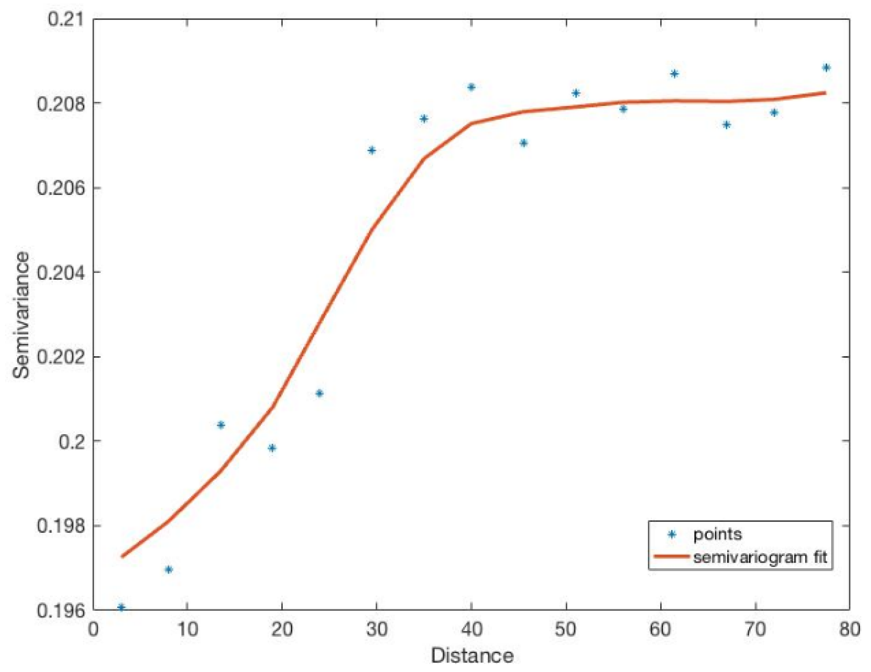
3.4. Measuring the Volume Density

The backscattered power (intensity) from woody materials in the shortwave-infrared (SWIR), i.e., the spectral region roughly between 1400–2500 nm, is higher than the power returned from leaves, due to the liquid water absorption by leaves [30]. The CBL operates at a wavelength of 905 nm, and, although the difference in intensities in foliar and woody materials at 905 nm is not as noticeable as in the SWIR region, there is still a higher intensity recorded for the stems and branches. Additionally, the leaves in the higher canopy of the HAVO site, visible in the lidar point cloud, are mostly flat and horizontally oriented. The scanned area of the leaves decrease dramatically further away from the scanner, multiplied by the cosine of the scan angle. However, due to the cylindrical shape of the branches and their relatively vertical structure, their scanned area is relatively consistent along the scene. The angular distribution of some of the detected branches was found to be between 72${}^{°}$ to 121${}^{°}$, while the angular distribution of the leaves, which was derived from facets of the manually-detected leaf point clouds, was found to be between 11${}^{°}$ and $-{23}^{°}$ [31]. This shows that the leaves are more horizontally oriented in this scene. As a result, we can assume that the total scanned area of the leaves is lower than for the stems and branches, especially in regions further from the scanner.

We also incorporated the images resulting from the intensity images of the point clouds, recorded by the scanner, in order to detect some of the branches and leaves accurately. We were able to detect points that were definitively branches and others that were leaves, purely by detecting the intensity image edges and “outlining” the original image. This was done using the Canny edge detection algorithm [32]. In this approach, a Gaussian filter first is applied to the image to reduce noise, after which the intensity gradient of the image is produced. Non-maximum suppression is applied afterwards to remove the incorrectly detected edges; this algorithm operates by finding the main edges and removing detected edges that do not exhibit a strong connectivity to the main edges. We then measured the density of the detected foliar and woody regions. This was done for twenty plots and 40 segments of leaves and branches in each plot. We found that the density of the branches was higher than that for the leaves by an average order of magnitude of 10 in all of the 20 selected plots. These results support our hypothesis that one will observe a higher lidar point density for branch regions, when compared to foliar materials in TLS point clouds.

Finally, we calculated the volume density, i.e., the number of points in a known volume, in each of the canopy voxels. The first issue is the grid size, which is used for measuring the density. We manually investigated 110 random plots from the original 242 plots. The average width of the biggest branch in the lowest portion of the higher canopy was found to be 0.09 m. Consequently, we chose the grid size to be 0.1 m on each side. In other words, in each of the voxels, the volume density in a 3D grid with the size of 0.1 m was measured.

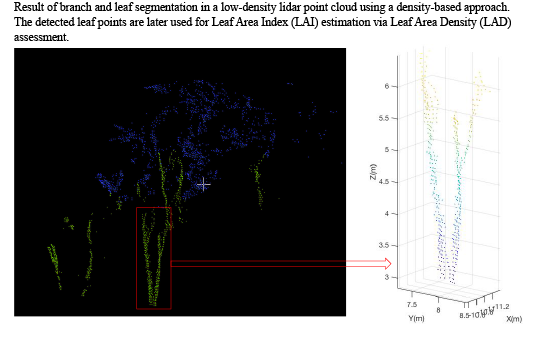
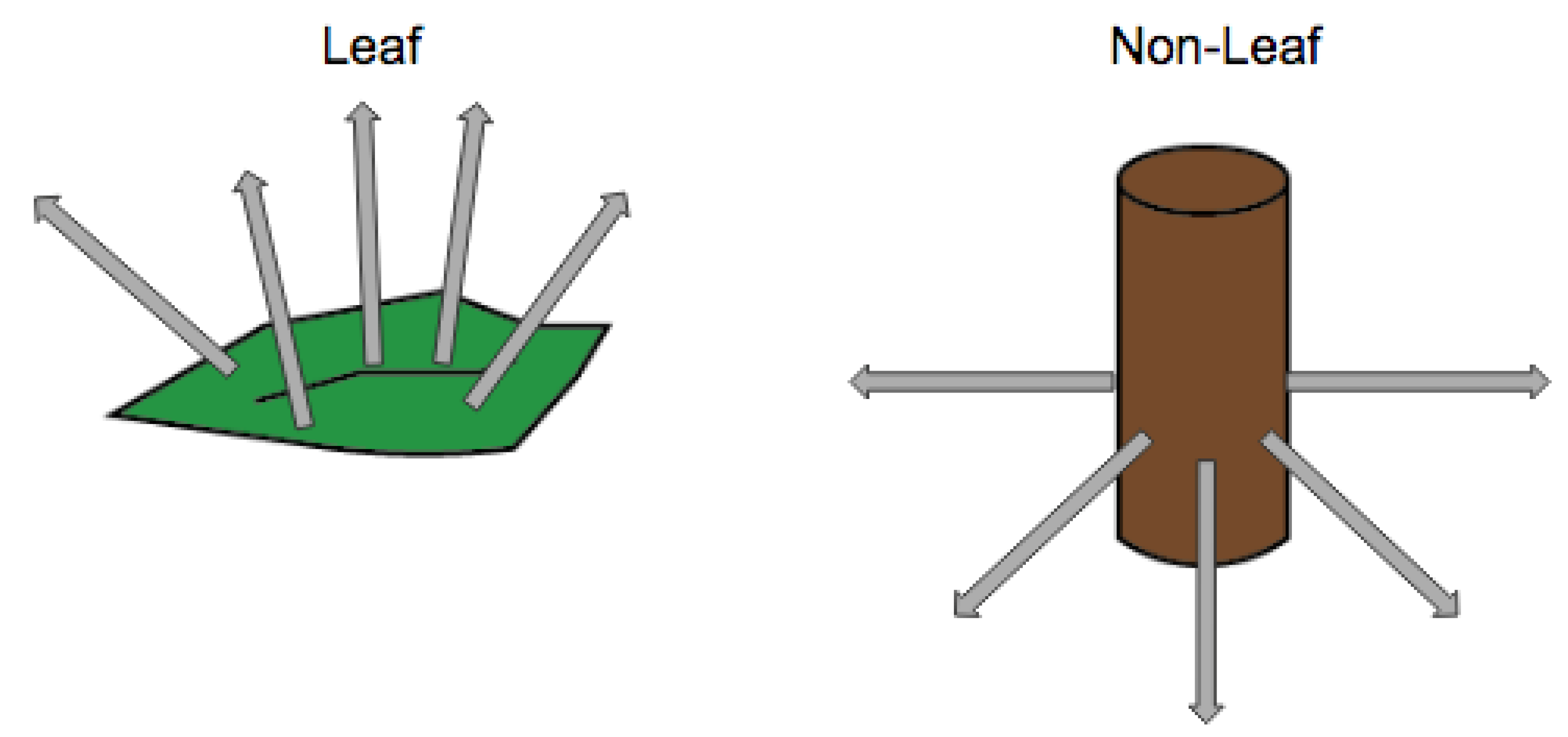
3.5. Detecting Leaf Points

The next stage constitutes a seminal step in the process, namely the segmentation of leaves from branches, accomplished by setting a threshold for the density values in each voxel. We thus fitted a kernel density estimator to the density histogram in each voxel. In probability theory and statistics, Kernel Density Estimation (KDE) is a continuous and non-parametric approach for estimating the probability density function of a random variable [33]. KDE is used when no assumptions are made regarding the form of the data distribution, which is the case in our study. KDE can be estimated using the following formula:

$$f_h(x)=\frac{1}{n}\sum _{i=1}^n{K}_h(x-x_i)=\frac{1}{nh}\sum _{i=1}^{n}K(\frac{x-x_i}{h}),$$

(27)

where n is the number of points, K is the kernel, and h is the bandwidth, which is a smoothing parameter in the KDE formula. The density threshold was obtained based on half of the area under the KDE curve. Figure 4 shows an example from one of the distributions and the threshold chosen, based on the area under the curve.

The points that have lower density values than the threshold are labeled as leaves, while those points above the threshold were labeled as non-leaves (woody material). We modeled the LAI using these leaf point densities, with the results presented in the next section.

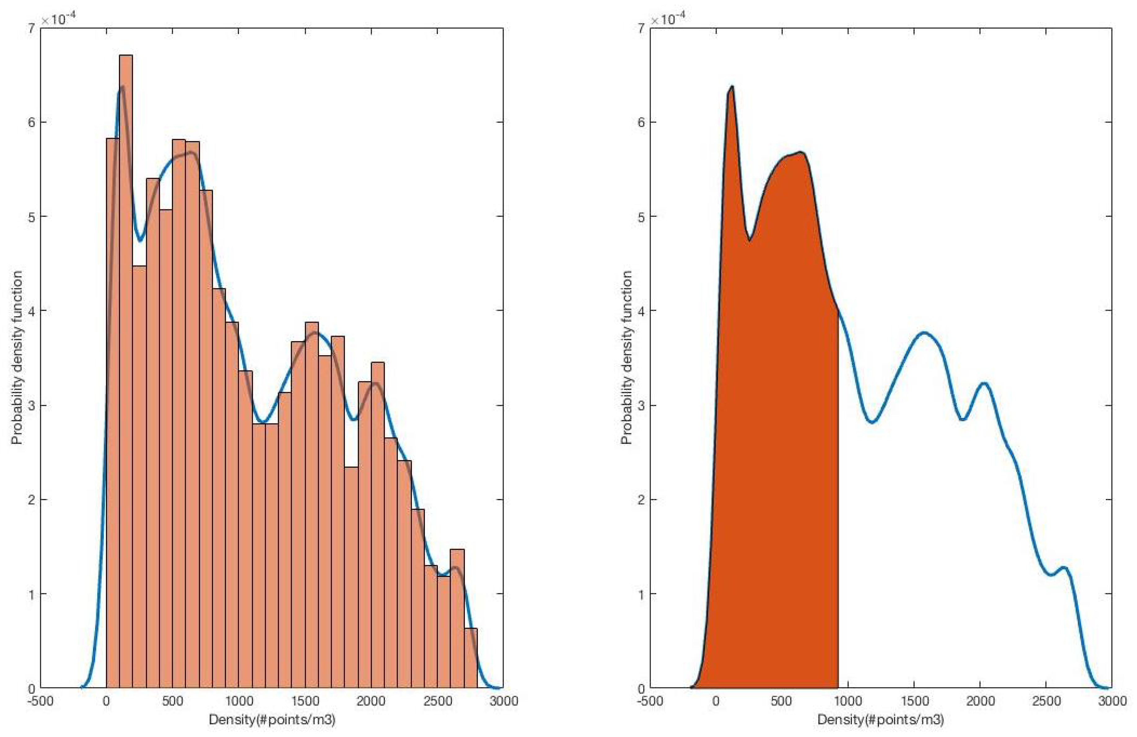
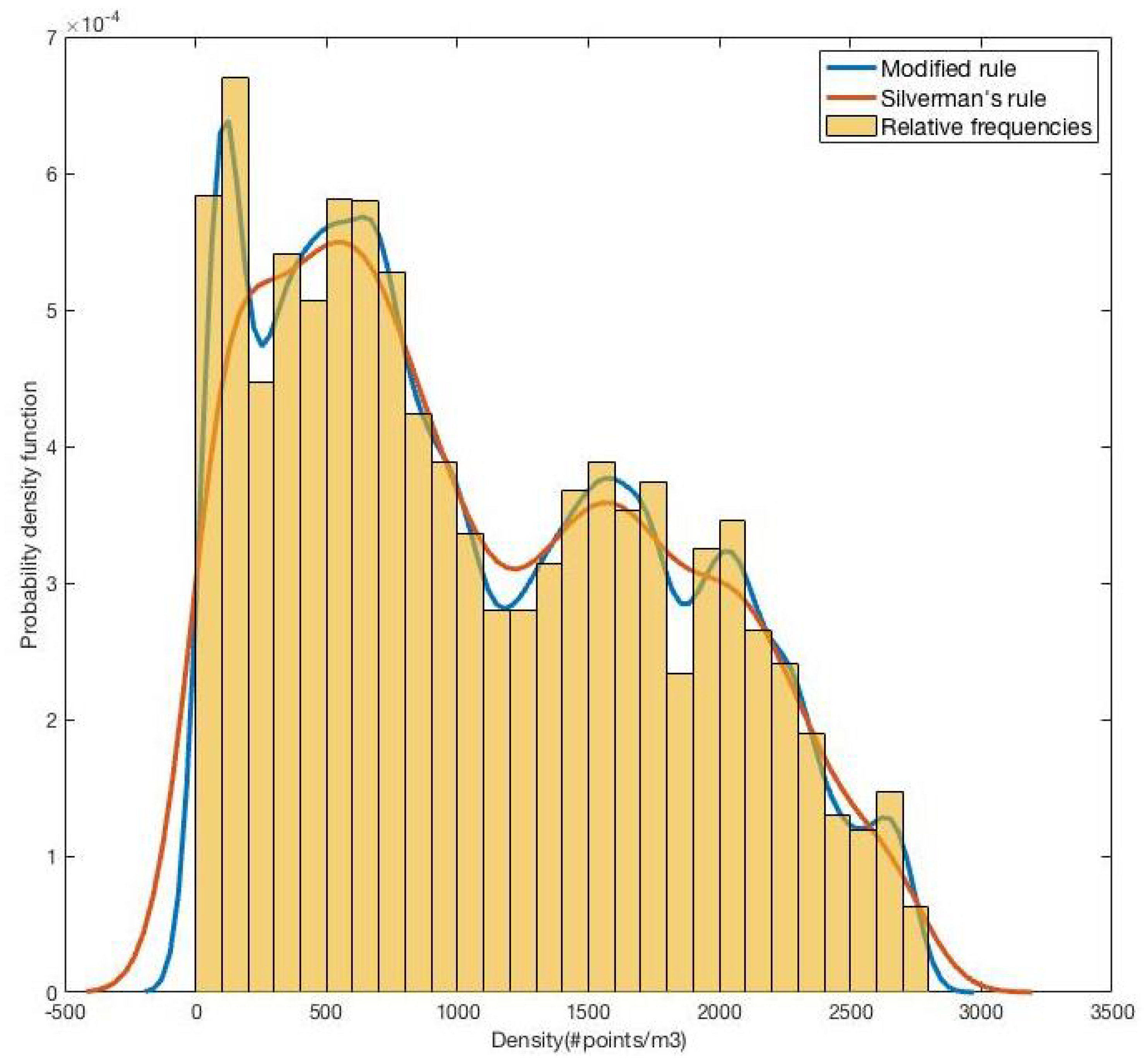
KDE Bandwidth Selection

The bandwidth, or bin size, is an important parameter when using KDE. The bandwidth can be estimated using Silverman’s (1986) rule of thumb. The formula for the bandwidth derived with this method is presented below:

$$h={(4{\sigma }^5/3n)}^{1/5}\approx 1.06\sigma n^{-1/5},$$

(28)

where n is the number of points and $\sigma$ is the standard deviation of the density distribution. Silverman’s rule of thumb is calculated with an assumption of a normal distribution, which is unsuitable for our data. As a result, we reduced the constant value from 1.06 to 0.5 in order to avoid the over-smoothing caused by the normal density assumption. The bandwidth we used in this study therefore is obtained via the following equation:

$$h=0.5\sigma n^{-1/5}.$$

(29)

Figure 5 shows the difference between the two KDEs, one obtained with Silverman’s rule of thumb, and the other one with the modified bandwidth. Figure 6, representing the leaf vs. woody segmentation, shows the result of leaf detection in one voxel using the KDE thresholding.

3.6. LAI Estimation Using LAD

We also calculated the LAI directly from our detected leaf points using the LAD measurement. LAD is calculated as the total one-sided leaf area per unit volume. In the last step, LAI is calculated as sum of the LAD measurements in the layers in the Z direction:

$$LAI={\int }_0^{h}LAD\left(z\right)dz.$$

(30)

In our case, since we have discrete values for different height intervals, we can state:

$$LAI=\sum _{i=1}^{5}LA{D}_i,$$

(31)

where i denotes the number of layers. Figure 7 shows the workflow/diagram of the methods used in this study. The results for modeling the LAI based on (i) the point densities and (ii) the direct derivation of LAI using the LAD estimation are presented in the next section.

4. Results and Discussion

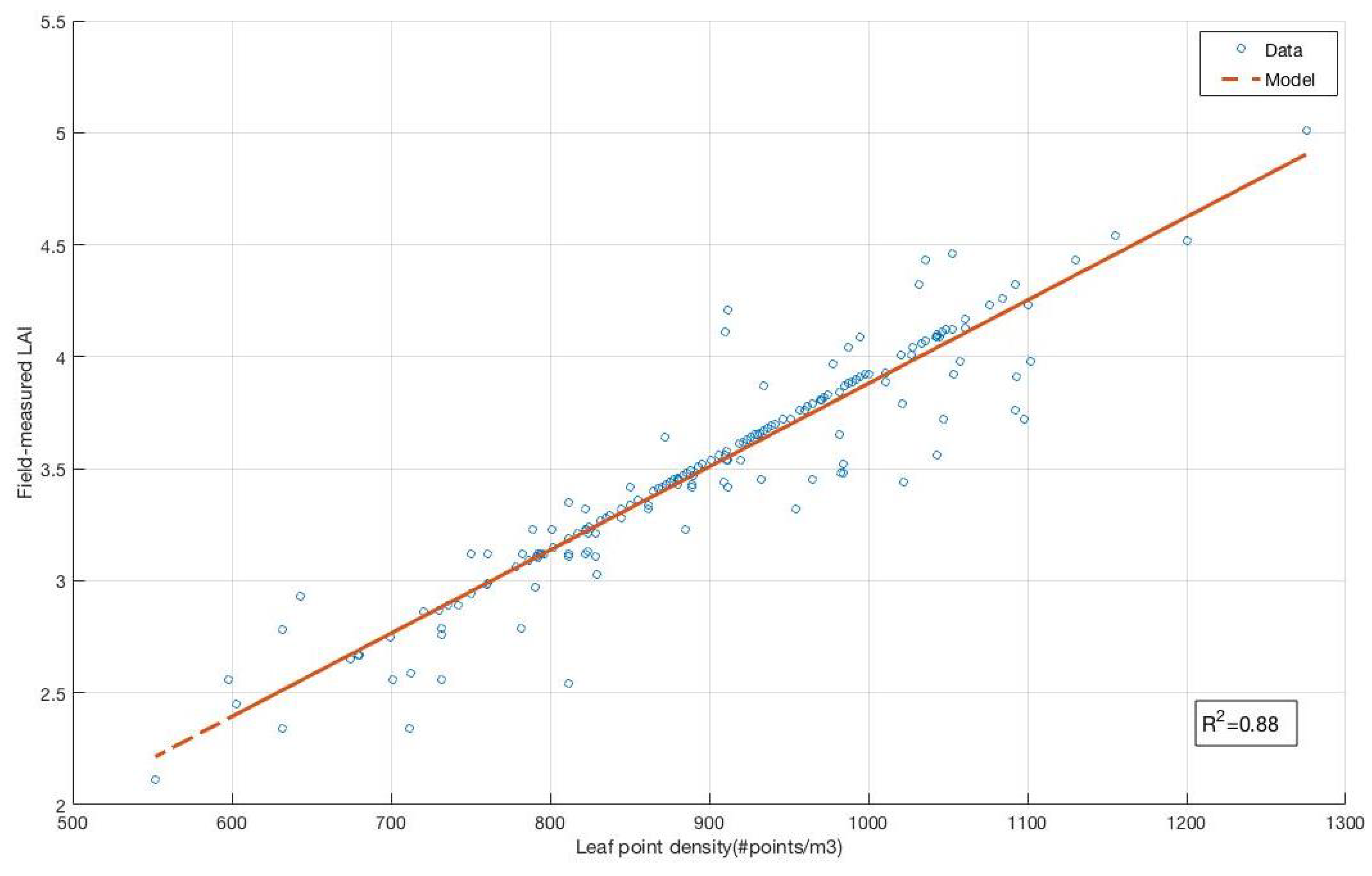
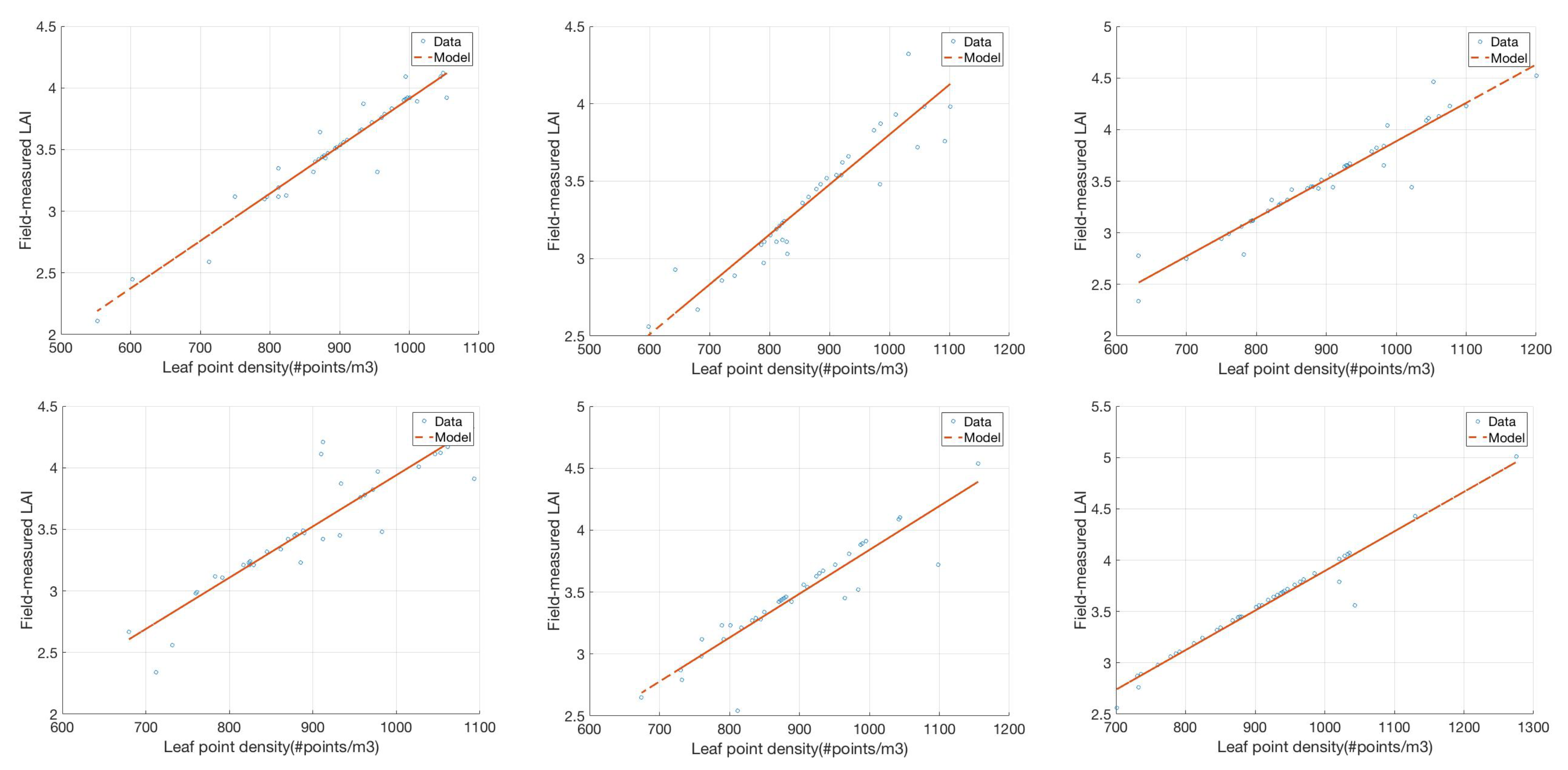
4.1. Results

We followed two approaches in evaluating our algorithm; first, we modeled the field-measured LAIs using the derived leaf point densities, and, second, we directly estimated the LAI using the detected leaf points and LAD assessment. In the case of direct estimation of the LAI values obtained from our TLS data analysis, we ran the algorithm on all 242 plots and achieved an average accuracy of 90%, ranging from 79% to 97%. Accuracy in this case is calculated by directly comparing the field measured LAI and the derived LAI from TLS data in each plot. The following equation is used for assessing the accuracy:

$$Accuracy=\frac{FieldLAI-|FieldLAI-LidarLAI|}{FieldLAI},$$

(32)

where the $FieldLAI$ represents the field-measured LAI using the Accupar LP-80, and the $LidarLAI$ is the TLS-derived LAI value in each plot. The RMSE value for LAI assessment was 0.31, with an overestimation of $9\%$ for the average lidar-derived LAI, compared to the field-measured LAI. We also found the accuracy was lower in the plots where the canopy structural complexity is higher, i.e., the vegetation density is higher in the canopy, especially in the lower portion of the canopy which decreases the lidar beam penetration to the higher levels of the canopy. We refer to “complexity” in this scenario in terms of canopy “density”, i.e., expressed via the number of lidar pulses returned at specific vertical strata throughout the canopy, and their inherent impact on transmission of laser pulses to higher strata; specific examples are provided in the Discussion section. This issue introduces challenges to the leaf detection algorithm and associated LAI estimation. The obtained accuracy shows that this approach can be used for estimating LAI values in a complex forest environment, especially since an error <$10\%$ generally is acceptable in natural resource studies (see [34]).

In the case of modeling the LAI using the leaf point densities, we achieved an $R^2$ value of 0.88. The leaf point densities in each voxel in this case were calculated as the mean of the densities of the points labeled as leaves. Figure 8 shows the linear model obtained from this analysis. However, this latter analysis assumed no spatial auto-correlation between the 5 m-spaced scans, which necessitated an additional step to evaluate the robustness of our approach.

We next performed semi-variogram analysis to evaluate the spatial dependence between the field-measured LAI values, since the field-measured LAI arguably cannot be considered spatially independent across all of the 242 field plots. A semi-variogram is measured for two points separated at a distance of h using the following formula [35]:

$$\gamma \left(h\right)=\frac{1}{2V}{\int \int \int }_V{[f(M+h)-f\left(M\right)]}^{2}dV,$$

(33)

where M is a spatial point in the data, V is the geometric representation of the data, and $f\left(M\right)$ is the value at that point, which in our work is the field-measured LAI. Figure 9 shows the result of the semi-variogram analysis.

We found that the LAI values are spatially independent for plots spaced more than 30 m apart, based on the semi-variogram analysis. Consequently, we divided the 242 plots into six different data sets, each random iteration containing the plots that had a 30-m between-plot spacing. The LAI values in each of these sets were modeled using the derived leaf densities, and the $R^2$ values ranged from 0.84–0.96; Figure 10 shows the six linear models. The linear models for these subsets of data show that the algorithm performs well for the regions, even where the LAI can be considered spatially independent.

4.2. Discussion

The presented approach provides a method for automatic leaf detection and LAI assessment, an important parameter in structural evaluation of vegetation, for what could be considered complex forest environments. This algorithm reduces the time and cost associated with data collection for LAI assessment, and provides the ability to assess canopy-level structural attributes, which can be manually impractical due to the structural complexity of many forest environments. This study therefore contributes to plot-level assessment of canopy structural attributes, such as LAI and LAD, using a low-cost, portable TLS, and it does so at high accuracy and precision rates. While previous studies have shown that the higher-density TLS data can provide accurate estimations of LAI, using geometrical attributes of the canopy and directional gap fraction assessment [36,37], the lower-density data used in this work, in terms of lower angular resolution of the scanner and lower associated lidar point density, reduce the cost and time of data collection. However, low-density data make the derivation of geometric traits of the leaves and branches difficult and introduce associated challenges to structural assessment via TLS data. As an example, Antonarakis et al. [36] used a directional gap fraction approach to estimate LAI using TLS in three forests which consisted mostly of commercial hybrid poplars. While this method proved to be effective when using high-density data, low-density data do not allow an accurate assessment of canopy gap fraction, due to an inability to capture geometric characteristics of the intra-canopy structures, i.e., leaves and branches, and to evaluate their impact on the radiation transferred through the canopy. Our approach thus uses only one variable, namely lidar point density, to detect leaves, and to evaluate LAD and LAI. The lidar point densities are obtained using statistical analysis of the canopy lidar point cloud, without the need of additional geometric and structural parameters. In addition to the issues caused by low-density data, the structural complexity of the studied tropical forests, i.e., the vegetation density and associated lidar point density in the canopy at different vertical strata, introduces challenges to plot-level LAI assessment, when compared to evaluating LAI using a controlled laboratory experiment (e.g., [38]), or a single tree scan (e.g., [39]). Li et al. [39] developed a point cloud slicing approach based on the canopy gap fraction, and were successful in estimating LAI using a single-tree scan. Although an approach like the one used in our work may not provide results as accurate as the ones obtained using methods based on high-density data and single tree scans, our method estimates plot-level LAI, thus reduces the time and cost of data collection, which results in more practical applications of TLS in forest inventories. In another study, Olsoy et al. [40] used TLS to model LAI in 42 Wyoming big sagebrush shrubs, using canopy cover, the percentage of the total ground area which is covered by the vertical projection of the tree crown, and canopy volume as TLS variables. They acquired an $R^2$ value of 0.73 for modeling LAI using canopy cover and an $R^2$ of 0.78 when modeling LAI using the canopy volume obtained based on a convex hull approach. Such a method can be effective in assessing LAI using small-range TLS data and single tree scans, while in our work we addressed these issues by developing a density-based approach for assessing the plot-level LAI, acquiring $R^2$ values in the range of 0.84 to 0.96. Additionally, the accuracy of canopy volume estimation can decrease when the structural complexity and vegetation density increases, and also in further ranges from the scanner, due to lower penetration rate of lidar pulses in those regions and lower associated lidar point density [41]. TLS data and voxel-based approaches, like the one presented in our work, also have been used for LAI assessment in relatively recent studies. Greaves et al. [42] used a voxel counting approach for LAI estimation in low-stature (<1.5 m tall) Arctic shrub species. In this method, the TLS point cloud is divided into voxels, and then the number of voxels that are occupied by at least one point are counted and the number of these voxels per unit ground area provides the LAI estimate ($R^2$ = 0.94 for close range (2 m) TLS data). While this approach is successful in LAI estimation of low-stature species, TLS data used in our work are from tropical forests with the maximum TLS point cloud height ranging from 13 m to 18 m. As a result, such a method, solely based on voxel counting, can in fact lead to PAI, instead of LAI, due to the inability to differentiate between leaves and branches. Zheng et al. [43] found that the nonphotosynthetic canopy components, e.g., branches, contributed from 19% to 54% to LAI estimation depending on canopy vegetation densities. Therefore, the density-based approach presented in our work for detecting leaves in low-density data increases the plot-level LAI estimation accuracy in forest environments with dense vegetation, such as tropical forests.

We did, however, observe an overestimation of 9% for the average lidar-derived LAI, compared to the field-measured LAI. This slight discrepancy was partly attributed to the fact that the field-measured LAI is highly dependent on the spatial characteristics of the location where the measurement is collected, while the TLS-derived LAI depends on the overall canopy-level spatial and structural attributes. Although the algorithm proved effective in achieving its objective, the performance is affected by the structural complexity in the canopy point cloud, specifically vegetation density. It was found that the accuracy of LAI estimation decreases, coupled to increases in vegetation density, especially in the lower part of the canopy. These more complex, higher density lower-canopy regions effectively reduce the penetration rate of lidar pulses to the higher regions of the canopy, thereby resulting in associated lower LAI assessment accuracy. As an example, in the plot where we obtained the lowest LAI estimation accuracy, 79%, the point density of the lowest layer in the Z direction was 2.21 times the second lowest layer, and the density in the second lowest layer was 1.74 times the third one. This results in a distinct decrease in lidar point density in different height levels of the canopy, which is a result of lower lidar beam penetration due to higher vegetation density in the canopy, whereas, in the plot in which we acquired the highest accuracy of LAI estimation, 97%, the point density of the lowest layer in Z direction was 1.19 times the second lowest layer, and the point density of the second lowest layer was 1.22 of the third one. This shows that, in such plots, there is a higher point density throughout the whole canopy point cloud, which results in a more accurate estimation of LAI. To address this issue, future research can incorporate a fusion of airborne lidar and TLS data to mitigate the impact of lower-canopy structural complexity on lidar pulse penetration throughout the canopy, and thereby hypothetically increase the accuracy of such LAI assessment approaches.

We also showed that a robust approach, i.e., one that incorporates spatial auto-correlation considerations, did not result in significantly poorer LAI assessment performance. In fact, our full 242 plot set $R^2$ value of 0.88 for LAI modeling represented the range of $R^2$ values for the spatially-uncorrelated sets ($R^2$ = 0.84–0.96). This implies that, in practice, one could optimize or improve LAI assessments by evaluating the spatial auto-correlation of canopy structure variables, and then develop statistically-reliable, valid estimates for the main parameter of interest (LAI). It also could be argued that such an approach improved estimates, i.e., we achieved $R^2$ values as high as 0.96, by constraining our modeling to spatially-independent regions within the forest. We therefore recommend that future efforts also include an investigation into how such a spatial statistics approach applies to potential predictor variables, such as leaf density, gap fraction, etc., over and above the dependent variable (LAI).

Future research, over and above the previously-mentioned topics, can include the use of a dual- or multi-wavelength scanner in order to better differentiate foliar and woody materials and thereby improve algorithm performance. If the scanner wavelength is located in the SWIR spectral region, e.g., 1520 nm, we expect to see a better separation between the leaf and non-leaf (woody) segments. This is due to the larger difference in moisture-impacted reflectance values of these two materials in the SWIR wavelength range. As an example, Zhao et al. [44] used the dual wavelength Echidna lidar (DWEL; [30]), which collects data in two different wavelengths (1064 nm and 1548 nm), to measure the effective LAI. Such a system typically enables better discrimination between reflectance values of woody and foliar materials in the canopy, due to its ability to collect lidar data in the SWIR spectral region. The Echidna also yields higher density point clouds, with an angular step width of approximately 1 mrad, compared to the discrete lidar system used in this work, the CBL, with a minimum angular step width of 4.6 mrad.

5. Conclusions

We presented an algorithm for modelling and estimating the LAI in a complex, tropical forest environment using lidar point densities, derived from TLS data. The data used in this study were from a portable (3.2 kg), rapid-scan (33 s), low-cost (USD 20,000) TLS system. We assumed that the intensity (or power) returned to the scanner from woody materials is higher than for the leaves at 905 nm, and supported this hypothesis by investigating the point cloud density, both in foliar and woody segments. We acquired an accuracy of 90%, and RMSE value of 0.31 in directly estimating the field-measured LAI, using LAD assessment, and $R^2$ values of 0.84–0.96 for modeling the field-measured LAI with leaf point density values, for spatially-uncorrelated plot locations. An overestimation of $9\%$ was found in the TLS-derived LAI compared to the field-measured LAI. This was attributed to the fact that TLS-derived LAI considers overall canopy-level structural attributes, while the field-measured LAI is sensitive to the spatial characteristics (angular canopy interactions, illumination conditions, etc.) of the specific location where the LAI is measured. The data in this study were from an arguably complex forest type, which makes each step of this approach more challenging. However, this algorithm works well in predicting the LAI using just one variable, namely leaf point density. We also considered the fact that the LAI values may not be spatially independent across the whole scene. As a result, by using semi-variogram analysis, we found that this approach works well for spatially-independent LAI values as well. This algorithm works well for automatic detection of leaf points in lower-density TLS lidar data. However, when higher-density (small angular resolution, high point density) lidar data are available, the geometric information of the leaves and branches potentially can be used to improve the leaf detection algorithm.

This algorithm can be used for evaluating LAI in complex forest environments and when derivation of the geometric information and structure from the data are not practicable, due to low scanner angular resolution (and associated point cloud densities) or limited structural retrievals of the scanned site. Finally, such a rapid-scan, fine-scale approach to LAI assessment could prove useful to the larger community when it comes to calibration/validation of landscape-to-regional scale products, derived from airborne- and spaceborne platforms.

References

1. Chen, J.M.; Rich, P.M.; Gower, S.T.; Norman, J.M.; Plummer, S. Leaf area index of boreal forests: Theory, techniques, and measurements. J. Geophys. Res. Atmos. 1997, 102, 29429–29443. [Google Scholar] [CrossRef]
2. Whitehead, D.; Hinckley, T.M. Models of water flux through forest stands: Critical leaf and stand parameters. Tree Physiol. 1991, 9, 35–57. [Google Scholar] [CrossRef] [PubMed]
3. Amthor, J.S.; Gill, D.S.; Bormann, F.H. Autumnal leaf conductance and apparent photosynthesis by saplings and sprouts in a recently disturbed northern hardwood forest. Oecologia 1990, 84, 93–98. [Google Scholar] [CrossRef] [PubMed]
4. Davi, H.; Soudani, K.; Deckx, T.; Dufrene, E.; Le Dantec, V.; Francois, C. Estimation of forest leaf area index from SPOT imagery using NDVI distribution over forest stands. Int. J. Remote Sens. 2006, 27, 885–902. [Google Scholar] [CrossRef]
5. Wilhelm, W.W.; Ruwe, K.; Schlemmer, M.R. Comparison of three leaf area index meters in a corn canopy. Crop Sci. 2000, 40, 1179–1183. [Google Scholar] [CrossRef]
6. Chen, Q.; Baldocchi, D.; Gong, P.; Kelly, M. Isolating individual trees in a savanna woodland using small footprint lidar data. Photogramm. Eng. Remote Sens. 2006, 72, 923–932. [Google Scholar] [CrossRef]
7. Morsdorf, F.; Kötz, B.; Meier, E.; Itten, K.I.; Allgöwer, B. Estimation of LAI and fractional cover from small footprint airborne laser scanning data based on gap fraction. Remote Sens. Environ. 2006, 104, 50–61. [Google Scholar] [CrossRef]
8. Martens, S.N.; Ustin, S.L.; Rousseau, R.A. Estimation of tree canopy leaf area index by gap fraction analysis. For. Ecol. Manag. 1993, 61, 91–108. [Google Scholar] [CrossRef]
9. Jarvis, P.G.; Leverenz, J.W. Productivity of temperate, deciduous and evergreen forests. In Physiological Plant Ecology IV; Springer: Berlin/Heidelberg, Germany, 1983; pp. 233–280. [Google Scholar]
10. Henning, J.G.; Radtke, P.J. Detailed stem measurements of standing trees from ground-based scanning lidar. For. Sci. 2006, 52, 67–80. [Google Scholar]
11. Li, S.; Dai, L.; Wang, H.; Wang, Y.; He, Z.; Lin, S. Estimating leaf area density of individual trees using the point cloud segmentation of terrestrial LiDAR data and a voxel-based model. Remote Sens. 2017, 9, 1202. [Google Scholar] [CrossRef]
12. Jonckheere, I.; Fleck, S.; Nackaerts, K.; Muys, B.; Coppin, P.; Weiss, M.; Baret, F. Review of methods for in situ leaf area index determination: Part I. Theories, sensors and hemispherical photography. Agric. For. Meteorol. 2004, 121, 19–35. [Google Scholar] [CrossRef]
13. Hosoi, F.; Omasa, K. Factors contributing to accuracy in the estimation of the woody canopy leaf area density profile using 3D portable lidar imaging. J. Exp. Bot. 2007, 58, 3463–3473. [Google Scholar] [CrossRef] [PubMed] [Green Version]
14. Béland, M.; Baldocchi, D.D.; Widlowski, J.L.; Fournier, R.A.; Verstraete, M.M. On seeing the wood from the leaves and the role of voxel size in determining leaf area distribution of forests with terrestrial LiDAR. Agric. For. Meteorol. 2014, 184, 82–97. [Google Scholar] [CrossRef]
15. Wilson, J.W. Analysis of the spatial distribution of foliage by two-dimensional point quadrats. New Phytol. 1959, 58, 92–99. [Google Scholar] [CrossRef]
16. Chen, J.M.; Black, T.A.; Adams, R.S. Evaluation of hemispherical photography for determining plant area index and geometry of a forest stand. Agric. For. Meteorol. 1991, 56, 129–143. [Google Scholar] [CrossRef]
17. Omasa, K.; Hosoi, F.; Konishi, A. 3D lidar imaging for detecting and understanding plant responses and canopy structure. J. Exp. Bot. 2006, 58, 881–898. [Google Scholar] [CrossRef] [PubMed] [Green Version]
18. Tao, S.; Wu, F.; Guo, Q.; Wang, Y.; Li, W.; Xue, B.; Hu, X.; Li, P.; Tian, D.; Li, C.; et al. Segmenting tree crowns from terrestrial and mobile LiDAR data by exploring ecological theories. ISPRS J. Photogramm. Remote Sens. 2015, 110, 66–76. [Google Scholar] [CrossRef] [Green Version]
19. Ghebrezgabher, M.G.; Yang, T.; Yang, X.; Wang, X.; Khan, M. Extracting and analyzing forest and woodland cover change in Eritrea based on landsat data using supervised classification. Egypt. J. Remote Sens. Space Sci. 2016, 19, 37–47. [Google Scholar] [CrossRef] [Green Version]
20. Woo, H.; Kang, E.; Wang, S.; Lee, K.H. A new segmentation method for point cloud data. Int. J. Mach. Tools Manuf. 2002, 42, 167–178. [Google Scholar] [CrossRef]
21. Yao, W.; Hinz, S.; Stilla, U. Object extraction based on 3D-segmentation of lidar data by combining mean shift with normalized cuts: Two examples from urban areas. In Proceedings of the 2009 Joint Urban Remote Sensing Event, Shanghai, China, 20–22 May 2009. [Google Scholar]
22. Kelbe, D.; van Aardt, J.; Romanczyk, P.; van Leeuwen, M.; Cawse-Nicholson, K. Single-scan stem reconstruction using low-resolution terrestrial laser scanner data. IEEE J. Sel. Top. Appl. Earth Obs. Remote Sens. 2015, 8, 3414–3427. [Google Scholar] [CrossRef]
23. Vitousek, P.M.; Walker, L.R.; Whiteaker, L.D.; Matson, P.A. Nutrient limitations to plant growth during primary succession in Hawaii Volcanoes National Park. Biogeochemistry 1993, 23, 197–215. [Google Scholar] [CrossRef]
24. Giambelluca, T.W.; Martin, R.E.; Asner, G.P.; Huang, M.; Mudd, R.G.; Nullet, M.A.; Foote, D. Evapotranspiration and energy balance of native wet montane cloud forest in Hawai‘i. Agric. For. Meteorol. 2009, 149, 230–243. [Google Scholar] [CrossRef]
25. Van der Zande, D.; Hoet, W.; Jonckheere, I.; van Aardt, J.; Coppin, P. Influence of measurement set-up of ground-based LiDAR for derivation of tree structure. Agric. For. Meteorol. 2006, 141, 147–160. [Google Scholar] [CrossRef]
26. SICK. LMS100/111/120/151 Laser Measurement Systems Operating Instructions; SICK AG Waldkirch: Reute, Germany, 2009. [Google Scholar]
27. Van Aardt, J.A.; Kelbe, D.; Sacca, K.; Giardina, C.P.; Selmants, P.C.; Litton, C.M.; Asner, G.P. A terrestrial lidar’s assessment of climate change impacts on forest structure. In Proceedings of the Silvilaser 2017, Blacksburg, VA, USA, 10–12 October 2017. [Google Scholar]
28. Rusu, R.B.; Marton, Z.C.; Blodow, N.; Dolha, M.; Beetz, M. Towards 3D point cloud based object maps for household environments. Robot. Auton. Syst. 2008, 56, 927–941. [Google Scholar] [CrossRef]
29. Samet, H.; Tamminen, M. Efficient component labeling of images of arbitrary dimension represented by linear bintrees. IEEE Trans. Pattern Anal. Mach. Intell. 1988, 10, 579–586. [Google Scholar] [CrossRef]
30. Douglas, E.S.; Strahler, A.; Martel, J.; Cook, T.; Mendillo, C.; Marshall, R.; Yang, X. DWEL: A dual-wavelength echidna lidar for ground-based forest scanning. In Proceedings of the 2012 IEEE International Geoscience and Remote Sensing Symposium, Munich, Germany, 22–27 July 2012; pp. 4998–5001. [Google Scholar]
31. Dewez, T.J.; Girardeau-Montaut, D.; Allanic, C.; Rohmer, J. Facets: A Cloudcompare Plugin to Extract Geological Planes from Unstructured 3D Point Clouds. Int. Arch. Photogramm. Remote Sen. Spat. Inf. Sci. 2016, 41, 799–804. [Google Scholar] [CrossRef]
32. Canny, J. A computational approach to edge detection. In Readings in Computer Vision; Morgan Kaufmann: Burlington, MA, USA, 1987; pp. 184–203. [Google Scholar]
33. Parzen, E. On estimation of a probability density function and mode. Ann. Math. Stat. 1962, 33, 1065–1076. [Google Scholar] [CrossRef]
34. Burkhart, H.E.; Avery, T.E.; Bullock, B.P. Forest Measurements, 6th ed.; Waveland Press: Long Grove, IL, USA, 2019. [Google Scholar]
35. Matheron, G. Principles of geostatistics. Econ. Geol. 1963, 58, 1246–1266. [Google Scholar] [CrossRef]
36. Antonarakis, A.S.; Richards, K.S.; Brasington, J.; Muller, E. Determining leaf area index and leafy tree roughness using terrestrial laser scanning. Water Resour. Res. 2010. [Google Scholar] [CrossRef]
37. Danson, F.M.; Hetherington, D.; Morsdorf, F.; Koetz, B.; Allgower, B. Three-dimensional forest cannopy structure from terrestrial laser scanning. Koukal Schneider 2006, 13, 61–65. [Google Scholar]
38. Moorthy, I.; Miller, J.R.; Hu, B.; Chen, J.; Li, Q. Retrieving crown leaf area index from an individual tree using ground-based lidar data. Can. J. Remote Sens. 2008, 34, 320–332. [Google Scholar]
39. Li, Y.; Guo, Q.; Su, Y.; Tao, S.; Zhao, K.; Xu, G. Retrieving the gap fraction, element clumping index, and leaf area index of individual trees using single-scan data from a terrestrial laser scanner. ISPRS J. Photogramm. Remote Sens. 2017, 130, 308–316. [Google Scholar] [CrossRef]
40. Olsoy, P.J.; Mitchell, J.J.; Levia, D.F.; Clark, P.E.; Glenn, N.F. Estimation of big sagebrush leaf area index with terrestrial laser scanning. Ecol. Indic. 2016, 61, 815–821. [Google Scholar] [CrossRef]
41. Watt, P.J.; Donoghue, D.N.M. Measuring forest structure with terrestrial laser scanning. Int. J. Remote Sens. 2005, 26, 1437–1446. [Google Scholar] [CrossRef]
42. Greaves, H.E.; Vierling, L.A.; Eitel, J.U.; Boelman, N.T.; Magney, T.S.; Prager, C.M.; Griffin, K.L. Estimating aboveground biomass and leaf area of low-stature Arctic shrubs with terrestrial LiDAR. Remote Sens. Environ. 2015, 164, 26–35. [Google Scholar] [CrossRef]
43. Zheng, G.; Ma, L.; He, W.; Eitel, J.U.; Moskal, L.M.; Zhang, Z. Assessing the contribution of woody materials to forest angular gap fraction and effective leaf area index using terrestrial laser scanning data. IEEE Trans. Geosci. Remote Sens. 2015, 54, 1475–1487. [Google Scholar] [CrossRef]
44. Zhao, F.; Yang, X.; Schull, M.A.; Román-Colón, M.O.; Yao, T.; Wang, Z.; Newnham, G.J. Measuring effective leaf area index, foliage profile, and stand height in New England forest stands using a full-waveform ground-based lidar. Remote Sens. Environ. 2011, 115, 2954–2964. [Google Scholar] [CrossRef]
Figure 1. Normals of a point cloud of leaf and non-leaf materials. The arrows show the normals of the point cloud. It can be seen that the normal change rate theoretically is higher in leaves compared to more homogeneous woody segments, like branches and stems.
Remotesensing 11 01791 g001
Figure 2. Hawaii Volcanoes National Park (HAVO) site, in which the data were collected for this study. It can be seen that this is a complex forest environment due to the complicated vegetation structures and variations.
Remotesensing 11 01791 g002
Figure 3. The normal change rate assessment for detecting the higher canopy of the point cloud. The image on the left shows the original point cloud after noise reduction, and the image on the right shows the result of normal change rate assessment. It can be seen that the higher canopy is segmented from the lower portion of the scan, where the main part of the trunks and some of the lower ferns are located.
Remotesensing 11 01791 g003
Figure 4. The curve on the left shows the KDE fitted to the density distribution from one of the voxels. The curve on the right shows the threshold found for this distribution. The orange area is the area containing the leaf points’ density values.
Remotesensing 11 01791 g004
Figure 5. The orange curve is the one produced using the bandwidth obtained by Silverman’s rule of thumb, while the blue curve is derived from the modified bandwidth equation. The over-smoothing effect, which is caused by the normal distribution assumption, is visible in this figure, showing that the bandwidth, derived using the modified equation, represents the behavior of the density distribution as a more accurate fit.
Remotesensing 11 01791 g005
Figure 6. This image shows the result of the segmentation of leaves and branches. The green points represent the branches, while the blue points show the leaves. The image on the right depicts the isolated branch point cloud.
Remotesensing 11 01791 g006
Figure 7. A diagram outlining the methods used in this work.
Remotesensing 11 01791 g007
Figure 8. The linear model of LAI using the TLS derived leaf densities. The X-variable represents the point densities, and the y-axis denotes the field LAI measurements. The R 2 value for this model is 0.88, with a standard error of 0.14.
Remotesensing 11 01791 g008
Figure 9. The semi-variogram analysis shows that the LAI values can be considered spatially independent for plots that are spaced at least 30 m apart.
Remotesensing 11 01791 g009
Figure 10. Linear models acquired for the six random sets with plots spaced 30 m apart. The R 2 value for these models ranged between 0.84–0.96, representing a good fit in all the regions. The standard error ranged between 0.05–0.18.
Remotesensing 11 01791 g010