Copernicus Imaging Microwave Radiometer (CIMR) Benefits for the Copernicus Level 4 Sea-Surface Salinity Processing Chain

Abstract

We present a study on the potential of the Copernicus Imaging Microwave Radiometer (CIMR) mission for the global monitoring of Sea-Surface Salinity (SSS) using Level-4 (gap-free) analysis processing. Space-based SSS are currently provided by the Soil Moisture and Ocean Salinity (SMOS) and Soil Moisture Active Passive (SMAP) satellites. However, there are no planned missions to guarantee continuity in the remote SSS measurements for the near future. The CIMR mission is in a preparatory phase with an expected launch in 2026. CIMR is focused on the provision of global coverage, high resolution sea-surface temperature (SST), SSS and sea-ice concentration observations. In this paper, we evaluate the mission impact within the Copernicus Marine Environment Monitoring Service (CMEMS) SSS processing chain. The CMEMS SSS operational products are based on a combination of in situ and satellite (SMOS) SSS and high-resolution SST information through a multivariate optimal interpolation. We demonstrate the potential of CIMR within the CMEMS SSS operational production after the SMOS era. For this purpose, we implemented an Observing System Simulation Experiment (OSSE) based on the CMEMS MERCATOR global operational model. The MERCATOR SSSs were used to generate synthetic in situ and CIMR SSS and, at the same time, they provided a reference gap-free SSS field. Using the optimal interpolation algorithm, we demonstrated that the combined use of in situ and CIMR observations improves the global SSS retrieval compared to a processing where only in situ observations are ingested. The improvements are observed in the 60% and 70% of the global ocean surface for the reconstruction of the SSS and of the SSS spatial gradients, respectively. Moreover, the study highlights the CIMR-based salinity patterns are more accurate both in the open ocean and in coastal areas. We conclude that CIMR can guarantee continuity for accurate monitoring of the ocean surface salinity from space.

1. Introduction

The salinity of the ocean is a crucial parameter to investigate the water cycle, the ocean dynamics and the marine biogeochemistry from the global to the regional scale. It was classified as an Essential Climate Variable in the context of the Global Climate Observing System (GCOS) programme. Indeed, salinity affects both the sea water density and the marine carbonate chemistry (alkalinity), making it a fundamental variable to investigate the thermohaline global circulation, the local surface and deep circulation, the water mass transformation and the uptake of carbon by the ocean including ocean acidification, e.g., [1,2,3,4].

In the past, salinity has suffered from poor observational coverage, being uniquely sampled via point-wise in situ observations, impacting the accurate assessment of its spatial variability and dynamics, in particular for the construction of gap-free optimally interpolated fields, e.g., the in situ-Based Reanalysis of the Global Ocean Temperature and Salinity (ISAS) [5]. The three-dimensional ISAS dataset was recently improved using quasi-global ARGO floats observations [6]. In addition, the characterization of the sea-surface salinity (SSS) has benefited from satellite observations and on their synergy with in situ measurements, e.g., [7,8,9].

In the framework of the Copernicus Marine Environment Monitoring Service (CMEMS), a daily, mesoscale resolving SSS multi-year gap-free Level-4 analysis (L4 hereinafter) product was developed by Buongiorno Nardelli et al. 2016 [10] and Drogheiet al. 2018 [11]. The approach of [10,11], unlike [5,6,7,8,9], relies on a multi-dimensional (multivariate) optimal interpolation (OI) algorithm that combines both Soil Moisture Ocean Salinity (SMOS) satellite retrievals and in situ salinity measurements with satellite sea-surface temperature information. This product is distributed operationally in near real time in late 2018. Despite the success of this product, there are no missions planned to secure continuity of satellite SSS measurements after the SMOS and Soil Moisture Active Passive (SMAP) missions, which could impact both the accuracy and the effective resolution of the CMEMS SSS operational products.

The Copernicus Imaging Microwave Radiometer (CIMR) satellite mission [12] is being developed as a High Priority candidate Mission (HPCM) in the context of the European Copernicus Expansion Programme. To address the needs of Copernicus and the Integrated European Policy for the Arctic, the CIMR mission will carry a wide-swath (>1900 km) conically scanning multi-frequency microwave radiometer. CIMR measurements will be made over a forward scan arc followed ≃260 s later by a second measurement over a backward scan arc. Polarised (H and V) channels centered at 1.414, 6.925, 10.65, 18.7 and 36.5 GHz are included in the mission design under study (full Stokes parameters are foreseen). The real-aperture resolution of the 6.925/10.65 GHz channels is <15 km and 5/4 km for the 18.7/36.5 GHz channels, respectively. The 1.414 GHz channel will have a real-aperture resolution of ≃60 km (fundamentally limited by the size of the ≃8 m deployable mesh reflector). However, all channels will be oversampled allowing gridded products to be generated at much better spatial resolution. Channel NEdT is 0.2–0.8 K with a goal absolute radiometric accuracy of ≃0.5 K. Radio Frequency Interference (RFI) will be mitigated on-board the satellite using dedicated processors. CIMR will fly in a dawn-dusk orbit providing ≃95% global all weather coverage every day with one satellite and complete (no hole-at-the-pole) sub-daily coverage of the polar regions. CIMR will operate in synergy with the EUMETSAT MetOp-SG(B) mission so that over the polar regions (>60${}^{\circ }$N and 60${}^{\circ }$S) collocated and contemporaneous measurements between CIMR and MetOp Microwave Imager and SCA scatterometer measurements will be available within ±10 min. Thus, CIMR is designed to provide global mesoscale-to-submesoscale resolving observations of sea-surface temperature, sea-surface salinity and sea-ice concentration. The availability of the CIMR SSSs with global coverage would represent an opportunity to continue ingesting satellite SSS measurements in the CMEMS multivariate OI, potentially allowing to improve the interpolated product effective spatial resolution and accuracy with respect to L4 analyses built from in situ observations alone. The present study is thus focused at demonstrating this potential.

We will implement an Observing System Simulation Experiment (OSSE) based on the CMEMS MERCATOR Global Operational model outputs [13] and relying on the present-day version of the CMEMS SSS processing chain. In particular, the multivariate OI algorithm will be first run ingesting only synthetic in situ SSS extracted from the MERCATOR outputs. In a second run, the OI processing will rely on both synthetic in situ and CIMR observations, the latter also built from the MERCATOR model outputs accounting parametrically for the expected CIMR accuracy. Finally, the L4 SSS resulting from the two versions of the OI algorithm will be validated against the original MERCATOR global SSS. The impact of the future CIMR SSS in the OI processing will be demonstrated and quantified throughout the paper.

In Section 2, we present the datasets and methods used to carry out the study. This section illustrates both the principles of the OI algorithm as well as the details on the input-data processing and the structure of the OSSE. We go on presenting the main results of the OSSE in Section 3. In the end, Section 4 will discuss the main results and illustrate the main conclusions and perspectives of our study.

2. Materials and Methods

This section contains the description of the dataset used to carry out the study, the principles of the CMEMS L4 SSS processing chain and the structure of the OSSE for evaluating the potential of the future CIMR SSS remote measurements.

2.1. Data

• One year of daily SSS and SST data were extracted from the CMEMS MERCATOR global operational model, [13]. The model is based on the NEMO hydrodynamical framework and assimilates satellite SST, sea ice concentration, sea surface height and in situ thermohaline vertical profiles.
  We focused on the year 2016 that is also compatible with the other datasets used in this study. The MERCATOR outputs are mapped on a 1/12${}^{\circ }$ regular grid for the global ocean. The SSS and SST timeseries were used for several purposes, like generating the synthetic in situ and future CIMR SSS observations, running the OI algorithm and finally assessing the quality of the L4 SSS maps given by the OI processing chain (see Section 2.2, Section 2.4 and Section 3).
• One year (2016) of daily SST, Ocean Wind Speed (OWS), Total Cloud Liquid Water (TCLW) and Total Cloud Water Vapour (TCWV) were obtained from the Second Advanced Microwave Scanning Radiometer (AMSR-2) observations, distributed by Remote Sensing Systems [14]. These data are mapped on a 1/4${}^{\circ }$ regular grid for the global ocean. They are distributed as L3U (uncollated) data, i.e., reporting measurements for both the ascending and the descending satellite orbits for each grid box, including the boxes where swath overlapping occurs. The AMSR-2 data were used in combination with the MERCATOR SSS to optimize the generation of the synthetic CIMR L3 SSS (see Section 2.4).

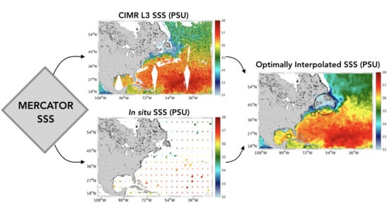
2.2. Processing Chain Description

The CMEMS SSS operational chain combines in situ and satellite-derived observations using the multidimensional OI technique originally introduced by Buongiorno Nardelli 2012 [15] and based on the findings of Bretherton et al. 2016 [16]. Presently, this processing chain provides global L4 weekly SSS mapped over a 1/4${}^{\circ }$ regular grid. The algorithm is based on the assumption that SSS and SST covary at spatial scales smaller than those characterizing atmospheric fluxes. This allows us to extract useful dynamical information from the high-pass filtered satellite L4 SSTs for use with the SSS fields.The L4 SSTs are generally obtained by merging microwave and infrared observations, the latter having resolutions $\mathcal{O}$(1 km) [17]. and provide guidance to the OI system when interpolating SSS fields resulting in an enhanced effective resolution compared to simple space-time interpolation approaches. The technique, originally developed to interpolate in situ SSS, was successively adapted to ingest satellite observations from SMOS and finally calibrated to compute dynamically consistent SSS/SSD datasets [10,11,18]. The theoretical framework of the SSS multivariate OI is briefly illustrated below, referring the reader to [10,11,15,18] for more details.

The optimal SSS analysis (${\overline{\mathrm{SSS}}}_{\mathrm{analysis}}$) is given by a weighted sum of the SSS observations anomalies (${\overline{\mathrm{SSS}}}_{\mathrm{obs}}$) with respect to a first guess background field (${\overline{\mathrm{SSS}}}_{\mathrm{background}}$). The weights provide an unbiased estimate (i.e., it has the same mean as the true field) with the minimum expected estimate error (in a least squares sense):

$${\overline{\mathrm{SSS}}}_{\mathrm{analysis}}={\overline{\mathrm{SSS}}}_{\mathrm{background}}+\mathrm{C}{(\mathrm{R}+\mathrm{C})}^{-1}({\overline{\mathrm{SSS}}}_{\mathrm{obs}}-{\overline{\mathrm{SSS}}}_{\mathrm{background}}).$$

(1)

In Equation (1), C is the background error covariance matrix and R, assumed diagonal, is the observations error covariance matrix (here defined by constant values per each observation type/platform). In the implementation described by [10,11], the background field is provided by an analysis built from in situ observations alone through a classical OI. More recently, in the framework of CMEMS, the background field estimate was modified by computing a first round of space-time OI based on in situ input data relying on a monthly climatology. The structure of the background error covariance matrix, C, is given by Equation (2):

$$\mathrm{C}(\Delta \mathrm{r},\Delta \mathrm{t},\Delta \mathrm{SST})=e^{-{(\Delta \mathrm{r}/\mathrm{L})}^2}{e}^{-{(\Delta \mathrm{t}/\tau )}^2}{e}^{-{(\Delta \mathrm{SST}/\mathrm{T})}^2},$$

(2)

where:

• $\Delta$r, $\Delta$t, and $\Delta$SST respectively indicate the spatial, temporal, and thermal separations;
• L, $\tau$, and T are the spatial, temporal, and thermal decorrelation lengths. Their values have been defined by previous studies [15] and are L = 500 km, $\tau$ =7 days, T = 2.75 K.
• The SST L4 data are high-pass-filtered (cut-off at 1000 km).

This covariance model approximates a multivariate approach that includes both SSS and SST in the state vector used to build the observation matrix (that is then used to estimate the covariance matrix C). In practice, the multivariate covariance model gives more weight to observations found on the same isothermal of the interpolation point compared to observations found at the same spatial and temporal separation but characterized by different SST values. The L4 SSTs, due to their high spatial resolution, accurately describe the thermal signature of the ocean mesoscale features at global scale. Their ingestion in the OI algorithm has already shown to improve L4 SSS effective resolution (e.g., [11]). Moreover, the processing chain relies on a dataset of pseudo in situ SSS observations to overcome the sparseness of avaliable in situ SSS. The pseudo-observations are extracted from the background field (1 every 16 grid boxes) and are used as additional input. In coastal areas (at distances < 200 km from the coast), the pseudo-observations are taken from the climatological background. This strategy guarantees the homogeneity of the L4 SSS spatial resolution in case of prolonged (in time) or extended (in space) input data gaps during the interpolation process.

In the present study, the input data for the OI processing, i.e., the in situ, satellite, pseudo SSS and high resolution L4 SST, are all derived from the MERCATOR numerical simulations (see also Section 2.3). In Equation (1), the constant values included in the observation error covariance matrix R are divided by the signal variance, thus representing the different noise-to-signal levels for each type of input data. These values have been found through dedicated tuning experiments and are 0.5 for the pseudo observations, 0.1 for the synthetic CIMR satellite SSS and 0.05 for the synthetic in situ observations. The mean value used for CIMR may appear too optimistic (only twice the error associated with synthetic in situ) and could be optimized by considering the expected latitudinal dependence of CIMR error. This dependence, however, is not presently handled by the CMEMS processing chain and is thus left to future developments.

2.3. OSSE Description

Selecting one year (2016) of daily SSS data from the CMEMS MERCATOR global operational model, we subsampled the SSS fields in two ways, according to the following purposes:

• the simulation of synthetic in situ SSS observations;
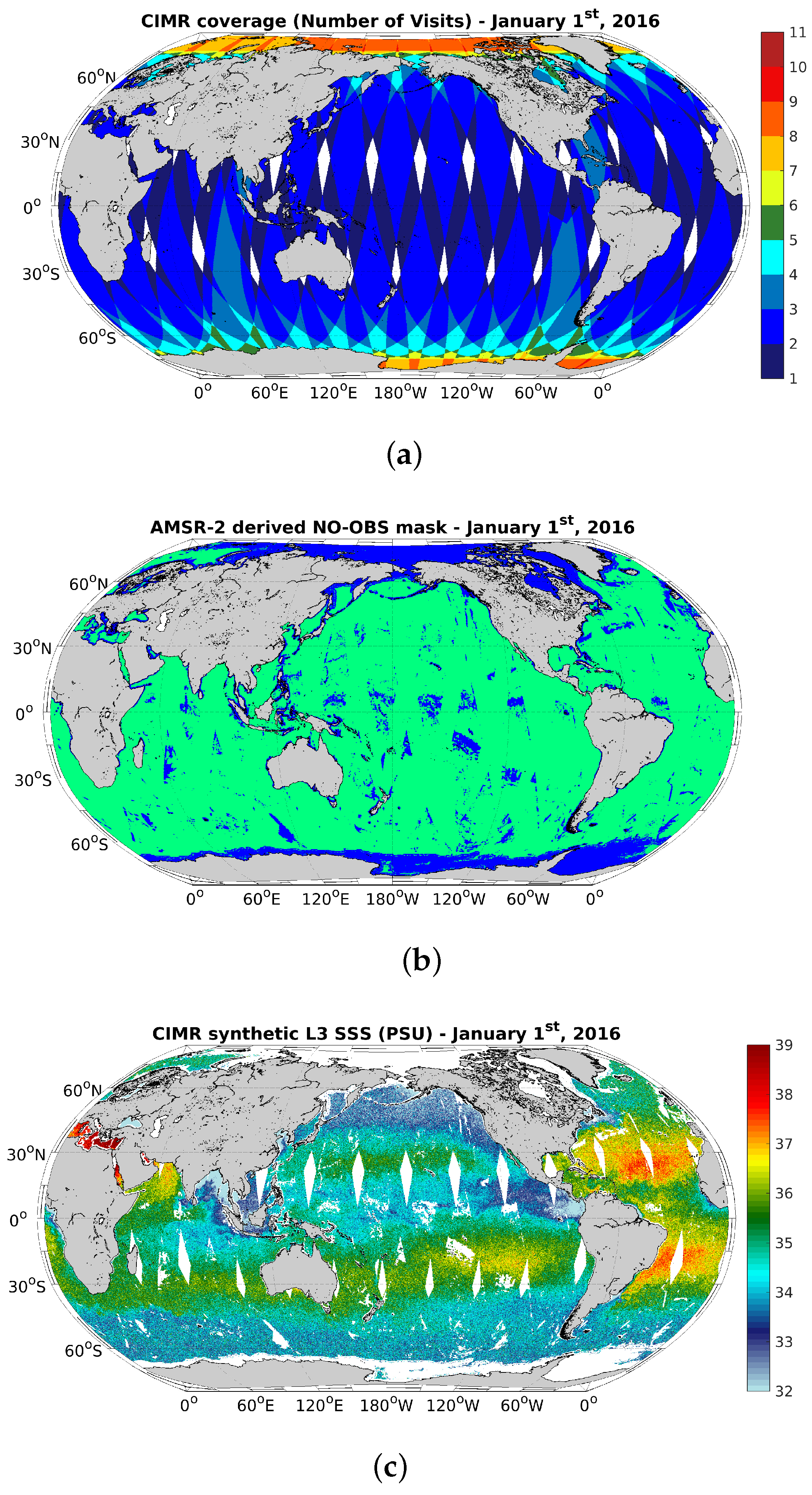
• the simulation of the expected future CIMR satellite observations, taking into account the number of satellite passes over Earth and the expected uncertainty on the SSS retrieval.

The processing chain is run in two different configurations: once ingesting the synthetic in situ SSS alone and, in a second run, the in situ plus the CIMR observations. In both cases, the result of the processing, i.e., the multivariate OI algorithm, is a global map of L4 SSS. Finally, the SSS maps obtained in the two configurations is compared with the original MERCATOR SSS fields, our benchmark. The metrics of the comparison are the root mean square error (RMSE) and the power spectral density (PSD). A flowchart of the OSSE is provided in Figure 1. The details on the simulation of the synthetic data are given in Section 2.4.

2.4. Input Data Preparation: Simulating the SSS Observations

Here, we discuss the generation of the synthetic in situ and CIMR SSS observations.

• We generated synthetic in situ SSS observations from the MERCATOR simulations. This was achieved by colocating the MERCATOR SSS with the quality controlled in situ observations from ARGO floats and CTD casts ingested by the in situ Analysis System (ISAS) [5,6]. Such in situ data were previously binned on daily basis over a regular 1/4${}^{\circ }$ grid. An example of daily in situ SSS is provided in Figure 5b. In the figure, the distribution of the pseudo observations mentioned in Section 2.2 is also given;
• A one year long time series of SSS and SST was extracted from the CMEMS MERCATOR global operational model. In order to mimic the CIMR SSS observations given by the 1.4 GHz measurements (see

  Table 1. CIMR instrument measurement frequencies.

  Frequency (GHz)	Spatial Resolution (Km)
  1.4	55
  6.9	15
  10.65	15
  18.7	5
  36.5	5

  , and [12,19] for the CIMR measurements frequencies), we low-pass filtered the SSSs with a 55 km cut-off wavelength and we remapped them onto a regular 1/4${}^{\circ }$ grid, i.e., exactly the same as the output of the present-day CMEMS SSS L4 processing chain. The more recent release of the CIMR mission requirements document [12] indicates a 1.4 GHz real aperture resolution less than 60 km, which is consistent with the 55 km of [19] also used in the present study. The MERCATOR SSTs were simply remapped over a 1/4${}^{\circ }$ regular grid in order to simulate the L4 SST to be ingested in the SSS OI processing (see Section 2.2).
• We then generate synthetic CIMR-SSS starting from the low-pass filtered MERCATOR SSS described at point 2. This includes both the expected uncertainties on the CIMR SSS and the expected satellite coverage. The SSS retrieval uncertainty (hereinafter referred to as $\sigma$SSS) was provided by the theoretical estimates of Kilic et al. 2018 [19] (see, e.g., Figure 7 in [19]). The authors derived a Look Up Table (LUT) containing the $\sigma$SSS as a function of the local SSS, SST, OWS, TCLW and TCWV. The ranges of variability of the aforementioned parameters are given by

  Table 2. Variability range of the LUT quantities used in [19].

  Variable	Range
  SST (K)	271–303
  OWS (m/s)	0–25
  SSS (PSU)	0–38
  TCWV (kg·m${}^{-2}$)	4–40
  TCLW (g·m${}^{-2}$)	0–500
  $\sigma$SSS (PSU)	0.27–0.99

  .

Based on the LUT estimates, we could generate a time series of daily L4 $\sigma$SSS. This was achieved relying on the daily SST-OWS-TCLW and TCWV observations provided by AMSR-2 [14] plus the daily MERCATOR SSS. In order to fill the gaps in the AMSR-2 observations, we used a linear interpolator, leading to a gap-free proxy of the $\sigma$SSS behaviour. However, in order to rely on higher quality data, the areas relying solely on interpolation were not taken into account when running the OI algorithm. This is further justified at the end of this section and schematically represented in Figure 4 and 5. Checking different SSS-SST-OWS-TCLW-TCWV combinations, we found that the local low SST and high OWS are primarily responsible for the $\sigma$SSS increase, consistently with [19]. An example of the $\sigma$SSS is provided in Figure 2.

Based on these results, we added a white random Gaussian noise to the MERCATOR-SSS according to Equation (3):

$${\mathrm{SSS}}_{\mathrm{noise}}=\mathrm{SSS}+\mathrm{WGN}\left(\sigma \mathrm{SSS}\right),$$

(3)

where $\mathrm{WGN}\left(\sigma \mathrm{SSS}\right)$ stands for a $\sigma$SSS dependent White Gaussian Noise. Figure 3 shows an example of the MERCATOR SSS after addition of the white noise. In the present work, only white noise has been taken into consideration. While actual errors would likely include instruments drift or other variations with time, these effects are still in evaluation [12]. For the moment, the error estimates (as also stated by [19]) are mostly based on the local ocean-atmosphere conditions at the measurement site. The impact of the CIMR radiometric and orbital stability on the global L4 SSS estimates maps is thus left for future investigations.

In order to simulate the CIMR coverage, we used the 28-days cycle of the CIMR satellite overpasses over Earth provided by the European Space Agency, remapped onto a regular 1/4${}^{\circ }$ grid. Such 28 days cycle was applied to our time series of MERCATOR SSS, arbitrarily assuming that the first day corresponds to 1 January 2016 and repeating the cycle throughout the year. The number of overpasses (NVIS) per day is between 0 (in a few small areas of the tropics) and 11 (in polar regions) (Figure 4a). In all the areas where NVIS exceeded 1, we used an averaged SSS obtained as follows: we oversampled the MERCATOR SSS according to NVIS (adding each time a different random Gaussian noise) and then computed the mean SSS in each grid box.

As a final step, in order to make the synthetic satellite-derived SSS more realistic, we derived a sea-ice mask, land mask and rainfall observations mask (i.e., a no observation mask) using the REMSS AMSR-2 SST L3U observations [14]. This is also schematically represented in Figure 4a–c. Except for extreme cases, L-band brightness temperatures are not significantly affected by precipitation, remaining within the CIMR radiometric accuracy [12,20]. In principle, this means a SSS retrieval is possible. However, in these cases, since higher frequency channels are significantly affected by precipitation, the retrieval would require ancillary information on relevant geophysical variables (e.g., SST and OWS). This would require an independent evaluation of the expected uncertainty on the SSS retrieval.

3. Results

In this section, we present the results of the OSSE described in Section 2.3 and summarized by Figure 1. Two different configurations of the CMEMS L4 SSS processing chain (including and not including the CIMR synthetic observations) are qualitatively and quantitatively validated against the MERCATOR SSS, constituting the true SSS field. In the following, the L4 SSS given by the OI of in situ observations and the ones obtained combining in situ plus the CIMR estimates will be referred to as IL4 and CIL4, respectively.

3.1. Qualitative Validation

Observing the IL4 (Figure 5a) and the CIL4 (Figure 5c), a qualitative validation can be carried out using the original MERCATOR SSS as a benchmark (Figure 5e). We present a case study on one of the most dynamically active areas of the global ocean: the Gulf Stream (1 January 2016). In general, when the CIMR observations are not included, the resulting OI SSS misrepresents the salinity values as well as the mesoscale activity found in the benchmark salinity field. Indeed, the IL4 are given by a smooth field, close to a climatological estimate, with mesoscale activity appearing only in proximity of the in situ observations, where the multivariate algorithm can account for the spatial, temporal and thermal decorrelation (given by the L4 SST field) as indicated in Equation (2). This statement is confirmed by visual inspection of Figure 5a–f.

Moreover, in Figure 5, we highlighted the basin south of Newfoundland and New Scotland using a black circle. Here, the IL4 underestimates the true SSS by about 1 to 1.5 PSU. When the CIMR observations are ingested in the OI processing, the salinity values are corrected and agree with the reference SSS. Finally, we discuss the CIMR performances in resolving the signature of two eddies located off New Jersey and in the Gulf of Mexico. In Figure 5a,c,e, these eddies are highlighted by two black squares. If the CIMR observations were not used in the OI processing, their signatures in the SSS field would either disappear or only partially be resolved.

3.2. Quantitative Validation

The potential of the future CIMR SSS is here demonstrated through quantitative analyses. The metrics of the validation are based on the computation of the RMSE and PSD.

3.2.1. Temporal Variability of the CIMR Impact in the CMEMS SSS

We computed the time series of the RMSE between the outputs of the CMEMS L4 processing chain and the true SSS field. Such statistics are based on weekly data for the year 2016. The main results of the validation are summarized by Figure 6a–c. The statistics have been computed in three latitudinal bands: 90${}^{\circ }$S to 45${}^{\circ }$S (referred to as Area S), 45${}^{\circ }$S to 45${}^{\circ }$N (referred to as Area M) and 45${}^{\circ }$N to 90${}^{\circ }$N (referred to as Area N). This choice is due to the behavior of the average $\sigma$SSS, whose map is well approximated by Figure 2, where these areas have been highlighted. The 45${}^{\circ }$S/N latitudes correspond to the areas where the $\sigma$SSS reaches half of its maximum magnitude, i.e., ≃0.45 PSU, and then rapidly increases up to a maximum of ≃0.9 PSU moving towards the polar regions. On the other hand, in the 45${}^{\circ }$S to 45${}^{\circ }$N latitudinal band, the average $\sigma$SSS is mostly around 0.3 PSU.

As a general comment, the quantitative validations of the L4 SSS show that CIMR SSS will undoubtedly bring benefits for the CMEMS SSS operational products. The CIMR SSSs guarantee to reconstruct L4 salinity maps that systematically reduce the RMSE with respect to the true SSS, compared to products relying on in situ observations alone. In the Area M, the RMSE exhibits the largest improvements, whose magnitude is around 50% throughout the whole year 2016. The improvement is evaluated according to Equation (4) [21]:

$$\mathrm{IMPROVE}=100\times \left[1-{\left(\frac{RMS{E}_{CIL4}}{RMS{E}_{IL4}}\right)}^2\right].$$

(4)

In the Area N, the improvements brought by CIMR vary between 20% and 40%, with the largest values observed during summertime. The RMSE time series of both the CIL4 and the IL4 exhibit a seasonal behaviour with enhanced values during summertime (≃3 PSU), which is a known behaviour for the CMEMS SSS, also discussed by Xie et al. 2019 [22]. The Area S is the only region exhibiting slight degradation using CIMR observations within CMEMS. Here, we could observe improvements reaching 30% during the austral Summer and Fall but from June to November, the CIL4 RMSE increases by about 10${}^{-2}$ PSU compared to the IL4 reconstruction, mostly indicating that CIMR is not bringing a useful contribution to the SSS reconstruction in these areas during the austral Spring and Winter.

3.2.2. Spatial Variability of the CIMR Impact in the CMEMS SSS

In order to quantify the spatial variability of the CIMR improvements, we compared the local temporal RMSE between the CIL4 and the IL4. This was achieved by means of Equation (5), using the MERCATOR SSS as a reference:

$$\Delta \mathrm{RMSE}=\mathrm{RMSE}\left({\mathrm{SSS}}^{\mathrm{CIL}4}\right)-\mathrm{RMSE}\left({\mathrm{SSS}}^{\mathrm{IL}4}\right).$$

(5)

The negative $\Delta$RMSE values indicate an RMSE reduction with respect to the true SSS, hence, an improved SSS retrieval given by CIMR. Figure 7a indicates that the CIMR observations improve the SSS retrieval in 63% of the world ocean, exhibiting better performances in the Area M (45${}^{\circ }$S to 45${}^{\circ }$N) and in coastal regions, which are characterized by the main upwelling systems and the larger river inputs. This is easily explained considering that the density of in situ observations is lower in coastal regions than in the open ocean, as confirmed by Figure 7b. In the figure, the white halo located in correspondence of the coastal waters indicates the absence of in situ SSS estimates. Thus, progressively approaching the coastline, the relative contribution of the CIMR observations improve the SSS variability of the L4 interpolated fields. However, the CIMR sensor in itself is not expected to perform better in costal zones (because of a large measurement footprint). This is confirmed by the analyses reported in Figure 8, where both the RMSE${}^{\mathrm{CIL}4}$ and RMSE${}^{\mathrm{IL}4}$ generally increase as the coastline is approached. In the future, provided the characteristics of the receiving antenna, an estimate of the expected land contamination will be possible. This will enable a more realistic evaluation of the CIMR performances within the CMEMS SSS in coastal areas.

An overall CIL4 degradation is observed in the Area S and in the 60${}^{\circ }$W–10${}^{\circ }$W zone of Area N, where the RMSE${}^{\mathrm{CIL}4}$ exceeds the RMSE${}^{\mathrm{IL}4}$ by 0.01 PSU on average, which is also confirmed by Figure 8a,b. This behaviour is discussed in Section 3.3 in more detail. As an additional analysis, we compared the SSS gradients magnitude found in the CIL4 and IL4 reconstructions. This was performed in a similar fashion as for the SSS fields, i.e., computing the $\Delta$RMSE${}_{\nabla }$:

$$\Delta {\mathrm{RMSE}}_{\nabla }=\mathrm{RMSE}\left(\right|\nabla {\mathrm{SSS}}^{\mathrm{CIL}4}\left|\right)-\mathrm{RMSE}\left(\right|\nabla {\mathrm{SSS}}^{\mathrm{IL}4}\left|\right)$$

(6)

with $|\nabla \mathrm{SSS}|=\sqrt{{\left({\partial }_{\mathrm{x}}\mathrm{SSS}\right)}^2+{\left({\partial }_{\mathrm{y}}\mathrm{SSS}\right)}^2}$, where the quantities ${\partial }_x$ and ${\partial }_y$ are estimated via a centered finite differences numerical scheme and the subscripts “x,y” respectively stand for the zonal and meridional directions.

Accurate estimates of the SSS gradients in L4 products is crucial from a physical point of view. Combined with the information on SST, it gives access to the patterns of the surface density gradients, allowing for diagnosing the global ocean surface dynamics. In addition, the surface density gradients allow for predicting the subsurface circulation from surface observations [23], which justifies the interest in evaluating the CIMR contribution for the monitoring of this variable. CIMR itself will provide global SST fields at the same time as SSS based on the use of 6.9 GHz channel data where the real aperture of the CIMR channel is ≃15 km. According to Figure 9, CIMR improves the SSS gradients retrieval in 70% of the world ocean. This is more evident in the Area M and in coastal waters. As for the previous analysis, the Areas S and N show reduced performance, where the averaged $\mathrm{RMSE}\left(\right|\nabla {\mathrm{SSS}}^{\mathrm{CIL}4}\left|\right)$ exceeds by about 0.04 PSU$·{\mathrm{m}}^{-1}$ the one based on in situ observations alone. At latitudes exceeding 75${}^{\circ }$N, the $\Delta {\mathrm{RMSE}}_{\nabla }$ shows alternating patterns of large improvement and degradation. This is not in agreement with the behavior of the $\Delta$RMSE, where an overall improvement of the SSS values is observed. This indicates that, in this region, the CIMR SSS contributes to accurately describe the temporal variability of the SSS but only locally improves the estimate of the SSS gradients with respect to a climatological field.

The statistical significance of the results shown in Figure 7, Figure 8 and Figure 9 was evaluated via a bootstrap resampling technique. The analysis confirmed that both the $\Delta$RMSE and $\Delta$RMSE${}_{\nabla }$ are in the 95% confidence interval.

3.3. Further Insights on the Spatial-Temporal Variability of the CIMR Performances

The spatial-temporal variability of the CIMR performances is consistent with the average physical conditions of the ocean surface throughout the year 2016. The evolution of the daily $\langle \sigma$SSS〉, i.e., the CIMR spatially averaged measurement uncertainty confirms that the Area S exhibits the largest values throughout the year 2016 (Figure 10a). This is mostly due to the persistent low mean SST (≃5 ${}^{\circ }$C) and high OWS (≃10.5 m·s${}^{-1}$) in this area [19] indicating a well mixed surface layer. This was obtained using weekly AMSR-2 observations. Moreover, during the austral Spring and Winter, the $\langle \sigma$SSS〉 exhibits a further increase which results in the degradation of the CIL4 estimates illustrated in Figure 6c.

Following the same logic, the fairly constant CIL4 improvements observed in the Area M are also explained. Indeed, in the 45${}^{\circ }$S to 45${}^{\circ }$N latitudinal band, the $\langle \sigma$SSS〉 is permanently around 0.35, guaranteeing an optimal SSS retrieval from CIMR. The CIMR measurement uncertainty of the Area N enables generally improving the CIL4 estimates compared to the IL4 reconstruction. Here, the $\langle \sigma$SSS〉 also exhibits a larger seasonal cycle than in the Area S, due to the enhanced SST and OWS variability of the northern hemisphere, in agreement with the results of Dunstan et al. 2018 [24]. This explains the time dependence of the CIL4 improvements found in the Area N, yielding a more precise reconstruction during the Summer.

The behaviour of the $\langle \sigma$SSS〉 also explains the spatial variability of the CIMR benefits within the CMEMS SSS operational products, summarized by Figure 7a and Figure 9. These figures suggest that CIMR will improve the SSS and SSS gradients estimates in the 60% and 70% of the world ocean, respectively. Nevertheless, the Area S is the main degradation zone for both the CIL4-SSS and CIL4-SSS spatial gradients. The large values of $\langle \sigma$SSS〉 during April to November 2016 are most likely the responsible of this degradation, whose signature emerges in the $\Delta \mathrm{RMSE}$ and $\Delta {\mathrm{RMSE}}_{\nabla }$.

The present-day version of the CMEMS SSS processing chain may also be responsible for the partial degradation observed in the Area S. In future studies, we plan to further tune of the operational chain in this area. This will be achieved considering a different weighting of the CIMR SSS in the multivariate OI algorithm, given their decreased accuracy during the austral Spring and Winter.

3.4. Spectral Content of IL4 and CIL4

Here, we describe the capability of CIMR to retrieve the signatures of mesoscale activity in the CMEMS SSS. This will be assessed via a spectral analysis of the IL4 and CIL4 compared to the reference SSS provided by MERCATOR. We perform the spectral analyses in five land-free areas of the world ocean: the North and South Atlantic, the North and South Pacific and the Indian Ocean. The SSS power spectral density (PSD) computation is compliant with [11] and is based on Fast Fourier Transform with the Blackman–Harris window for the reduction of spectral leakage.

The spectra are computed over the entire 2016 using weekly data for both the L4 reconstructions. The time average of the mean zonal spectra is presented in Figure 11 as a function of the spatial wavenumber, indicating spectral properties of the IL4, CIL4 and MERCATOR SSS that agree in all the aforementioned investigation areas. Compared to the true SSS, the IL4 spectra (red lines of Figure 11) show a PSD drop around 0.1 degrees${}^{-1}$. On the other hand, the CIMR SSS allows for building interpolated SSS maps with spectral properties that follow the true SSS, except for the addition of noise at scales below 0.8 degrees${}^{-1}$ (on average), where the CIL4 spectra begin to flatten.

The spectral analysis presented here is not fully rigorous from a physical point of view. Indeed, our maps are presented over a regular 1/4${}^{\circ }$ grid and we are computing the spectra over latitudinal extents exceeding 40${}^{\circ }$, thus considering spatial grid separations ranging from approximately 27 to 14 km, e.g., going from the equator up to 60${}^{\circ }$N/S. Nevertheless, the results presented here are still proving that the CIMR SSS are expected to enhance the effective spatial resolution of the CMEMS SSS with respect to reconstructions based on in situ observations. In order to quantify the spectral properties from a physical point of view, we performed the spectral analysis in a 20${}^{\circ }$ box centered over the equator (±10${}^{\circ }$ around the equator) in the Pacific and the Atlantic Oceans, i.e., guaranteeing grid separations around 27 km on average. The behaviour of the spectra are similar to the ones presented in Figure 11. The CIL4 reconstruction spectrum evolves in agreement with the one of the MERCATOR SSS until scales of 1.4 deg${}^{-1}$ where the effect of noise becomes evident. This additional analysis indicates that the CIL4 are dynamically consistent with the MERCATOR fields until scales of approximately 70 km.

4. Discussion and Conclusions

The Copernicus Marine Environment Monitoring Service is presently serving a wide community of users with the distribution, amongst others, of global optimally interpolated L4 SSS (and sea-surface density) mapped on a 1/4${}^{\circ }$ regular grid, updated weekly and based on a combination of in situ, satellite SSS and high-resolution SST data. The CMEMS SSS are obtained combining ARGO and CTD observations with SMOS SSS measurements [10,11,18]. After the SMOS era, the potential availability of the CIMR SSS could guarantee the accuracy and effective spatial resolution of the CMEMS SSS datasets. This was shown throughout this paper via a synthetic CMEMS SSS processing chain relying on simulated CIMR SSS retrievals. The core of our investigation was the CMEMS MERCATOR operational model, which was used to simulate the input SSS for the optimal interpolation processing as well as for assessing the accuracy of the CIMR-based L4 SSS. We focused on the year 2016. The main results of our evaluation study are summarized and discussed here.

CIMR will guarantee the retrieval of improved L4 SSS estimates (CIL4) with respect to optimally interpolated products based on in situ observations alone (IL4). Using the MERCATOR outputs as a benchmark, we obtained that the CIL4 RMSE is systematically reduced throughout the year in the latitudinal band 45${}^{\circ }$S to 90${}^{\circ }$N (Areas M and N), showing improvements up to 50% (based on Equation (4)) compared to the IL4 reconstructions. In the Area S, the CIMR benefits were confirmed during half of the year 2016, exhibiting a slight criticism during the austral Spring and Winter.

In past studies [11], the multivariate algorithm for the production of the L4 SSS was shown to perform much better in the open ocean. Offshore, the high pass filtered SST and SSS are generally more correlated and the assumptions made to derive the multidimensional covariance function are more strictly valid. This is more evident when SSS observations in coastal waters are too sparse, preventing an accurate mapping of the salinity changes related to groundwater fluxes or when the SST patterns are modified by localized heat fluxes (e.g., wind interactions with highly variable coastal orography). In the present study, we showed that the availability of remotely sensed CIMR SSS not only proves useful to monitor salinity changes associated with mesoscale-to-large scale processes in the open ocean, but also significantly improves our capability to describe salinity patterns in coastal areas.

Moreover, the use of the CIMR SSS will enable improving the effective spatial resolution of the global CMEMS L4 SSS, compared to L4 SSS obtained interpolating in situ observations alone. In our OSSE, the CIL4 reconstruction showed spectral properties in agreement with the true SSS, i.e., the MERCATOR model outputs. The optimal interpolation scheme only adds noise to scales smaller than 80 km, according to the tests performed in the Pacific and Atlantic equatorial bands.

These results indicate that the benefits of the potential SSS observations from CIMR will go even beyond the operational requirements within CMEMS. Their application to scientific and societal studies will be wide. The global L4 SSS obtained with CIMR will enable capturing the signatures of the major mesoscale dynamical features, e.g., the main Gulf Stream or Agulhas Rings [25], guaranteeing the monitoring of their spatial distribution and migration pathways. This will contribute to evaluating the global scale SSS distribution and budget. The monitoring of the global SSS is also a key element in studies of water cycle, oceanic water formation and ocean-atmosphere coupled dynamics [26]. For example, Ballabrera-Poy et al. 2002 [27] pointed out that SSS can be crucial in predicting the El Niño Southern Oscillation (ENSO) dynamics over time scales of 6 to 12 months. Indeed, the positive SSS anomalies in proximity of the Pacific equatorial band can modulate ENSO via their impact on the subsurface oceanic stratification. Quite interestingly, CIMR showed optimal measurement performances in the tropical Pacific area. Moreover, the accurate SSS estimate is useful for applications of three-dimensional fields reconstruction from surface information, as pointed out by [7,23,28] for the reconstruction of the three-dimensional horizontal and vertical oceanic motions and tracers. In conclusion, the expected performance of the CIMR mission confirmed the importance of ingesting the CIMR SSS within the framework of the CMEMS SSS data production. The future loss of the SMOS and SMAP missions fully justifies the high priority of the CIMR mission development within the framework of Copernicus.

References

1. Richardson, P.; Bower, A.; Zenk, W. A census of Meddies tracked by floats. Prog. Oceanogr. 2000, 45, 209–250. [Google Scholar] [CrossRef]
2. Bower, A.S.; Hunt, H.D.; Price, J.F. Character and dynamics of the Red Sea and Persian Gulf outflows. J. Geophys. Res. 2000, 105, 6387–6414. [Google Scholar] [CrossRef]
3. Kolodziejczyk, N.; Hernandez, O.; Boutin, J.; Reverdin, G. SMOS salinity in the subtropical North Atlantic salinity maximum: 2. Two-dimensional horizontal thermohaline variability. J. Geophys. Res. Oceans 2015, 120, 972–987. [Google Scholar] [CrossRef] [Green Version]
4. Land, P.E.; Shutler, J.D.; Findlay, H.S.; Girard-Ardhuin, F.; Sabia, R.; Reul, N.; Piolle, J.F.; Chapron, B.; Quilfen, Y.; Salisbury, J.; et al. Salinity from space unlocks satellite-based assessment of ocean Acidification. Environ. Sci. Technol. 2015. [Google Scholar] [CrossRef] [PubMed]
5. Gaillard, F.; Brion, E.; Charraudeau, R. ISAS–V5: Description of the method and user manual. In IFREMER Rapport LPO; LPO: Brest, France, 2009; Volume 9, p. 34. [Google Scholar]
6. Gaillard, F.; Reynaud, T.; Thierry, V.; Kolodziejczyk, N.; Von Schuckmann, K. In situ–based reanalysis of the global ocean temperature and salinity with ISAS: Variability of the heat content and steric height. J. Clim. 2016, 29, 1305–1323. [Google Scholar] [CrossRef]
7. Guinehut, S.; Dhomps, A.L.; Larnicol, G.; Le Traon, P.Y. High resolution 3D temperature and salinity fields derived from in situ and satellite observations. Ocean Sci. 2012, 8, 845–857. [Google Scholar] [CrossRef]
8. Umbert, M.; Hoareau, N.; Turiel, A.; Ballabrera-Poy, J. New blending algorithm to synergize ocean variables: The case of SMOS sea surface salinity maps. Remote Sens. Environ. 2014, 146, 172–187. [Google Scholar] [CrossRef]
9. Olmedo, E.; Taupier-Letage, I.; Turiel, A.; Alvera-Azcárate, A. Improving SMOS Sea Surface Salinity in the Western Mediterranean Sea through Multivariate and Multifractal Analysis. Remote Sens. 2018, 10, 485. [Google Scholar] [CrossRef]
10. Buongiorno Nardelli, B.; Droghei, R.; Santoleri, R. Multi-dimensional interpolation of SMOS sea surface salinity with surface temperature and in situ salinity data. Remote Sens. Environ. 2016, 180, 392–402. [Google Scholar] [CrossRef]
11. Droghei, R.; Buongiorno Nardelli, B.; Santoleri, R. A New Global Sea Surface Salinity and Density Dataset From Multivariate Observations (1993–2016). Front. Mar. Sci. 2018, 5, 84. [Google Scholar] [CrossRef]
12. Donlon, C.J. Copernicus Imaging Microwave Radiometer (CIMR) Mission Requirements Document, Version 2.0; ESA-ESTEC Noordwijk 2201 AZ, The Netherlands; 2019. Available online: http://esamultimedia.esa.int/docs/EarthObservation/Copernicus_CIMR_MRD_v2.0_Issued_20190305.pdf (accessed on 3 August 2019).
13. Nouel, L. Global Ocean 1/12 of a Degree Physics Analysis and Forecast Updated Daily—Product User Manual (CMEMS-GLO-PUM-001-024); Issue 1.4; E.U. Copernicus: Brussels, Belgium, 2019. [Google Scholar]
14. Wentz, F.; Meissner, T.; Gentemann, C.; Hilburn, K.; Scott, J. Remote Sensing Systems GCOM-W1 AMSR2 Daily data, Environmental Suite on 0.25 Degrees Grid, Version V.8 2014. Available online: www.remss.com/missions/amsr (accessed on October 2018).
15. Buongiorno Nardelli, B. A novel approach for the high-resolution interpolation of in situ sea surface salinity. J. Atmos. Ocean. Technol. 2012, 29, 867–879. [Google Scholar] [CrossRef]
16. Bretherton, F.P.; Davis, R.E.; Fandry, C. A technique for objective analysis and design of oceanographic experiments applied to MODE-73. Deep. Sea Res. Oceanogr. Abstr. 1976, 23, 559–582. [Google Scholar] [CrossRef]
17. Robinson, I.S. Measuring the Oceans from Space: The Principles and Methods of Satellite Oceanography; Springer Science & Business Media: Berlin/Heidelberg, Germany, 2004. [Google Scholar]
18. Droghei, R.; Buongiorno Nardelli, B.; Santoleri, R. Combining in situ and satellite observations to retrieve salinity and density at the ocean surface. J. Atmos. Ocean. Technol. 2016, 33, 1211–1223. [Google Scholar] [CrossRef]
19. Kilic, L.; Prigent, C.; Aires, F.; Boutin, J.; Heygster, G.; Tonboe, R.T.; Roquet, H.; Jimenez, C.; Donlon, C. Expected Performances of the Copernicus Imaging Microwave Radiometer (CIMR) for an All-Weather and High Spatial Resolution Estimation of Ocean and Sea Ice Parameters. J. Geophys. Res. Oceans 2018, 123, 7564–7580. [Google Scholar] [CrossRef]
20. Skou, N.; Hoffman-Bang, D. L-band radiometers measuring salinity from space: Atmospheric propagation effects. IEEE Trans. Geosci. Remote Sens. 2005, 43, 2210–2217. [Google Scholar] [CrossRef]
21. Rio, M.H.; Santoleri, R. Improved global surface currents from the merging of altimetry and Sea Surface Temperature data. Remote Sens. Environ. 2018, 216, 770–785. [Google Scholar] [CrossRef]
22. Xie, J.; Raj, R.P.; Bertino, L.; Samuelsen, A.; Wakamatsu, T. Evaluation of Arctic Ocean surface salinities from SMOS and two CMEMS reanalyses against in situ data sets. Ocean Sci. Discuss. 2019. [Google Scholar] [CrossRef]
23. Isern-Fontanet, J.; Lapeyre, G.; Klein, P.; Chapron, B.; Hecht, M. Three-dimensional reconstruction of oceanic mesoscale currents from surface information. J. Geophys. Res. Oceans 2008, 113, 153–169. [Google Scholar] [CrossRef]
24. Dunstan, P.K.; Foster, S.D.; King, E.; Risbey, J.; O’Kane, T.J.; Monselesan, D.; Hobday, A.J.; Hartog, J.R.; Thompson, P.A. Global patterns of change and variation in sea surface temperature and chlorophyll a. Sci. Rep. 2018, 8, 14624. [Google Scholar] [CrossRef]
25. Carton, X. Hydrodynamical Modeling of Oceanic Vortices. Surv. Geophys. 2001, 22, 179–263. [Google Scholar] [CrossRef]
26. Font, J.; Camps, A.; Borges, A.; Martín-Neira, M.; Boutin, J.; Reul, N.; Kerr, Y.H.; Hahne, A.; Mecklenburg, S. SMOS: The challenging sea surface salinity measurement from space. Proc. IEEE 2009, 98, 649–665. [Google Scholar] [CrossRef]
27. Ballabrera-Poy, J.; Murtugudde, R.; Busalacchi, A. On the potential impact of sea surface salinity observations on ENSO predictions. J. Geophys. Res. Oceans 2002, 107, SRF–8. [Google Scholar] [CrossRef]
28. Buongiorno Nardelli, B.; Mulet, S.; Iudicone, D. Three-Dimensional Ageostrophic Motion and Water Mass Subduction in the Southern Ocean. J. Geophys. Res. Oceans 2018, 123, 1533–1562. [Google Scholar] [CrossRef]
Figure 1. Workflow of the observing system simulation experiment.
Remotesensing 11 01818 g001
Figure 2. σ SSS computed according to [19], example from 1 January 2016. The additional information in white are referenced in Section 3.2.1.
Remotesensing 11 01818 g002
Figure 3. (a) MERCATOR SSS, 1 January 2016, Gulf Stream area; (b) MERCATOR SSS with addition of white noise according to Equation (3); 1 January 2016, Gulf Stream area.
Remotesensing 11 01818 g003
Figure 4. Simulating the CIMR observations from the MERCATOR SSS. (a) expected CIMR coverage; (b) daily mask for land, sea-ice and precipitation from AMSR-2 SST observations (blue and green respectively stand for available and unavailable observations); (c) synthetic CIMR observations obtained combining the information on the CIMR overpasses, the AMSR-2 observations and the noise. All of the figures are mapped onto a regular 1/4 grid (the same as the present-day CMEMS L4 SSS) and refer to 1 January 2016.
Remotesensing 11 01818 g004
Figure 5. (a) L4 SSS from in situ observations (IL4); (b) extraction of in situ SSS from the MERCATOR SSS, squares and circles, respectively, stand for pseudo and in situ observations; (c) L4 SSS from the combination of in situ and CIMR observations (CIL4); (d) simulated CIMR L3 SSS; (e) MERCATOR SSS (benchmark); (f) MERCATOR SST. All figures refer to 1 January 2016, in the Gulf Stream Area.
Remotesensing 11 01818 g005
Figure 6. (a) RMSE between the OI L4 SSS and the MERCATOR outputs. Blue and red, respectively, stand for IL4 and CIL4 reconstructions. The statistics are referred to the 45 S to the 45 N latitudinal band (Area M); (b) analyses referred to the the 45 N to the 90 N latitudinal band (Area N); (c) analyses referred to the 90 S to the 45 S latitudinal band (Area S).
Remotesensing 11 01818 g006
Figure 7. (a) Δ RMSE based on weekly data, year 2016; (b) density of in situ SSS for the year 2016. The maximum number of in situ observations is ≃140 (in the North Atlantic). The colorbar is saturated to 5 in order to facilitate the visualization of the measurement sites at a global scale.
Remotesensing 11 01818 g007
Figure 8. (a) RMSE C I L 4 ; (b) RMSE I L 4 .
Remotesensing 11 01818 g008
Figure 9. Δ RMSE based on weekly data, year 2016.
Remotesensing 11 01818 g009
Figure 10. (a) blue line: σ SSS〉 in the 45 S to 45 N latitudinal band (Area M). Red line: σ SSS〉 from 45 N to 90 N (Area N) and from 45 S to 90 S (Area S); (b) same analysis for the AMSR-2 derived OWS; (c) same analysis for the AMSR-2 derived SST.
Remotesensing 11 01818 g010
Figure 11. Time average of the mean zonal spectra of the MERCATOR SSS (green line), the IL4 (red line) and the CIL4 (blue line). The time average is based on weekly data for the year 2016. The spectra are computed in five different areas of the global ocean, referenced in the top panel of the figure.
Remotesensing 11 01818 g011