Detection of Strong NOX Emissions from Fine-scale Reconstruction of the OMI Tropospheric NO2 Product


1
Department of Atmospheric Science, Kongju National University, Gongju 32588, Republic of Korea
2
Air Resources Laboratory, National Oceanic and Atmospheric Administration, College Park, MD 20740, USA
3
Cooperative Institute for Satellite Earth System Studies, University of Maryland, College Park, MD 20740, USA
*
Author to whom correspondence should be addressed.
Remote Sens. 2019, 11(16), 1861; https://doi.org/10.3390/rs11161861
Submission received: 31 May 2019
/
Revised: 1 August 2019
/
Accepted: 7 August 2019
/
Published: 9 August 2019
(This article belongs to the Section Environmental Remote Sensing)
Abstract
:Satellite-retrieved atmospheric NO2 column products have been widely used in assessing bottom-up NOX inventory emissions emitted from large cities, industrial facilities, and power plants. However, the satellite products fail to quantify strong NOX emissions emitted from the sources less than the satellite’s pixel size, with significantly underestimating their emission intensities (smoothing effect). The poor monitoring of the emissions makes it difficult to enforce pollution restriction regulations. This study reconstructs the tropospheric NO2 vertical column density (VCD) of the Ozone Monitoring Instrument (OMI)/Aura (13 × 24 km2 pixel resolution at nadir) over South Korea to a fine-scale product (grid resolution of 3 × 3 km2) using a conservative spatial downscaling method, and investigates the methodological fidelity in quantifying the major Korean area and point sources that are smaller than the satellite’s pixel size. Multiple high-fidelity air quality models of the Weather Research and Forecast-Chemistry (WRF-Chem) and the Weather Research and Forecast/Community Multiscale Air Quality modeling system (WRF/CMAQ) were used to investigate the downscaling uncertainty in a spatial-weight kernel estimate. The analysis results showed that the fine-scale reconstructed OMI NO2 VCD revealed the strong NOX emission sources with increasing the atmospheric NO2 column concentration and enhanced their spatial concentration gradients near the sources, which was accomplished by applying high-resolution modeled spatial-weight kernels to the original OMI NO2 product. The downscaling uncertainty of the reconstructed OMI NO2 product was inherent and estimated by 11.1% ± 10.6% at the whole grid cells over South Korea. The smoothing effect of the original OMI NO2 product was estimated by 31.7% ± 13.1% for the 6 urbanized area sources and 32.2% ± 17.1% for the 13 isolated point sources on an effective spatial resolution that is defined to reduce the downscaling uncertainty. Finally, it was found that the new reconstructed OMI NO2 product had a potential capability in quantifying NOX emission intensities of the isolated strong point sources with a good correlation of R = 0.87, whereas the original OMI NO2 product failed not only to identify the point sources, but also to quantify their emission intensities (R = 0.30). Our findings highlight a potential capability of the fine-scale reconstructed OMI NO2 product in detecting directly strong NOX emissions, and emphasize the inherent methodological uncertainty in interpreting the reconstructed satellite product at a high-resolution grid scale.
1. Introduction
Nitrogen oxides (NOX = NO + NO2) are major criteria pollutants forming photochemical ozone and particulate matters (PM) in the atmosphere, which are emitted from various anthropogenic and biogenic sources such as fossil fuel combustion processes, road traffic exhaust, agricultural fertilizer use, biomass burning, and lightning (e.g., [1,2,3]). The nitrogen oxides and the secondary inorganic aerosols formed from NOX oxidation can impact on human health, ecosystems, and regional radiation budgets [4,5,6]. Park et al. [6] reported that the particulate matters formed by NOX contribute approximately 30.7% in aerosol optical depth (AOD) over East Asia. In Europe, it was shown that the effect of NO2 from urban road traffic on premature mortality was 10 times higher than PM2.5 [7]. As the NOX emitted into the atmosphere rapidly reaches a photochemical equilibrium state given the meteorological and photochemical conditions, the atmospheric concentration measurements of NO2 are used as a proxy of an urbanization level and NOX emission amount (e.g., [8,9,10,11]).
Satellite-based detection of the atmospheric NO2 has been performed for past decades and has been used successfully to reveal anthropogenic and biogenic emission sources: Large cities, industrial complexes, and power plants emissions [12,13,14], agricultural emissions [15,16], lightning emissions [17,18], and wildfire emissions [19,20]. Many researchers have used the atmospheric NO2 column concentration data in assessing the bottom-up anthropogenic emission inventories and in detecting temporal air quality changes in various geographical regions (e.g., [8,9,10,21,22,23]). Kim et al. [9] verified the bottom-up NOX emissions of major urban areas and power plants in the western United States using the atmospheric NO2 column measurements from the Scanning Imaging Absorption Spectrometer for Atmospheric Chartography (SCIAMACHY) and the Ozone Monitoring Instrument (OMI)/Aura products and the regional air quality model of the Weather Research and Forecast-Chemistry (WRF-Chem). In the study, good agreement between the satellite-derived and modeled NO2 columns of power plant emissions implied that the satellite retrievals are feasible to verify the bottom-up anthropogenic emissions monitored continuously in the U.S. Han et al. [21] compared the OMI tropospheric NO2 column data from the Royal Netherlands Meteorological Institute (KNMI) to the Community Multiscale Air Quality modeling system (CMAQ) over the East Asia region in order to evaluate three different bottom-up emission inventories compiled in China, South Korea, and Japan. The study showed a capability of the satellite product in revealing high emission areas over the East Asia region and quantitatively verifying the bottom-up emissions in different seasons on a nationwide scale.
Despite the successful evaluation studies of bottom-up anthropogenic emissions on a coarse resolution (e.g., [24,25,26,27]), the satellite-retrieved NO2 column data have various uncertainty factors associated with the data retrieval processes [9,28,29,30]. In order to improve the OMI NO2 column product, Russell et al. [28] applied a priori NO2 profiles obtained from the WRF-Chem model and high-resolution terrain information. Goldberg et al. [30] used high-resolution a priori NO2 profiles obtained from the CMAQ model along with a spatial downscaling technique, resulting in a better agreement against in-situ NO2 column measurements of the Pandora and Airborne Compact Atmospheric Mapper (ACAM) spectrometers than the original product. The improvement led to an increase of NO2 column densities by 160% in urban areas and a decrease by 20–50% in rural areas compared to the operational NASA OMI product.
Another intrinsic limitation in the satellite products is a spatial smoothing effect caused by its coarse pixel resolution. The ground nadir pixel sizes of operational satellites detecting atmospheric NO2 column abundance are 40 × 320 km2 in the Global Ozone Monitoring Experiment (GOME) instrument on board the second European Remote Sensing satellite (ERS-2) [13], 30 × 60 km2 in the SCIAMACHY instrument on board ENVISAT [12,31], 13 × 24 km2 in the OMI instrument on board the Aura [14], and 40 × 80 km2 in the GOME-2 instrument on board Metop-A1 [32]. Meanwhile, anthropogenic emission sources (e.g., cities, industrial complexes) are generally smaller in size than the satellites’ single pixel, consequently steep gradients in atmospheric NO2 columns are poorly represented near the source regions (spatial smoothing effect) (e.g., [8,33,34]). Heue et al. [33] compared the OMI and SCIAMACHY NO2 column data over an industrial area in South Africa against an airborne NO2 column measurement. The satellites detected spatial enhancement in atmospheric NO2 column concentration over the source region, but failed to represent strong spatial gradients found in the aircraft measurement which showed 4–9 times higher NO2 column densities over the source region than the OMI product.
The spatial smoothing effect embedded in the low-resolution satellite products is a critical barrier in quantifying strong emission sources, especially narrow-isolated sources with a scale of less than a few kilometers. The oversampling approach has been developed and improved in order to enhance spatial and temporal variations of satellite-detected pixel data at finer grid scales [35,36,37,38]. Various gridding algorithms have been applied with different complexities to generate gridded products from satellite-detected orbital signals. The simplest method is based on common spatial interpolation methods such as linear interpolation, spline interpolation, and kriging methods [39]. Meanwhile, the physics-based oversampling approach proposed by Sun et al. [38] is one of the advanced methods, in which a generalized 2-dimensional Gaussian function is used to represent the spatial response function of each pixel detected by a satellite sensor. Many studies have been done based on the gridded products, such as an emission estimate (e.g., [40,41]), an environmental exposure assessment (e.g., [42,43]), and source identification (e.g., [44,45,46]). The oversampling approach is able to generate spatially enhanced satellite products finer than their original pixel resolution by virtue of the temporally averaging multiple pixel data over a target grid, which simultaneously results in decreased temporal resolution. This may be conceptually valid when the concentrations detected by a satellite are assumed to be stationary during the averaging period. Directional composite averaging of chemical plumes following local wind direction in a specific source is a method that can be applied to overcome the limitation [37]. The spatial response function in Sun et al. [38] represents a sensitivity distribution of a satellite’s sub-pixel in terms of the sensor’s detection ability, and the information about spatial concentration distribution of chemical plumes within a satellite pixel is not taken into account, which is an apparent limitation of the oversampling method. On the other hand, Kim et al. [47] proposed a conservative downscaling method to reconstruct the spatial distribution of concentration within a satellite pixel, for which the spatial-weight kernel is calculated from high-resolution spatial concentration data simulated by a high-fidelity air quality model. Unlike the oversampling methods, the method is able to reconstruct the fine-scale spatial distribution of atmospheric concentration on each satellite pixel without the temporal averaging process. Meanwhile, the downscaled products depend on the fidelity of the air quality model applied to calculate the spatial-weight kernels of the satellite pixels, which causes additional downscaling errors in generating the fine-scale satellite products. Recent studies found the conservative downscaling method useful to represent strong spatial gradients over large source areas on a city scale, comparing well with in-situ measurements [27,30,48]. However, the downscaling errors associated with an air quality model are not investigated in those studies which used a single air quality model. This study aims to investigate the methodological fidelity of the conservative spatial downscaling method in quantifying strong NOX emission sources over South Korea and the downscaling uncertainties associated with inclusion of multiple air quality models. To do this, the OMI NO2 column data were reconstructed over South Korea using independent high-fidelity air quality models of WRF-Chem and CMAQ.
The manuscript is structured as follows: Section 2 describes the air quality models, the OMI NO2 columns data, and the conservative spatial downscaling method. Section 3 presents the original and newly reconstructed OMI NO2 products over South Korea. Further discussed are the methodological uncertainty, the smoothing effect, and the potential capability of the reconstructed OMI NO2 product in quantifying the major point sources over South Korea. The summary and conclusions follow in Section 4.
2. Data and Method
2.1. Regional Air Quality Models: WRF-Chem and WRF/CMAQ
The regional air quality models of WRF-Chem [49] and CMAQ [50] were applied to produce high-resolution spatial distribution of NO2 concentration over the South Korean region. The WRF model is a three-dimensional Eulerian meteorological model that solves dynamic/thermodynamic conservation equations of momentum, heat, moisture, and mass, and atmospheric physical processes of radiative transfer, turbulent mixing, surface-atmosphere interaction, and precipitation, thus being capable of simulating multiscale atmospheric phenomena [51]. The WRF-Chem model is an on-line air quality model that includes chemical transformation, source emissions, dry and wet deposition of chemical gaseous and aerosol species within the WRF model. The model simultaneously integrates the meteorological and chemical processes in a model’s integration time step, thus is able to efficiently represent complex interactions among those physical and chemical processes. The CMAQ model is another three-dimensional Eulerian air quality model that has been developed primarily for regional air quality forecasts by the U.S. Environmental Protection Agency (EPA). It calculates the evolution of the atmospheric gaseous and aerosol species through representing meteorological and chemical processes. Meteorological fields are independently prepared for the model, and they are subsequently fed to the CMAQ model through a meteorology-chemistry interface processor (MCIP) package. In this study, the WRF model is used to produce meteorological fields required for running the CMAQ model (WRF/CMAQ). Both the air quality models have been widely applied for various meteorological and environmental problems such as air quality forecasts, emissions evaluations, regulatory applications, and scientific investigations (e.g., [9,52,53,54,55,56,57]).
The WRF-Chem (ver. 3.9.1) and WRF/CMAQ (ver. 3.6.1/ver. 4.7.1) models were configured with three domains to model atmospheric NO2 column concentrations over South Korea (Figure 1). The outermost domain covered a large East Asia region including China, Japan, and South Korea, with a horizontal grid resolution of 27 km (174 × 128 mesh). The second and third nested domains were configured with a horizontal grid resolution of 9 km (69 × 90 mesh) and 3 km (180 × 225 mesh), respectively, covering the whole South Korean region. The vertical grids were stretched ranging from ~16 m above ground level at the lowest grid to ~20 km (50 hPa) at the domain top. The WRF-Chem model simulates both meteorological and chemical species at 35 sigma levels, while the CMAQ model calculates chemical species at 16 reduced sigma levels for computational efficiency. The MCIP produces the reduced meteorological fields compatible to the CMAQ using the WRF-simulated meteorological fields at 35 sigma levels.
The physical options used in the WRF simulations were identically configured with the Goddard scheme [58] and the rapid radiative transfer model (RRTM) [59] for shortwave and longwave radiation, the YSU scheme [60] for atmospheric boundary layer turbulence, the NoahLSM [61] for surface-atmosphere interactions, and the WSM3 scheme [62] and the Kain-Fritsch scheme [63] for grid-scale microphysics and sub-grid convective cloud parameterization. The exceptions were the Dudhia shortwave radiation scheme [64] and the Grell-3D cumulus parameterization in the WRF-Chem. The WRF-Chem uses the regional atmospheric chemistry mechanism (RACM) [65] and the modal aerosol dynamics model for Europe/Secondary organic aerosol model (MADE/SORGAM) [66,67] for gaseous and aerosol chemical mechanisms, respectively, while the WRF/CMAQ uses the Statewide Air Pollution Research Center, Version 99 (SAPRC-99) [68] and the aerosol module version 5 AERO5 [69]. The Model Inter-Comparison Study for Asia 2010 (MICS Asia 2010) developed for the East Asia air quality project [70,71] was used to produce anthropogenic emissions. The MICS-Asia 2010 emissions were gridded compatible to the model domains using the sparse matrix operator kernel for emissions (SMOKE) [72] emission processing module. The chemical speciation of volatile organic compounds (VOCs) follows the SAPRC-99 for WRF/CMAQ and the RACM for the WRF-Chem, and the chemical conversion between the two mechanisms follows Lee et al. [55]. Biogenic emissions were produced by the model of emissions of gases and aerosols from nature, version 2 (MEGAN 2) [73]. Table 1 summarizes the physical and chemical processes used in simulations of the WRF-Chem and the WRF/CMAQ models.
The simulations were carried for first 15 days of each January, April, July, and October (total 60 days) in 2015. The meteorological initial and boundary conditions of the outermost domain were obtained from the National Centers for Environmental Prediction-Final Analysis (NCEP FNL) that is a global reanalysis data with a spatial resolution of 1° × 1° and a temporal resolution of 6 hrs. The simulated meteorological fields for the outermost domain were nudged to the large-scale reanalyzed meteorological fields of air temperature, humidity, and winds using the 4-dimensional data assimilation (4DDA) technique [74]. The simulations of the nested domains were conducted by a one-way nesting approach.
2.2. Satellite Measurement: OMI/Aura tropospheric NO2 Columns
The OMI tropospheric NO2 vertical column densities (VCD) retrieved by the Royal Netherlands Meteorological Institute Dutch-OMI-NO2 version 2.0 (KNMI DOMINO v2.0) algorithm [75] were used. The OMI instrument, onboard the NASA Aura satellite, passed the equator at ~13:45 local standard time (LST) with a cross-track field of view angle of 114°, a swath width of 2600 km, and a nadir pixel size of 13 × 24 km2. The OMI tropospheric NO2 VCD product was made through a series of data processing procedures. The KNMI OMI NO2 slant column densities were calculated by a differential optical absorption spectroscopy (DOAS) technique, from which the tropospheric NO2 column densities were calculated by separating the stratospheric and tropospheric contribution and subsequently by applying the tropospheric air mass factor that was obtained from the global chemical transport model TM4 and the radiative transfer model DAK [75]. The errors estimated during the retrieval procedures were ~0.25 × 10¹⁵ molecules cm-2 in the separation of stratospheric and tropospheric contribution, ~1.0 × 10¹⁵ molecules cm-2 in the application of the air mass factor, and ~0.7×10¹⁵ molecules cm-2 in the spectral fitting process.
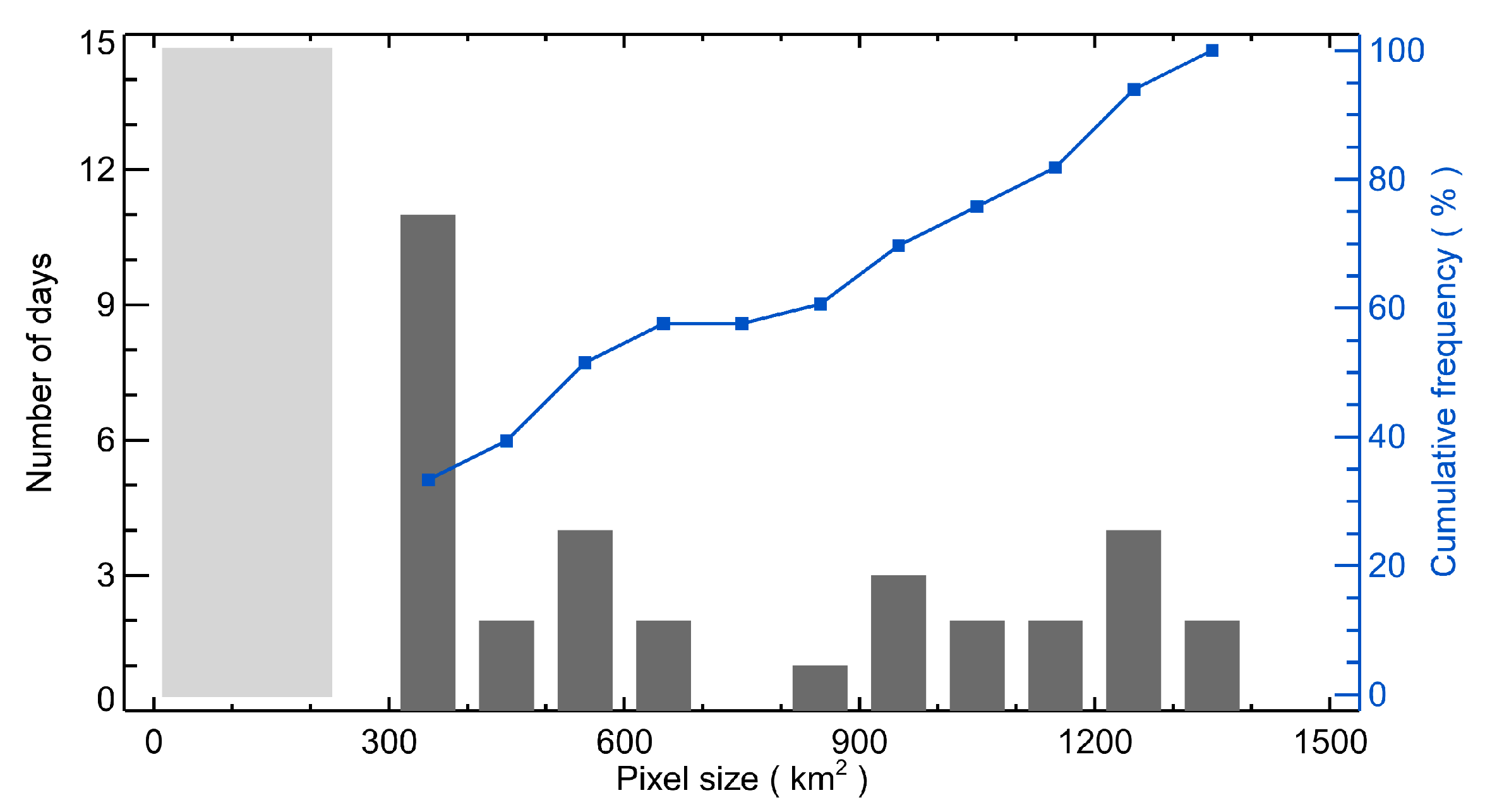
Figure 2 shows the frequency distribution of overpassing days in terms of the mean pixel size of tropospheric NO2 VCD passing over the South Korean region (126°E–130°E; 34°N–8°N). The tropospheric NO2 VCD data were available for 33 days (~55%) before the data quality control among 60 days of the simulation period and the average pixel sizes ranged from 312–1653 km2 in the South Korean region. Approximately 33% of the days had a pixel size close to the satellite’s nadir resolution, while approximately 30% had a mean pixel size of greater than 1000 km2. Meanwhile, the Korean cities have small urbanized areas of ranging from 10.5–227.5 km2 when compared to the satellite pixel sizes, and the spatial sizes of strong point sources such as electric power plants, industrial facilities are much smaller than those of the cities. This indicates that fine-scale spatial distribution of the NOX emissions at a sub-pixel scale should be hardly detected in the OMI NO2 VCD product (shaded in Figure 2).
The quality control procedure was applied to the OMI tropospheric NO2 VCD data because the satellite products were significantly contaminated in the conditions of high cloud fractions and long slant paths. Previous studies generally adopted the filtering conditions of 15–40% for cloud fractions and 1000 km2 for slant path lengths according to the data availability in the area of interest (e.g. [10,21,76,77,78]). This study filtered the NO2 VCD with a cloud fraction of less than 40% and a pixel size of less than 1000 km2 considering frequent cloudy days. Finally, approximately 20% of the OMI NO2 VCD were used in reconstructing the satellite product.
2.3. Conservative Spatial Downscaling Method
The conservative spatial downscaling method proposed by Kim et al. [47] was used, which consists of two-step procedures: Conservative spatial re-gridding and conservative downscaling. The conservative spatial re-gridding procedure is to interpolate the OMI NO2 VCD pixel data to high-resolution air quality model grids by weighting the overlapped areas between the satellite pixel and the model grids. The resulting gridded OMI NO2 VCD data () is calculated as follows:
where is the ith raw OMI NO-2 VCD pixel value, is the area fraction of overlapped on the jth model grid, and is the number of the OMI pixels overlapped on the jth model grid. Each model grid meets . For example, when two OMI NO2 VCD pixels are overlaid on a model grid j, the gridded OMI NO2 VCD is calculated as ()/(). The OMI NO2 VCD is simply re-gridded to the model grids without any changes in spatial distribution.
The conservative downscaling procedure is to calculate the gridded OMI NO2 VCD data () by changing their spatial distribution according to the modeled spatial distribution as follows:
where is a spatial-weight kernel defined by a ratio of modeled NO2 VCD to the OMI NO2 VCD. Here, the spatial-weight kernel was constructed on each ith OMI pixel using high-resolution modeled NO2 VCD in order to conserve the OMI NO2 VCD after applying the spatial-weight kernel. The averaged on the OMI pixel was identical to the OMI NO2 VCD pixel value. In this study, the three-dimensional distribution and evolution of the atmospheric NO2 VCD over South Korea were made by the two independent regional air quality models of the WRF-Chem and WRF/CMAQ so as to produce the spatial-weight kernel . In the modeled NO2 VCD calculation, the KNMI OMI averaging kernel (AK) was applied to the model’s vertical layers of the atmospheric NO2 VCD. It has been known that the averaging kernel is sensitive to the retrieved NO2 VCD [21,78,79].
2.4. Area and Point Sources of NOX Emissions in South Korea
Several major cities and isolated point sources with high NOX emissions over South Korea were selected in order to investigate methodological fidelity of the conservative spatial downscaling method in quantifying the emissions from the sources. The sources were selected based on the annual NOX emissions reported in the South Korean emission inventory data of the Clean Air Policy Support System (CAPPS). Figure 3 shows the spatial distribution of the monthly mean NOX emissions over South Korea along with geographic locations of the major sources. The major Korean cities are denoted by area sources (A), while electric power plants and industrial facilities are denoted by point sources (P) (Figure 3a). The NOX emissions of the area sources were well correlated with the sizes of the urbanized area, while the point sources’ emissions range according to their activities (Figure 3b).
3. Results
3.1. OMI-detected and Modeled NO2 VCD
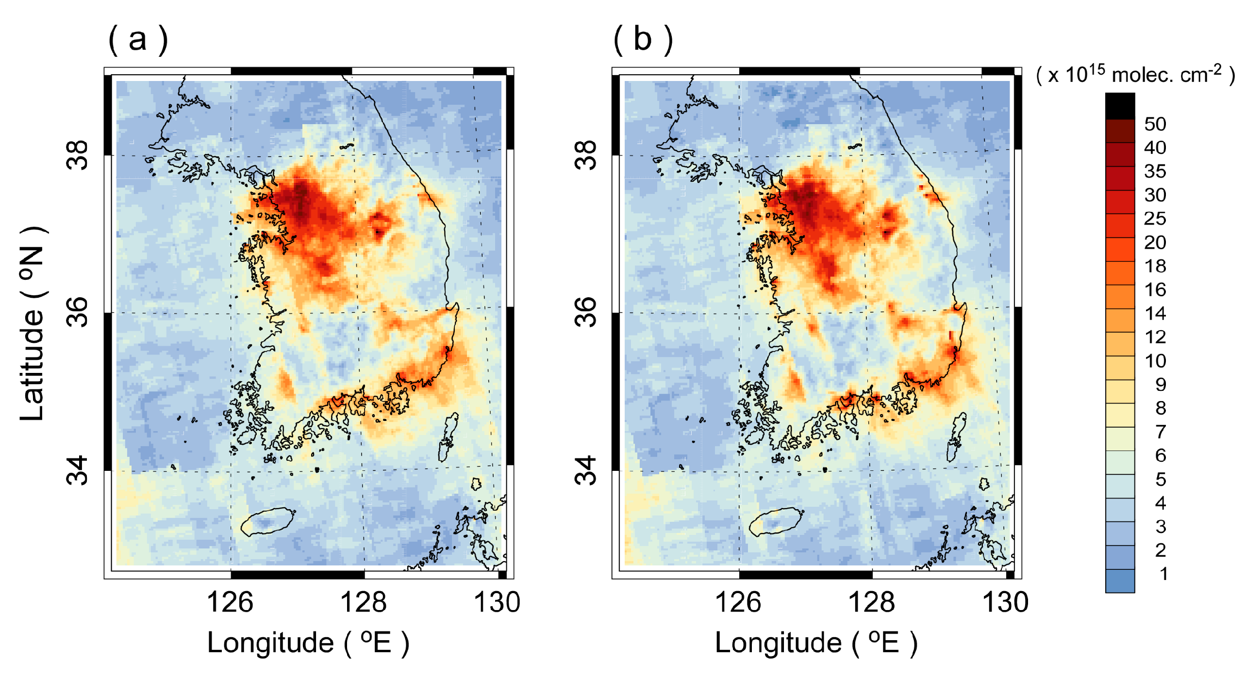
Figure 4 compares the spatial distributions of the re-gridded OMI NO2 VCD and the modeled NO2 VCD by the WRF-Chem and WRF/CMAQ models. The modeled NO2 VCD were averaged for the satellite’s valid pixels applying with the KNMI OMI’s averaging kernels. Large source areas are clearly seen with enhanced concentrations both in the OMI-detected and the modeled NO2 VCD, but distinguishable differences are also apparent. The OMI NO2 VCD is able to discriminate strong NOx emissions from large urbanized areas, but fails to identify strong point emissions (Figure 4a). Previous studies that showed a similar spatial pattern of the KNMI OMI NO2 VCD over the South Korea region at different time periods (e.g., [21,80]) considered the nation-wide spatial average of the OMI NO2 VCD in their analysis. Meanwhile, both the modeled NO2 VCD show more clearly enhanced signals of the strong point sources as well as the urbanized area sources than the OMI NO2 product (Figure 4b,c), which is also spatially well correlated with the distribution of NOX emissions in Figure 3. The two models simulate similarly the spatial distributions over the South Korea, but the NO2 VCD modeled by the WRF-Chem tends to be higher than the WRF/CMAQ.
Figure 5 compares the OMI-detected and modeled NO2 VCD to evaluate the model performance of the WRF-Chem and WRF/CMAQ in simulating the atmospheric NO2 column concentrations over the South Korean region. The monthly mean OMI NO2 VCD was 3.6 × 10¹⁵ molec. cm-2 in July and 9.0 × 10¹⁵ molec. cm-2 in January, with an annual mean value of 6.7 × 10¹⁵ molec. cm-2. Han et al. [21] reported a similar seasonal change of the KNMI OMI NO2 VCD ranging from 3.4–6.7 × 10¹⁵ molec. cm-2 over the South Korean region in 2006. Kim et al. [80] reported approximately 4.0 × 10¹⁵ molec. cm-2 in summer and 7.0 × 10¹⁵ molec. cm-2 in winter 2010 in the KNMI OMI NO2 VCD Level 3 product. Meanwhile, the WRF-Chem model simulated the higher NO2 VCD levels by 50–145% than the WRF/CMAQ model during the periods. The NO2 VCD modeled by the WRF/CMAQ compared better to the satellite-retrieved atmospheric NO2 column concentrations than the WRF-Chem model. This discrepancy may partly be attributed to the deactivation of aqueous chemistry processes and the configuration of higher vertical grid resolution in the WRF-Chem simulation, but both the models’ NO2 VCD values were within the 1-sigma error range of the satellite product. The atmospheric NO2 VCD simulated by the WRF-Chem and WRF/CMAQ models were used to calculate the spatial-weight kernels in the conservative spatial downscaling method.
3.2. Fine-scale Reconstructed OMI NO2 VCD
Figure 6 presents the reconstructed OMI NO2 VCD over the South Korean region by applying the spatial-weight kernels obtained from the independent air quality models. The newly reconstructed OMI NO2 VCD have a spatial resolution of 3 km in accordance with the models’ grid resolution. Figure 7 compares the re-gridded and reconstructed OMI NO2 VCD over a large urbanized area (Seoul metropolitan area) and an area with a few isolated strong point sources. The reconstructed OMI NO2 VCD can reveal the highly urbanized area sources as well as the strong isolated point sources with enhanced spatial gradients and the higher level of column concentrations (Figure 6), which is well compared to the NOX emissions (Figure 3a). In the Seoul metropolitan area, the OMI NO2 VCD downscaled by the WRF-Chem and WRF/CMAQ had values of 3.27 ± 0.75 × 10¹⁶ molec. cm-2 (maximum 4.53 × 10¹⁶ molec. cm-2) and 3.43 ± 0.68×10¹⁶ molec. cm-2 (maximum 4.89 × 10¹⁶ molec. cm-2), respectively, whereas the re-gridded OMI NO2 VCD had relatively low values of 2.63 ± 0.40 × 10¹⁶ molec. cm-2 (maximum of 3.33 × 10¹⁶ molec. cm-2) (Figure 7a–c). During the Megacity Air Pollution Studies-Seoul (MAPS-Seoul) field campaign conducted in May‒June 2015, the atmospheric NO2 VCD detected by the Pandora spectrometer ranged from 1.7‒1.9 Dobson units (DU, 1 DU ≈ 2.7 × 10¹⁶ molec. cm-2) (4.59‒5.13 × 10¹⁶ molec. cm-2) during 12‒14 LST at a site within the Seoul metropolitan area [81]. The fine-scale reconstructed OMI NO2 VCD products compares better to the surface in-situ measurement than the original OMI NO2 VCD. Meanwhile, the capability of the reconstructed OMI NO2 products are apparent in quantifying the emissions from the strong isolated point sources (Figure 7d–f). The strong point sources with a similar amount of NOX emissions were cement industrial facilities separated with a distance of ~20 km. The reconstructed OMI NO2 VCD by the WRF-Chem and WRF/CMAQ had values of 2.23 ± 0.86×10¹⁶ molec. cm-2 (maximum 4.55 × 10¹⁶ molec. cm-2) and 2.13 ± 0.89 × 10¹⁶ molec. cm-2 (maximum 4.35 × 10¹⁶ molec. cm-2), respectively. The signals of the strong point sources were clearly separated in the reconstruct OMI NO2 products, whereas the re-gridded original OMI NO2 product failed to identify the point sources showing relatively lower concentration levels of 1.50 ± 0.12 × 10¹⁶ molec. cm-2 (maximum 1.70 × 10¹⁶ molec. cm-2).
Figure 8 compares the simulated tropospheric NO2 VCD and the reconstructed OMI NO2 VCD by the WRF-Chem and WRF/CMAQ models. The tropospheric NO2 VCD modeled by the WRF-Chem were spatially well correlated with those by the WRF/CMAQ (R = 0.84), but the WRF-Chem model simulated higher NO2 VCD than the WRF/CMAQ (Figure 8a). On the other hand, a better spatial correlation (R = 0.97) was found in the reconstructed OMI NO2 VCD products (Figure 8b). The similarity in the reconstructed OMI products shows that the conservative spatial downscaling method is less sensitive to the concentration level of the modeled NO2 VCD.
The relative differences between the reconstructed OMI NO2 VCD products in Figure 6, Figure 7 and Figure 8 are interpreted as a methodological uncertainty associated with the conservative spatial downscaling method. The downscaling uncertainty is inherent, but has not been quantitatively analyzed in previous studies (e.g., [30,47]). Figure 9 presents the spatial distribution of the reconstructed OMI NO2 VCD averaged by the WRF-Chem and WRF/CMAQ models and the frequency distribution of grid-scale normalized absolute difference (NAD). The NAD is calculated as a downscaling uncertainty metric by . It is clear that the averaged OMI NO2 product reveals highly urbanized areas and strong point sources over the South Korea region (Figure 9a). The downscaling uncertainty in the reconstructed OMI NO2 VCD is relatively large near the strong area and point sources such as cities, industrial complexes, and power plants, resulting from a dissimilar shape of the simulated plumes (Figure 6 and Figure 7). The NAD ranged from 11.1% ± 10.6% (maximum 131.2%) for the whole grid cells and 12.0% ± 11.5% (maximum 108.9%) at the high-concentration grid cells of >8 × 10¹⁵ molec. cm-2. The grid-scale NAD values are less than 10% (20%) at approximately 58% (85%) of the whole grid cells, which is similar in the high-concentration grid cells (Figure 9b). These results indicate that the fine-resolution reconstructed OMI NO2 product has a potential capability in detecting steep concentration gradients found near the strong area and point sources with a reasonable error range compared to the original OMI NO2 VCD (Figure 4a).
3.3. Effective Spatial Resolution and Detection Capability of Strong NOx Emissions
Despite the strong emissions with enhanced spatial gradients and the concentrations being successfully identified in the reconstructed satellite product, the reconstructed OMI NO2 VCD had somewhat large downscaling uncertainty at the grid resolution of 3 km. Therefore, the effective spatial resolution was further investigated by changing an averaging box size near the sources to see how much the downscaling uncertainty reduces. The averaging box sizes of the emission sources increased gradually from 3 × 3 grid cells (9 × 9 km2) to 23 × 23 grid cells (69 × 69 km2). Figure 10a,b compare the re-gridded and the reconstructed OMI NO2 VCD and the associated downscaling uncertainties over the Seoul metropolitan area and an industrial facility site as a function of the averaging box size. For the large urbanized area (Figure 10a), the reconstructed OMI NO2 VCD had higher concentration levels than the re-gridded satellite product by a maximum of 30.0%. The difference between the re-gridded and reconstructed OMI NO2 VCD decreases gradually with an averaging box size until the averaging area is large enough to cover the source region. The downscaling uncertainty in NAD also gradually decreases from ~7% at 225 km2 (15 × 15 km2). For the isolated industrial facility site (Figure 10b), the tropospheric NO2 VCD enhancement in the reconstructed satellite product is apparent by 72.8% at the maximum and decreases rapidly with the averaging area. The estimated NAD is approximately 19% at 9 km2 (3 × 3 km2) as a maximum value, and it decreases rapidly with an averaging box size. The downscaling uncertainty of each area and point sources estimated in NAD are presented for the 6 urbanized area sources and the 13 isolated point sources in Figure 10c,d. The NAD decreases gradually from 17% to 2%, on average, for the urbanized area sources as the averaging area increases, while it decreases more rapidly from 26% to 2% for the isolated point sources. It is also found that the downscaling uncertainty depends on the sources’ characteristics such as the spatial size and distribution of emissions, and the complexities in local meteorology.
The smoothing effect of the original OMI NO2 product in quantifying the atmospheric NO2 column enhancements for the 6 urbanized area and the 13 isolated point sources over South Korea was investigated. A large variability in the downscaling uncertainties of the area and point sources leads to consideration of the effective spatial resolution that is determined by an appropriate averaging box size to reduce the downscaling uncertainties in a reasonable level. The NAD values reduced to less than ~10% for the urbanized area sources when the averaging area was 4–5 times of the source’s aerial size. Meanwhile, the averaging area of 5 × 5 grid cells (15 × 15 km2) for the most isolated point sources led to a significant reduction in NAD ranging within 3–25% except for a few point sources where the downscaling uncertainty still remained as large as 37‒40%. Figure 11 compares the re-gridded and the reconstructed OMI NO2 VCD for the 6 urbanized area sources and the 13 isolated point sources over South Korea on the effective spatial resolution. The reconstructed OMI NO2 VCD were well correlated with the original product for the urbanized area sources (R = 0.99) and the isolated point sources (R = 0.87). However, the reconstructed OMI NO2 VCD were higher by 18‒54% for the urbanized area sources and by 7‒60% for the isolated point sources than the original OMI NO2 product, which is caused by the inability of the satellite’s pixels to resolve the spatial heterogeneity of the sources. In this study, the smoothing effect of the original OMI NO2 product was evaluated by 31.7% ± 13.1% for the urbanized area sources and 32.2% ± 17.1% for the isolated point sources on the effective spatial resolution.
Finally, a potential capability of the reconstructed OMI NO2 product in quantifying the NOX emission intensity for isolated strong point sources was investigated. Figure 12 compares the re-gridded and the reconstructed OMI NO2 VCD of the 13 isolated point sources against the 2015 annual NOX emission of each point source. The NOX emissions are profiled in the Korean national emission inventory database from the direct measurements of stack emissions for the point sources. The reconstructed OMI NO2 VCD were well correlated with the emission intensity of the point sources (R = 0.87), whereas the original OMI product showed only a weakly positive correlation (R = 0.30). The original OMI product shows significant limitations not only in identifying the strong emission sources with a satellite’s sub-pixel scale but also in quantifying the atmospheric NO2 column enhancements corresponding to the emission intensity. In contrast, the newly reconstructed OMI NO2 product shows a great potential capability in quantifying the emissions of the isolated point sources within a reasonable range of downscaling uncertainties.
4. Summary and Conclusions
Large spatial detection coverage of the satellite-retrieved NO2 VCD is beneficial in evaluating air quality models and bottom-up inventory NOX emissions. However, the satellite’s coarse pixel resolution remains a critical limitation in quantifying a strong area and/or point sources and steep gradients on a satellite’s sub-pixel scale. This study reconstructed the KNMI OMI NO2 VCD (13 × 24 km2 at nadir) over South Korea on a spatial resolution of 3 × 3 km2 using a conservative spatial downscaling method to investigate the methodological fidelity in quantifying the atmospheric NO2 column enhancements of the major area and point sources over the South Korean region. Multiple air quality simulations by the WRF-Chem and WRF/CMAQ models were performed over the South Korea region for four different months (60 days) to investigate the downscaling uncertainty in calculating spatial-weight kernels in the conservative spatial downscaling method.
The results showed that the newly reconstructed OMI NO2 VCD based on high-fidelity fine-scale air quality modeling revealed clearly the strong area and point sources with enhanced spatial heterogeneity and steep gradients in accordance with their emission intensities. This is a critical weakness in the original OMI NO2 product that significantly underestimates the atmospheric NO2 column enhancements over the area and point sources. The downscaling uncertainty of the reconstructed OMI NO2 product was estimated by 11.1% ± 10.6% at the whole grid cells over South Korea due to the use of multiple air quality models in the spatial-weight kernel estimate, which is not negligible. The smoothing effect in the original OMI NO2 product was evaluated, on average, by 31.7% ± 13.1% for the 6 urbanized area sources and 32.2% ± 17.1% for the 13 isolated point sources on the effective spatial resolution that is defined by an averaging box size of about 4 times of the urban size and 5 × 5 grid cells (15 × 15 km2) for the area and point sources, respectively. Without considering the geometric smoothing effect, the surface emissions are easily misleading in terms of their intensity and steep spatial gradient. Finally, the potential capability of the reconstructed OMI product was tested in quantifying the isolated strong point sources that are listed in the Korean emission inventory with direct monitored annual NOX emissions. This showed that the isolated strong point sources with different emission intensities are clearly identified in the reconstructed OMI NO2 VCD with a good correlation of 0.87. In contrast, the original OMI NO2 product totally fails to identify the strong point sources and quantify their emission intensities, showing a weakly positive correlation with the emission intensity (R = 0.30).
This study highlights a potential capability of the fine-scale reconstructed OMI NO2 product in quantifying directly strong NOX emissions and their steep spatial gradients and thus in assessing bottom-up inventory emissions for isolated areas and/or point sources that have a spatial scale of less than the satellite’s pixel resolution. It also emphasizes that the methodological uncertainty associated with a spatial-weight kernel estimate should be considered cautiously in interpreting the reconstructed satellite product at a high-resolution grid scale.
The traditional oversampling methods are more beneficial in identifying hidden NOX emissions, but the spatial concentration distribution may be poorly represented due to a relatively coarse spatial and temporal resolution of the product. In contrast, the conservative downscaling method is better in representing fine-scale spatial distribution of identified NOX emissions on a finer spatial and temporal resolution of product. However, the application may be limited to detect unknown sources. Therefore, the oversampling and conservative downscaling methods can be used complementarily.
More research is needed to understand the downscaling uncertainty associated with a priori inventory emissions used in the air quality models, which is another uncertainty factor in the conservative downscaling method. In addition, further validation of the fine-scale reconstructed OMI NO2 product can be useful if high-resolution in-situ measurements and/or remote sensing data are available.
Author Contributions
Conceptualization, S.-H.L.; methodology, J.-H.L., S.-H.L. and H.C.K.; software, J.-H.L. and H.C.K.; investigation, J.-H.L. and S.-H.L.; original draft preparation, J.-H.L. and S.-H.L.
Funding
This work was supported by the National Research Foundation of Korea (NRF) grant funded by the Korea government (MSIT) (No. 2017R1A2B4012975).
Acknowledgments
The authors are grateful to five anonymous reviewers for valuable comments.
Conflicts of Interest
The authors declare no conflict of interest.
References
- Parashar, D.C.; Kulshrestha, U.C.; Sharma, C. Anthropogenic emissions of NOX, NH3 and N2O in India. Nutr. Cycl. Agroecosyst. 1998, 52, 255–259. [Google Scholar] [CrossRef]
- Zhang, R.; Tie, X.; Bond, D.W. Impacts of anthropogenic and natural NOX sources over the U.S. on tropospheric chemistry. Proc. Natl. Acad. Sci. USA 2003, 100, 1505–1509. [Google Scholar] [CrossRef] [PubMed]
- Elliott, E.M.; Kendall, C.; Wankel, S.D.; Burns, D.A.; Boyer, E.W.; Harlin, K.; Bain, D.J.; Butler, T.J. Nitrogen isotopes as indicators of NOX sources contributions to atmospheric deposition across the Midwestern and Northeastern United States. Environ. Sci. Technol. 2007, 41, 7661–7667. [Google Scholar] [CrossRef] [PubMed]
- Fuglestvedt, J.S.; Isaksen, I.S.A.; Wang, W.-C. Estimates of indirect global warming potentials for CH4, CO and NOX. Clim. Chang. 1996, 34, 405–437. [Google Scholar] [CrossRef]
- Wild, O.; Prather, M.J.; Akimoto, H. Indirect long-term global radiative cooling from NOX emissions. Geophys. Res. Lett. 2001, 28, 1719–1722. [Google Scholar] [CrossRef]
- Park, R.S.; Lee, S.; Shin, S.-K.; Song, C.H. Contribution of ammonium nitrate to aerosol optical depth and direct radiative forcing by aerosols over East Asia. Atmos. Chem. Phys. 2014, 14, 2185–2201. [Google Scholar] [CrossRef] [Green Version]
- Harrison, R.M.; Beddows, D.C. Efficacy of recent emissions controls on road vehicles in Europe and implications for public health. Sci. Rep. 2017, 7, 1152. [Google Scholar] [CrossRef] [PubMed]
- Richter, A.; Burrows, J.P.; Nusz, H.; Granier, C.; Niemeier, U. Increase in tropospheric nitrogen dioxide over China observed from space. Nature 2005, 437, 129–132. [Google Scholar] [CrossRef]
- Kim, S.-W.; Heckel, A.; Frost, G.J.; Richter, A.; Gleason, J.; Burrows, J.P.; McKeen, S.; Hsie, E.-Y.; Granier, C.; Trainer, M. NO2 columns in the western United States observed from space and simulated by a regional chemistry model and their implications for NOX emissions. J. Geophys. Res. 2009, 114, D11301. [Google Scholar] [CrossRef]
- Kim, S.-W.; McKeen, S.A.; Frost, G.J.; Lee, S.-H.; Trainer, M.; Richter, A.; Angevine, W.M.; Atlas, E.; Bianco, L.; Boersma, K.F.; et al. Evaluations of NOX and highly reactive VOC emission inventories in Texas and their implications for ozone plume simulations during the Texas Air Quality Study 2006. Atmos. Chem. Phys. 2011, 11, 11361–11386. [Google Scholar] [CrossRef]
- Lee, H.-J.; Kim, S.-W.; Brioude, J.; Cooper, O.R.; Frost, G.J.; Kim, C.-H.; Park, R.J.; Trainer, M.; Woo, J.-H. Transport of NOX in East Asia identified by satellite and in situ measurements and Lagrangian particle dispersion model simulations. J. Geophys. Res. Atmos. 2014, 119, 2574–2596. [Google Scholar] [CrossRef]
- Burrows, J.P.; Hölzle, E.; Goede, A.P.H.; Visser, H.; Fricke, W. SCIAMACHY―Scanning imaging absorption spectrometer for atmospheric chartography. Acta Astronaut. 1995, 35, 445–451. [Google Scholar] [CrossRef]
- Burrows, J.P.; Weber, M.; Buchwitz, M.; Rozanov, V.; Ladstätter-Weißenmayer, A.; Richter, A.; DeBeek, R.; Hoogen, R.; Bramstedt, K.; Eichmann, K.-U.; et al. The Global Ozone Monitoring Experiment (GOME): Mission concept and first scientific results. J. Atmos. Sci. 1999, 56, 151–175. [Google Scholar] [CrossRef]
- Levelt, P.F.; Van den Oord, G.H.J.; Dobber, M.R.; Mälkki, A.; Visser, H.; de Vries, J.; Stammes, P.; Lundell, J.O.V.; Saari, H. The Ozone Monitoring Instrument. IEEE Trans. Geosci. Remote Sens. 2006, 44, 1093–1101. [Google Scholar] [CrossRef]
- Bertram, T.H.; Heckel, A.; Richter, A.; Burrows, J.P.; Cohen, R.C. Satellite measurements of daily variations in soil NOX emissions. Geophys. Res. Lett. 2005, 32, L24812. [Google Scholar] [CrossRef]
- Hudman, R.C.; Russell, A.R.; Valin, L.C.; Cohen, R.C. Interannual variability in soil nitric oxide emissions over the United States as viewed from space. Atmos. Chem. Phys. 2010, 10, 9943–9952. [Google Scholar] [CrossRef] [Green Version]
- Martin, R.V.; Sauvage, B.; Folkins, I.; Sioris, C.E.; Boone, C.; Bernath, P.; Ziemke, J. Space-based constraints on the production of nitric oxide by lightning. J. Geophys. Res. 2007, 112, D09309. [Google Scholar] [CrossRef]
- Bucsela, E.J.; Pickering, K.E.; Huntemann, T.L.; Cohen, R.C.; Perring, A.; Gleason, J.F.; Blakeslee, R.J.; Albrecht, R.I.; Holzworth, R.; Cipriani, J.P.; et al. Lightning-generated NOX seen by the Ozone Monitoring Instrument during NASA’s Tropical Composition, Cloud and Climate Coupling Experiment (TC4). J. Geophys. Res. 2010, 115, D00J10. [Google Scholar] [CrossRef]
- Mebust, A.K.; Russell, A.R.; Hudman, R.C.; Valin, L.C.; Cohen, R.C. Characterization of wildfire NOX emissions using MODIS fire radiative power and OMI tropospheric NO2 columns. Atmos. Chem. Phys. 2011, 11, 5839–5851. [Google Scholar] [CrossRef]
- Schreier, S.F.; Richter, A.; Kaiser, J.W.; Burrows, J.P. The empirical relationship between satellite-derived tropospheric NO2 and fire radiative power and possible implications for fire emission rates of NOX. Atmos. Chem. Phys. 2014, 14, 2447–2466. [Google Scholar] [CrossRef]
- Han, K.M.; Lee, S.; Chang, L.S.; Song, C.H. A comparison study between CMAQ-simulated and OMI-retrieved NO2 columns over East Asia for evaluation of NOX emission fluxes of INTEX-B, CAPSS, and REAS inventories. Atmos. Chem. Phys. 2015, 15, 1913–1938. [Google Scholar] [CrossRef]
- Duncan, B.N.; Lamsal, L.N.; Thompson, A.M.; Yoshida, Y.; Lu, Z.; Streets, D.G.; Hurwitz, M.M.; Pickering, K.E. A space-based, high-resolution view of notable changes in urban NOX pollution around the world (2005-2014). J. Geophys. Res. Atmos. 2016, 121, 976–996. [Google Scholar] [CrossRef]
- Krotkov, N.A.; McLinden, C.A.; Li, C.; Lamsal, L.N.; Celarier, E.A.; Marchenko, S.V.; Swartz, W.H.; Bucsela, E.J.; Joiner, J.; Duncan, B.N.; et al. Aura OMI observations of regional SO2 and NO2 pollution changes from 2005 to 2015. Atmos. Chem. Phys. 2016, 16, 4605–4629. [Google Scholar] [CrossRef]
- Kim, N.K.; Kim, Y.P.; Morino, Y.; Kurokawa, J.; Ohara, T. Verification of NOX emission inventory over South Korea using sectoral activity data and satellite observation of NO2 vertical column densities. Atmos. Environ. 2013, 77, 496–508. [Google Scholar] [CrossRef]
- Tang, W.; Cohan, D.S.; Lamsal, L.N.; Xiao, X.; Zhou, W. Inverse modeling of Texas NOX emissions using space-based and ground-based NO2 observations. Atmos. Chem. Phys. 2013, 13, 11005–11018. [Google Scholar] [CrossRef]
- Kemball-Cook, S.; Yarwood, G.; Johnson, J.; Dornblaser, B.; Estes, M. Evaluating NOX emission inventories for regulatory air quality modeling using satellite and air quality model data. Atmos. Environ. 2015, 117, 1–8. [Google Scholar] [CrossRef]
- Goldberg, D.L.; Saide, P.E.; Lamsal, L.N.; de Foy, B.; Lu, Z.; Woo, J.-H.; Kim, Y.; Kim, J.; Gao, M.; Carmichael, G.; et al. A top-down assessment using OMI NO2 suggests an underestimate in the NOX emissions inventory in Seoul, South Korea, during KOURS-AQ. Atmos. Chem. Phys. 2019, 19, 1801–1818. [Google Scholar] [CrossRef]
- Russell, A.R.; Perring, A.E.; Valin, L.C.; Bucsela, E.J.; Browne, E.C.; Min, K.-E.; Wooldridge, P.J.; Cohen, R.C. A high spatial resolution retrieval of NO2 column densities from OMI: Method and evaluation. Atmos. Chem. Phys. 2011, 11, 8543–8554. [Google Scholar] [CrossRef]
- Laughner, J.L.; Zare, A.; Cohen, R.C. Effects of daily meteorology on the interpretation of space-based remote sensing of NO2. Atmos. Chem. Phys. 2016, 16, 15247–15264. [Google Scholar] [CrossRef]
- Goldberg, D.L.; Lamsal, L.N.; Loughner, C.P.; Swartz, W.H.; Lu, Z.; Streets, D.G. A high-resolution and observationally constrained OMI NO2 satellite retrieval. Atmos. Chem. Phys. 2017, 17, 11403–11421. [Google Scholar] [CrossRef]
- Bovensmann, H.; Burrows, J.P.; Noël, F.S.; Rozanov, V.V. SCIAMACHY: Mission objectives and measurement modes. J. Atmos. Sci. 1999, 56, 127–150. [Google Scholar] [CrossRef]
- Callies, J.; Corpaccioli, E.; Eisinger, M.; Hahne, A.; Lefebvre, A. GOME-2-Metop’s second-generation sensor for operational ozone monitoring. ESA Bull. 2000, 102, 28–36. [Google Scholar]
- Heue, K.-P.; Wagner, T.; Broccardo, S.P.; Walter, D.; Piketh, S.J.; Ross, K.E.; Beirle, S.; Platt, U. Direct observation of two dimensional trace gas distributions with an airborne Imaging DOAS instrument. Atmos. Chem. Phys. 2008, 8, 6707–6717. [Google Scholar] [CrossRef] [Green Version]
- Hilboll, A.; Richter, A.; Burrows, J.P. Long-term changes of tropospheric NO2 over megacities derived from multiple satellite instruments. Atmos. Chem. Phys. 2013, 13, 4145–4169. [Google Scholar] [CrossRef]
- de Foy, B.; Krotkov, N.A.; Bei, N.; Herndon, S.C.; Huey, L.G.; Martinez, A.-P.; Ruiz-Suárez, L.G.; Wood, E.C.; Zavala, M.; Molina, L.T. Hit from both sides: Tracking industrial and volcanic plumes in Mexico City with surface measurements and OMI SO2 retrievals during the MILAGRO field campaign. Atmos. Chem. Phys. 2009, 9, 9599–9617. [Google Scholar] [CrossRef]
- Russell, A.R.; Valin, L.C.; Bucsela, E.J.; Wenig, M.O.; Cohen, R.C. Space-based constraints on spatial and temporal patterns of NOx emission in California, 2005–2008. Environ. Sci. Technol. 2010, 44, 3608–3615. [Google Scholar] [CrossRef] [PubMed]
- Lu, Z.; Streets, D.G.; de Foy, B.; Lamsal, L.N.; Duncan, B.N.; Xing, J. Emissions of nitrogen oxides from US urban areas: Estimation from Ozone Monitoring Instrument retrievals for 2005–2014. Atmos. Chem. Phys. 2015, 15, 10367–10383. [Google Scholar] [CrossRef]
- Sun, K.; Zhu, L.; Cady-Pereira, K.; Miller, C.C.; Chance, K.; Clarisse, L.; Coheur, P.-F.; Abad, G.G.; Huang, G.; Liu, X.; et al. A physics-based approach to oversample multi-satellite, multispecies observations to a common grid. Atmos. Meas. Tech. 2018, 11, 6679–6701. [Google Scholar] [CrossRef] [Green Version]
- Li, J.; Heap, A.D. Spatial interpolation methods applied in the environmental sciences: A review. Environ. Model. Softw. 2014, 53, 173–189. [Google Scholar] [CrossRef]
- Beirle, S.; Boersma, K.F.; Platt, U.; Lawrence, M.G.; Wagner, T. Megacity emissions and lifetimes of nitrogen oxides probed from space. Science 2011, 333, 1737–1739. [Google Scholar] [CrossRef]
- Zhu, L.; Jacob, D.J.; Mickley, L.J.; Marais, E.A.; Cohan, D.S.; Yoshida, Y.; Duncan, B.N.; Abad, G.G.; Chance, K.V. Anthropogenic emissions of highly reactive volatile organic compounds in eastern Texas inferred from oversampling of satellite (OMI) measurements of HCHO columns. Environ. Res. Lett. 2014, 9, 114004. [Google Scholar] [CrossRef] [Green Version]
- Geddes, J.A.; Martin, R.V.; Boys, B.L.; van Donkelaar, A. Long-term trends worldwide in ambient NO2 concentrations inferred from satellite observations. Environ. Health Perspect. 2016, 124, 281–289. [Google Scholar] [CrossRef] [PubMed]
- Zhu, L.; Jacob, D.J.; Keutsch, F.N.; Mickley, L.J.; Scheffe, R.; Strum, M.; Abad, G.G.; Chance, K.; Yang, K.; Rappenglück, B.; et al. Formaldehyde (HCHO) as a hazardous air pollutant: Mapping surface air concentrations from satellite and inferring cancer risks in the United States. Environ. Sci. Technol. 2017, 51, 5650–5657. [Google Scholar] [CrossRef] [PubMed]
- McLinden, C.A.; Fioletov, V.; Boersma, K.F.; Krotkov, N.; Sioris, C.E.; Veefkind, J.P.; Yang, K. Air quality over the Canadian oil sands: A first assessment using satellite observations. Geophys. Res. Lett. 2012, 39, L04804. [Google Scholar] [CrossRef]
- McLinden, C.A.; Fioletov, V.; Shephard, M.W.; Krotkov, N.; Li, C.; Martin, R.V.; Moran, M.D.; Joiner, J. Space-based detection of missing sulfur dioxide sources of global air pollution. Nat. Geosci. 2016, 9, 496–500. [Google Scholar] [CrossRef]
- Kort, E.A.; Frankenberg, C.; Costigan, K.R.; Lindenmaier, R.; Dubey, M.K.; Wunch, D. Four corners: The largest US methane anomaly viewed from space. Geophys. Res. Lett. 2014, 41, 6898–6903. [Google Scholar] [CrossRef]
- Kim, H.C.; Lee, P.; Judd, L.; Pan, L.; Lefer, B. OMI NO2 column densities over North American urban cities: The effect of satellite footprint resolution. Geosci. Model Dev. 2016, 9, 1111–1123. [Google Scholar] [CrossRef]
- Kim, H.C.; Lee, S.-M.; Chai, T.; Ngan, F.; Pan, L.; Lee, P. A conservative downscaling of satellite-detected chemical compositions: NO2 column densities of OMI, GOME-2, and CMAQ. Remote Sens. 2018, 10, 1001. [Google Scholar] [CrossRef]
- Grell, G.A.; Peckham, S.E.; Schmitz, R.; McKeen, S.A.; Frost, G.; Skamarock, W.C.; Eder, B. Fully coupled “online” chemistry within the WRF model. Atmos. Environ. 2005, 39, 6957–6975. [Google Scholar] [CrossRef]
- Byun, D.; Schere, K.L. Review of the governing equations, computational algorithms, and other components of the Models-3 Community Multiscale Air Quality (CMAQ) modeling system. Appl. Mech. Rev. 2006, 59, 51–77. [Google Scholar] [CrossRef]
- Skamarock, W.C.; Klemp, J.B. A time-split nonhydrostatic atmospheric model for weather research and forecasting applications. J. Comput. Phys. 2008, 227, 3465–3485. [Google Scholar] [CrossRef]
- Lee, S.-H.; Kim, S.-W.; Trainer, M.; Frost, G.J.; McKeen, S.A.; Cooper, O.R.; Flocke, F.; Holloway, J.S.; Neuman, J.A.; Ryerson, T.; et al. Modeling ozone plumes observed downwind of New York city over the North Atlantic ocean during the ICARTT field campaign. Atmos. Chem. Phys. 2011, 11, 7375–7397. [Google Scholar] [CrossRef]
- Tuccella, P.; Curci, G.; Visconti, G.; Bessagnet, B.; Menut, L.; Park, R.J. Modeling of gas and aerosol with WRF/Chem over Europe: Evaluation and sensitivity study. J. Geophys. Res. 2012, 117, D3303. [Google Scholar] [CrossRef]
- Han, K.M.; Song, C.H. A budget analysis of NOX column losses over the Korean peninsula. Asia Pac. J. Atmos. Sci. 2012, 48, 55–65. [Google Scholar] [CrossRef]
- Lee, J.-H.; Chang, L.-S.; Lee, S.-H. Simulation of air quality over South Korea using the WRF-Chem model: Impacts of chemical initial and lateral boundary conditions. Atmosphere 2015, 25, 639–657. (In English) [Google Scholar] [CrossRef]
- Tong, D.Q.; Lamsal, L.; Pan, L.; Ding, C.; Kim, H.; Lee, P.; Chai, T.; Pickering, K.E.; Stajner, I. Long-term NOX trends over large cities in the United States during the great recession: Comparison of satellite retrievals, ground observations, and emission inventories. Atmos. Environ. 2015, 107, 70–84. [Google Scholar] [CrossRef]
- Zhang, Y.; Zhang, X.; Wang, L.; Zhang, Q.; Duan, F.; He, K. Application of WRF/Chem over East Asia: Part, I. Model evaluation and intercomparison with MM5/CMAQ. Atmos. Environ. 2016, 124, 285–300. [Google Scholar] [CrossRef]
- Chou, M.-D.; Suarez, M.J.; Ho, C.-H.; Yan, M.M.-H.; Lee, K.-T. Parameterizations for cloud overlapping and shortwave single-scattering properties for use in general circulation and cloud ensemble models. J. Clim. 1998, 11, 201–214. [Google Scholar] [CrossRef]
- Mlawer, E.J.; Taubman, S.J.; Brown, P.D.; Iacono, M.J.; Clough, S.A. Radiative transfer for inhomogeneous atmospheres: RRTM, a validated correlated-k model for the longwave. J. Geophys. Res. 1997, 102, 16663–16682. [Google Scholar] [CrossRef] [Green Version]
- Hong, S.-Y.; Noh, Y.; Dudhia, J. A new vertical diffusion package with an explicit treatment of entrainment processes. Mon. Weather Rev. 2006, 134, 2318–2341. [Google Scholar] [CrossRef]
- Chen, F.; Dudhia, J. Coupling an advanced land surface-hydrology model with the Penn State-NCAR MM5 modeling system. Part I: Model implementation and sensitivity. Mon. Weather Rev. 2001, 129, 569–585. [Google Scholar] [CrossRef]
- Hong, S.-Y.; Dudhia, J.; Chen, S.H. A revised approach to ice microphysical processes for the bulk parameterization of clouds and precipitation. Mon. Weather Rev. 2004, 132, 103–120. [Google Scholar] [CrossRef]
- Kain, J.S. The Kain—Fritsch convective parameterization: An update. J. Appl. J. Appl. Meteorol. 2004, 43, 170–181. [Google Scholar] [CrossRef]
- Dudhia, J. Numerical study of convection observed during the winter monsoon experiment using a mesoscale two-dimensional model. J. Atmos. Sci. 1989, 46, 3077–3107. [Google Scholar] [CrossRef]
- Stockwell, W.R.; Kirchner, F.; Kuhn, M.; Seefeld, S. A new mechanism for regional atmospheric chemistry modeling. J. Geophys. Res. 1997, 102, 25847–25879. [Google Scholar] [CrossRef] [Green Version]
- Ackermann, I.J.; Hass, H.; Memmesheimer, M.; Ebel, A.; Binkowski, F.S.; Shankar, U. Modal aerosol dynamics model for Europe: Development and first applications. Atmos. Environ. 1998, 32, 2981–2999. [Google Scholar] [CrossRef]
- Schell, B.; Ackermann, I.J.; Hass, H.; Binkowski, F.S.; Ebel, A. Modeling the formation of secondary organic aerosol within a comprehensive air quality model system. J. Geophys. Res. 2001, 106, 28275–28293. [Google Scholar] [CrossRef]
- Cater, W.P.L. Documentation of the SAPRC-99 chemical mechanism for VOC reactivity assessment. In Final Report to the California Air Resources Board; Available online: https://intra.engr.ucr.edu/~carter/pubs/s99doc.pdf (accessed on 5 May 2019).
- Foley, K.M.; Roselle, S.J.; Appel, K.W.; Bhave, P.V.; Pleim, J.E.; Otte, T.L.; Mathur, R.; Sarwar, G.; Young, J.O.; Gilliam, R.C.; et al. Incremental testing of the Community Multiscale Air Quality (CMAQ) modeling system version 4.7. Geosci. Model Dev. 2010, 3, 205–226. [Google Scholar] [CrossRef] [Green Version]
- Carmichael, G.R.; Calori, G.; Hayami, H.; Uno, I.; Cho, S.-Y.; Engardt, M.; Kim, S.-B.; Ichikawa, Y.; Ikeda, Y.; Woo, J.-H.; et al. The MICS-Asia study: Model intercomparison of long-range transport and sulfur deposition in East Asia. Atmos. Environ. 2002, 36, 175–199. [Google Scholar] [CrossRef]
- Li, M.; Zhang, Q.; Kurokawa, J.-I.; Woo, J.-H.; He, K.; Lu, Z.; Ohara, T.; Song, Y.; Streets, D.G.; Carmichael, G.R.; et al. MIX: A mosaic Asian anthropogenic emission inventory under the international collaboration framework of the MICS-Asia and HTAP. Atmos. Chem. Phys. 2017, 17, 935–963. [Google Scholar] [CrossRef]
- Benjey, W.; Houyoux, M.; Susick, J. Implementation of the SMOKE emission data processor and SMOKE tool input data processor in models-3. U.S. EPA. 2001. Available online: https://nepis.epa.gov/Exe/ZyPDF.cgi/P100P6M5.PDF?Dockey=P100P6M5.PDF (accessed on 9 May 2019).
- Guenther, A.; Karl, T.; Harley, P.; Wiedinmyer, C.; Palmer, P.I.; Geron, C. Estimates of global terrestrial isoprene emissions using MEGAN (Model of Emissions of Gases and Aerosols from Nature). Atmos. Chem. Phys. 2006, 6, 3181–3210. [Google Scholar] [CrossRef] [Green Version]
- Stauffer, D.R.; Seaman, N.L. Use of four-dimensional data assimilation in a limited-area mesoscale model: Part I: Experiments with synoptic-scale data. Mon. Weather Rev. 1990, 118, 1250–1277. [Google Scholar] [CrossRef]
- Boersma, K.F.; Eskes, H.J.; Dirksen, R.J.; Van der A, R.J.; Veefkind, J.P.; Stammes, P.; Huijnen, V.; Kleipool, Q.L.; Sneep, M.; Claas, J.; et al. An improved tropospheric NO2 column retrieval algorithm for the Ozone Monitoring Instrument. Atmos. Meas. Tech. 2011, 4, 1905–1928. [Google Scholar] [CrossRef]
- Celarier, E.A.; Brinksma, E.J.; Gleason, J.F.; Veefkind, J.P.; Cede, A.; Herman, J.R.; Ionov, D.; Goutail, F.; Pommereau, J.P.; Lambert, J.-C.; et al. Validation of Ozone Monitoring Instrument nitrogen dioxide columns. J. Geophys. Res. 2008, 113, D15S15. [Google Scholar] [CrossRef]
- Mijling, B.; Van Der A, R.J.; Boersma, K.F.; Van Roozendael, M.; De Smedt, I.; Kelder, H.M. Reductions of NO2 detected from space during the 2008 Beijing Olympic Games. Geophys. Res. Lett. 2009, 36, L13801. [Google Scholar] [CrossRef]
- Herron-Thorpe, F.L.; Lamb, B.K.; Mount, G.H.; Vaughan, J.K. Evaluation of a regional air quality forecast model for tropospheric NO2 columns using the OMI/Aura satellite tropospheric NO2 product. Atmos. Chem. Phys. 2010, 10, 8839–8854. [Google Scholar] [CrossRef]
- Eskes, H.J.; Boersma, K.F. Averaging kernels for DOAS total-column satellite retrievals. Atmos. Chem. Phys. 2003, 3, 1285–1291. [Google Scholar] [CrossRef] [Green Version]
- Kim, D.-R.; Lee, J.-B.; Song, C.K.; Kim, S.-Y.; Ma, Y.-I.; Lee, K.-M.; Cha, J.-S.; Lee, S.-D. Temporal and spatial distribution of tropospheric NO2 over Northeast Asia using OMI data during the years 2005–2010. Atmos. Pollut. Res. 2015, 6, 768–777. [Google Scholar] [CrossRef]
- Chong, H.; Lee, H.; Koo, J.-H.; Kim, J.; Jeong, U.; Kim, W.; Kim, S.-W.; Herman, J.R.; Abuhassan, N.K.; Ahn, J.-Y.; et al. Regional characteristics of NO2 column densities from Pandora observations during the MAPS-Seoul campaign. Aerosol Air Qual. Res. 2018, 18, 2207–2219. [Google Scholar] [CrossRef]
Figure 1.
Simulation domains of the Weather Research and Forecast-Chemistry (WRF-Chem) and WRF/Community Multiscale Air Quality (CMAQ) models. The outermost domain has a grid resolution of 27 km and the nested domains denoted by the rectangles have a grid resolution of 9 km and 3 km, respectively. Color-coded are monthly mean anthropogenic NOX emission fluxes for April 2015.
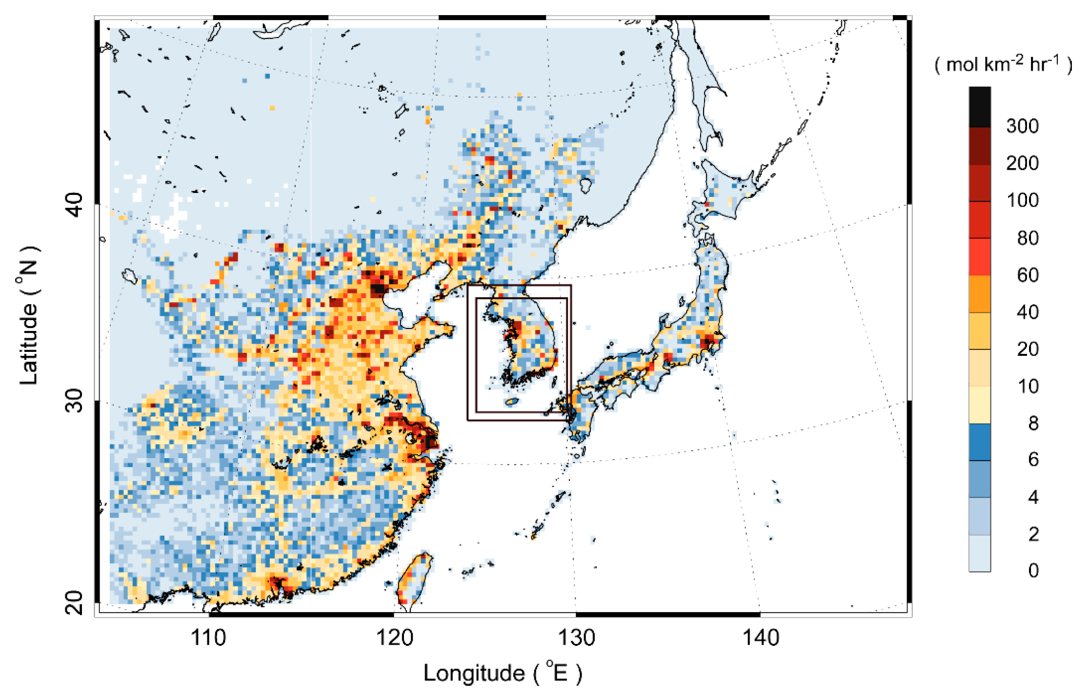
Figure 2.
The size distribution of the Aura/OMI pixels passed over the South Korean region (126°E–130°E, 34°N–38°N). The solid line denotes cumulative frequency in percentage. A median size of the overpassing pixels on a day was selected as a representative pixel size of the day. Total 33 days are analyzed. The shaded area indicates a range of the cities’ sizes in South Korea.

Figure 3.
(a) The spatial distribution of anthropogenic NOX emissions used for the simulations of the WRF-Chem and WRF/CMAQ models. A and P denote the highly urbanized area sources and the isolated point sources in South Korea, respectively. (b) A comparison of the annual NOX emissions of the selected area and point sources with their urbanized area. The source area of the point emissions is fixed by 3×3 km2 for clarity.
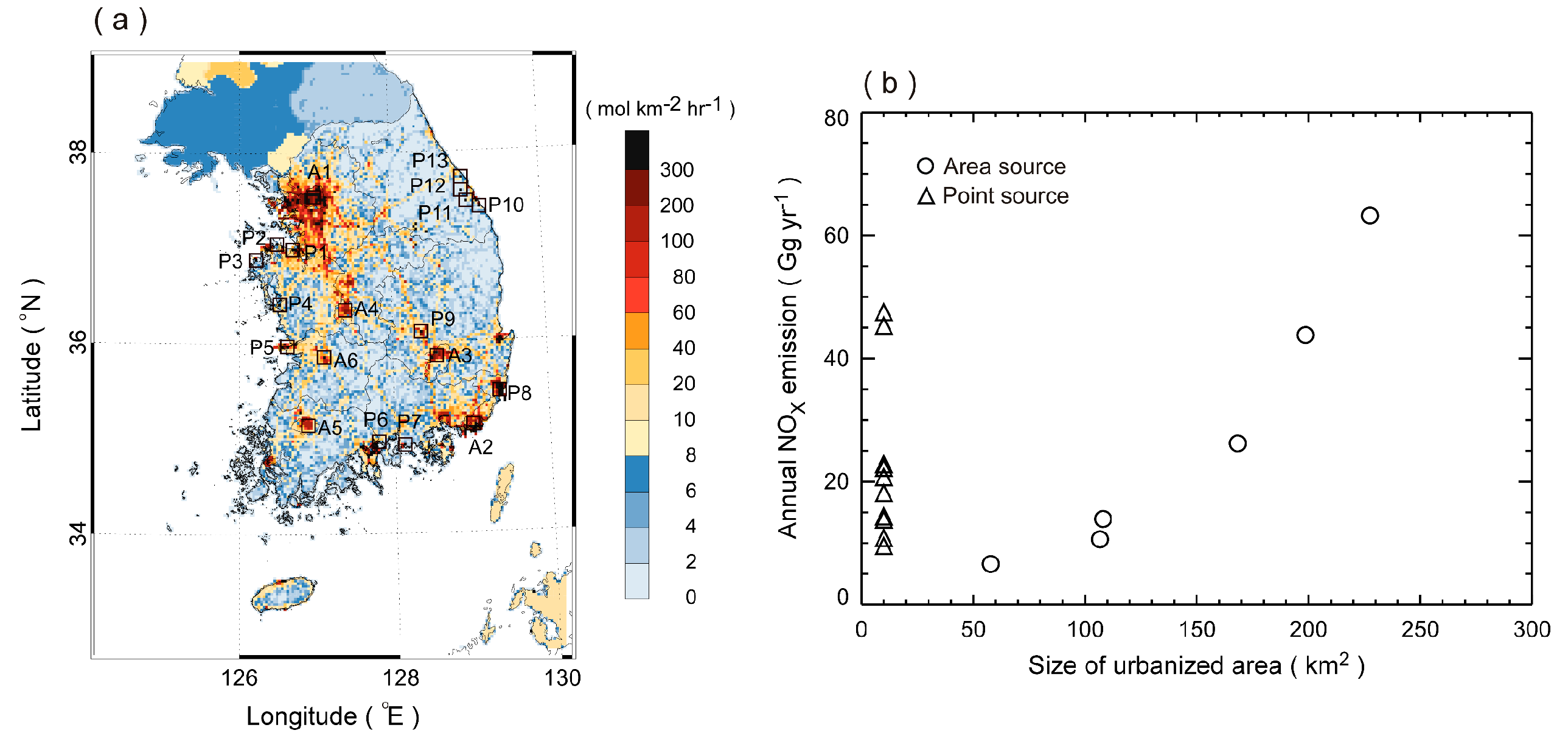
Figure 4.
The spatial distributions of tropospheric NO2 VCD over the South Korean region averaged for a period of January, April, July, and October 2015. (a) KNMI OMI NO2 VCD, (b) WRF-Chem modeled NO2 VCD, and (c) WRF/CMAQ modeled NO2 VCD.
Figure 4.
The spatial distributions of tropospheric NO2 VCD over the South Korean region averaged for a period of January, April, July, and October 2015. (a) KNMI OMI NO2 VCD, (b) WRF-Chem modeled NO2 VCD, and (c) WRF/CMAQ modeled NO2 VCD.
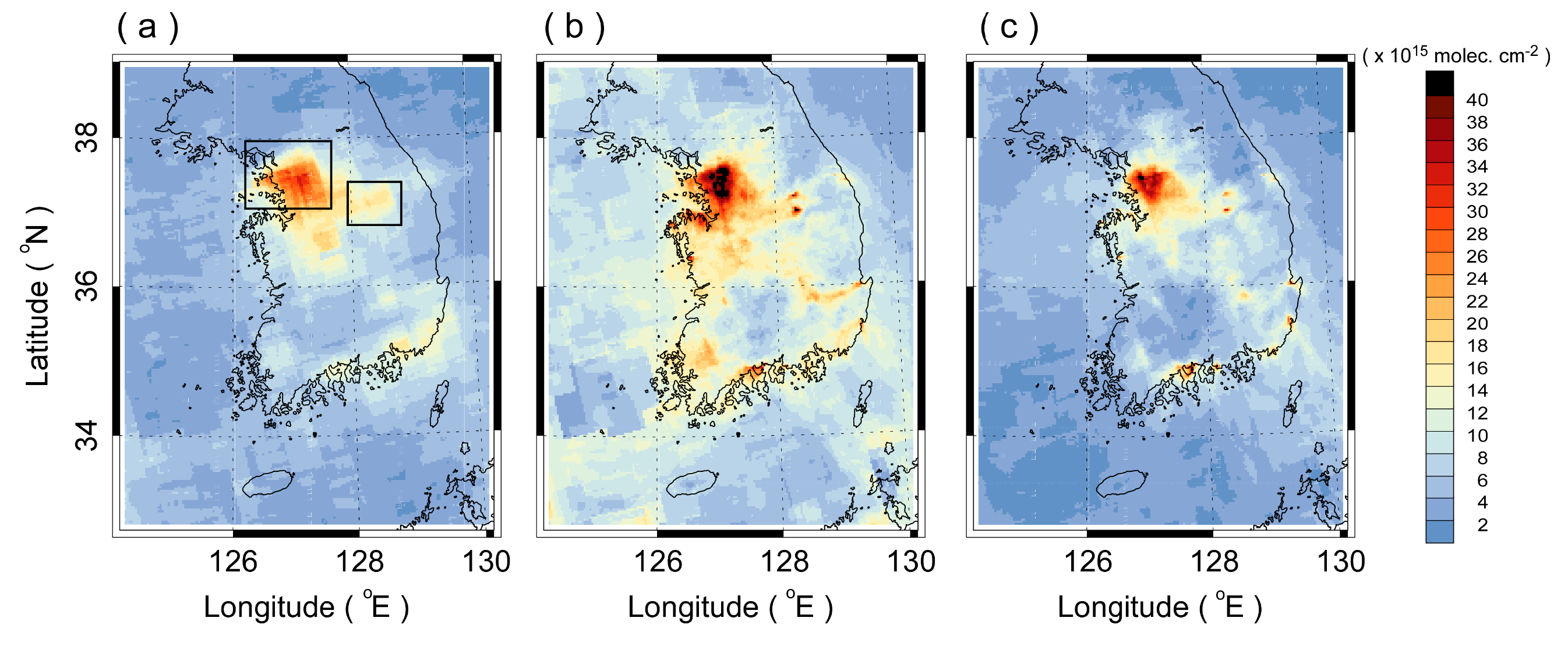
Figure 5.
A comparison of the monthly mean KNMI OMI-detected and modeled NO2 VCD over South Korea. The atmospheric NO2 VCD were averaged over the South Korean region (126°E–130°E; 34°N–38°N). The vertical bar in the KNMI OMI data denotes 1-sigma error.
Figure 5.
A comparison of the monthly mean KNMI OMI-detected and modeled NO2 VCD over South Korea. The atmospheric NO2 VCD were averaged over the South Korean region (126°E–130°E; 34°N–38°N). The vertical bar in the KNMI OMI data denotes 1-sigma error.

Figure 6.
The spatial distributions of the fine-scale reconstructed OMI NO2 VCD over the South Korean region obtained by applying the spatial-weight kernels from (a) WRF-Chem and (b) WRF/CMAQ.
Figure 6.
The spatial distributions of the fine-scale reconstructed OMI NO2 VCD over the South Korean region obtained by applying the spatial-weight kernels from (a) WRF-Chem and (b) WRF/CMAQ.

Figure 7.
The spatial distributions of the re-gridded and the reconstructed OMI NO2 VCD over (a–c) Seoul metropolitan area and (d–f) an area with industrial complexes. (a and d) re-gridded KNMI OMI NO2 VCD, (b and e) reconstructed OMI NO2 VCD using the WRF-Chem, (c and f) reconstructed OMI NO2 VCD using the WRF/CMAQ.

Figure 8.
A comparison of (a) the modeled NO2 VCD and (b) the reconstructed OMI NO2 VCD by the WRF-Chem and WRF/CMAQ models over the South Korean region. The modeled NO2 VCD in (a) were calculated by applying the KNMI OMI averaging kernels to the modeled vertical profiles of NO2 concentrations.
Figure 8.
A comparison of (a) the modeled NO2 VCD and (b) the reconstructed OMI NO2 VCD by the WRF-Chem and WRF/CMAQ models over the South Korean region. The modeled NO2 VCD in (a) were calculated by applying the KNMI OMI averaging kernels to the modeled vertical profiles of NO2 concentrations.
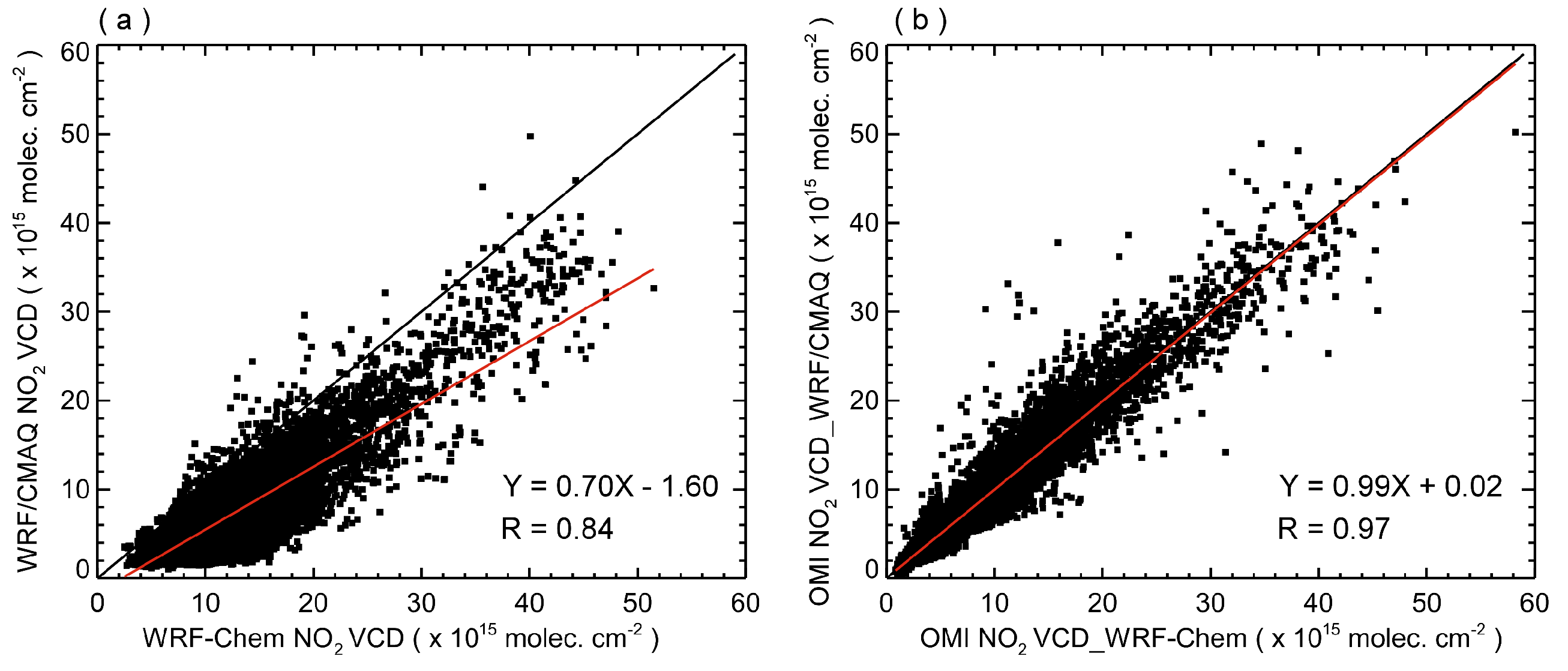
Figure 9.
(a) The spatial distribution of the reconstructed OMI NO2 VCD over the South Korean region and (b) the frequency distribution of the grid-scale normalized absolute difference defined as .
Figure 9.
(a) The spatial distribution of the reconstructed OMI NO2 VCD over the South Korean region and (b) the frequency distribution of the grid-scale normalized absolute difference defined as .
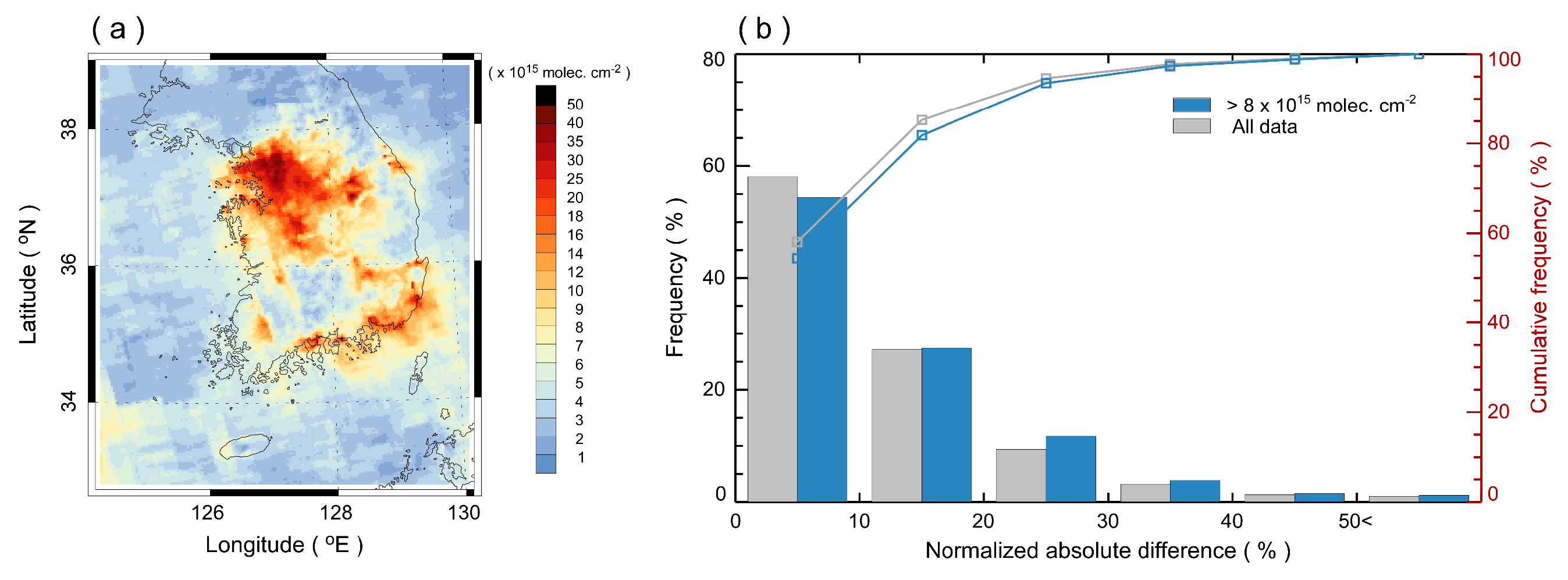
Figure 10.
A comparison of the re-gridded and reconstructed OMI NO2 VCD in terms of an averaging box size for (a) Seoul metropolitan area and (b) a site with cement industrial facilities in South Korea. The normalized absolute difference of the reconstructed OMI NO2 VCD is given for (c) 6 urbanized area sources and (d) 13 isolated point sources. Solid lines in (c) and (d) represent the mean normalized absolute difference for the urbanized area sources and the isolated point sources.

Figure 11.
A comparison of re-gridded and reconstructed OMI NO2 VCD on an effective spatial resolution for (a) 6 urbanized area sources and (b) 13 isolated point sources in South Korea.
Figure 11.
A comparison of re-gridded and reconstructed OMI NO2 VCD on an effective spatial resolution for (a) 6 urbanized area sources and (b) 13 isolated point sources in South Korea.

Figure 12.
A comparison of the re-gridded and reconstructed OMI NO2 VCD of the 13 major isolated point sources in South Korea against their annual NOX emissions. The vertical bar denotes the downscaling uncertainty estimated for the fine-scale reconstructed OMI NO2 product.
Figure 12.
A comparison of the re-gridded and reconstructed OMI NO2 VCD of the 13 major isolated point sources in South Korea against their annual NOX emissions. The vertical bar denotes the downscaling uncertainty estimated for the fine-scale reconstructed OMI NO2 product.


Table 1.
The configuration of the physical and chemical processes in the WRF-Chem and WRF/CMAQ models.
Table 1.
The configuration of the physical and chemical processes in the WRF-Chem and WRF/CMAQ models.
| Process | WRF-Chem (V3.9.1) | WRF/CMAQ (V3.6.1/V4.7.1) |
|---|---|---|
| Shortwave radiation | Goddard [58] | Dudhia [64] |
| Longwave radiation | RRTM [59] | |
| Turbulence | YSU [60] | |
| Land surface processes | Noah LSM [61] | |
| Microphysics | WSM3 [62] | |
| Cumulus parameterization | New Grell-3D | Kain-Fritsch [63] |
| Gas-phase chemistry | RACM [65] | SAPRC-99 [68] |
| Aerosol mechanism | MADE [66]/SORGAM [67] | AERO5 [69] |
| Anthropogenic emission | MICS-Asia 2010 [71] | |
| Biogenic emission | MEGAN-2 [73] |
© 2019 by the authors. Licensee MDPI, Basel, Switzerland. This article is an open access article distributed under the terms and conditions of the Creative Commons Attribution (CC BY) license (http://creativecommons.org/licenses/by/4.0/).
Share and Cite
MDPI and ACS Style
Lee, J.-H.; Lee, S.-H.; Kim, H.C. Detection of Strong NOX Emissions from Fine-scale Reconstruction of the OMI Tropospheric NO2 Product. Remote Sens. 2019, 11, 1861. https://doi.org/10.3390/rs11161861
AMA Style
Lee J-H, Lee S-H, Kim HC. Detection of Strong NOX Emissions from Fine-scale Reconstruction of the OMI Tropospheric NO2 Product. Remote Sensing. 2019; 11(16):1861. https://doi.org/10.3390/rs11161861
Chicago/Turabian StyleLee, Jae-Hyeong, Sang-Hyun Lee, and Hyun Cheol Kim. 2019. "Detection of Strong NOX Emissions from Fine-scale Reconstruction of the OMI Tropospheric NO2 Product" Remote Sensing 11, no. 16: 1861. https://doi.org/10.3390/rs11161861
Note that from the first issue of 2016, this journal uses article numbers instead of page numbers. See further details here.