An Analysis of Ground-Point Classifiers for Terrestrial LiDAR


Department of Geography, Environment & Geomatics, The University of Guelph, 50 Stone Rd. E, Guelph, ON N1G 2W1, Canada
*
Author to whom correspondence should be addressed.
Remote Sens. 2019, 11(16), 1915; https://doi.org/10.3390/rs11161915
Submission received: 16 July 2019
/
Revised: 2 August 2019
/
Accepted: 12 August 2019
/
Published: 16 August 2019
(This article belongs to the Special Issue Remote Sensing: 10th Anniversary)
Abstract
:Previous literature has compared the performance of existing ground point classification (GPC) techniques on airborne LiDAR (ALS) data (LiDAR—light detection and ranging); however, their performance when applied to terrestrial LiDAR (TLS) data has not yet been addressed. This research tested the classification accuracy of five openly-available GPC algorithms on seven TLS datasets: Zhang et al.’s inverted cloth simulation (CSF), Kraus and Pfeiffer’s hierarchical weighted robust interpolation classifier (HWRI), Axelsson’s progressive TIN densification filter (TIN), Evans and Hudak’s multiscale curvature classification (MCC), and Vosselman’s modified slope-based filter (MSBF). Classification performance was analyzed using the kappa index of agreement (KIA) and rasterized spatial distribution of classification accuracy datasets generated through comparisons with manually classified reference datasets. The results identified a decrease in classification accuracy for the CSF and HWRI classification of low vegetation, for the HWRI and MCC classifications of variably sloped terrain, for the HWRI and TIN classifications of low outlier points, and for the TIN and MSBF classifications of off-terrain (OT) points without any ground points beneath. Additionally, the results show that while no single algorithm was suitable for use on all datasets containing varying terrain characteristics and OT object types, in general, a mathematical-morphology/slope-based method outperformed other methods, reporting a kappa score of 0.902.
1. Introduction
Raw light detection and ranging (LiDAR) data is represented in a 3D point cloud where each point represents the return of a laser pulse from a reflected surface, be it the ground or any off-terrain (OT) objects situated between the sensor and the ground [1]. Common OT objects include trees, crops, utility infrastructures, and built objects like buildings. Importantly, airborne LiDAR systems provide comprehensive ground coverage, even under dense forest canopy [2]. Due to the high sampling rate and relatively small laser footprint size, beams can often penetrate through the canopy to reach the sub-canopy and ground surface beneath [3,4].
While initially developed for military applications in the 1960s, commercially available LiDAR sensors have been available since the 1990s. In recent years, reductions in both scanner cost and size has enabled many new applications [5]. In forestry science, LiDAR data has been used for tree and crown height measurements [6] and large-scale biomass estimates [7]. For archeological purposes, LiDAR can be used to characterize the ground surface with centimeter-level vertical accuracy [8,9]. For hazards mapping, LiDAR can be used to predict areas prone to landslide [10,11], which can be further utilized for safety assessments for proposed pipeline segments [12]. For route planning, LiDAR can also be used for pedestrian pathfinding to ensure route accessibility in urban environments [13]. Given this wide range of applications, different LiDAR data collection platforms are often required.
Platforms for LiDAR data collection include terrestrial laser scanners (TLS) (e.g., static LiDAR-mounted tripods), mobile laser scanners (MLS) (e.g., mobile mapping vehicles), and airborne laser scanners (ALS) (e.g., aircrafts and unpiloted aerial vehicles (UAV)), and to a lesser extent, orbital platforms [14,15,16]. Each collection platform has a unique associated scanner orientation, scan angle, point spacing, and laser footprint size, resulting in differences in their collected data [14,15,16,17,18,19,20]. ALS data typically exhibits an even point density distribution [19,21], a well-defined ground surface, a point spacing of roughly 0.5 m [22], and a laser footprint size of 10 cm–25 m [23]. Notably, a laser footprint size this large enables the collection of multiple returned points from a single laser pulse [24]. Comparatively, TLS data exhibits a variable point density distribution [19], a relatively large amount of ground surface noise [25,26], a minimum point spacing of <1 mm [27], and a laser footprint size of roughly 3.5–18 mm at the time of exit [27,28]. Although some long-range TLS can still collect multiple returned points from a single emitted pulse, they are typically only collected far away from the scanner once the beam has diverged to an extent that it is likely to intersect multiple surfaces.
Ground-point classification (GPC) is a process that automatically classifies each point as either a ground point or an OT point, and these differences in data collection methods create several unique challenges when performing the GPC of TLS data. In ALS data, it can be assumed that any first or intermediate point return will belong to an OT object [29], and many GPC algorithms take advantage of this assumption by implementing an initial first pass classification to classify all first and intermediate returns as OT objects [30]. This same assumption about return order and vertical position does not hold for long-range TLS scanners with multi-return capability. Given the ground-level orientation and increasingly oblique angle of the emitted laser pulse from TLS, first, intermediate, and last returns have the same likelihood of being surface or OT returns. Furthermore, the relatively higher resolution data provided by TLS creates a distinctly noisy ground surface caused by short ground vegetation like grass [25,26]. It is often the case that OT points in TLS datasets are captured without ground-points beneath, e.g., where the top of a distant OT object is visible above a nearer object or ridge that obscures the ground surface on which the distant object is situated. This is problematic for many GPC methods, particularly TIN and slope-based methods, that rely on selecting the lowest elevations in local neighborhoods as ground-points [31,32].
Inaccuracies in the GPC of a LiDAR point cloud can lead to further inaccuracies in the digital elevation models (DEM) interpolated from these data and to the propagation of errors during subsequent analyses [33,34]. Reviews of ALS GPC performed by Sithole and Vosselman [35] and Meng et al. [36] have concluded that in general, surface-based classifiers are the most accurate. However, no comparative review of GPC algorithms has been performed for TLS data specifically, as existing methods were developed for use on ALS datasets. Because of this, practitioners and researchers that utilize TLS data are relying on recommendations for GPC methods that have been derived from research focused on the point classification of ALS data. However, due to the uniqueness of each collection platform, recommendations based on the results from one collection platform may not necessarily translate to other LiDAR collection platforms.
The purpose of this study is to investigate the performance of ALS-designed GPC techniques on TLS data. This will be achieved by testing five openly-available, ALS-designed GPC algorithms on seven TLS datasets containing a range of topographic characteristics and OT objects. Classification accuracy will be assessed based on the results of statistical analysis comparing the agreement between the classification results of each algorithm and manually classified reference datasets, as well as by visual analysis of areas of disagreement between the two datasets to identify specific terrain and object characteristics where the classifiers are most likely to fail.
2. General Approaches to GPC
GPC creates two subsets of points from the initial point cloud, one containing the points belonging to the ground surface, and one containing the points belonging to objects on or above the ground surface. Subsequently, the classified ground points can be interpolated to create a bare-earth DEM. Bare-earth DEMs are often used for the characterization of the ground surface beneath dense forest cover for applications like headwater stream [37] and wetland [38] mapping, archeological mapping [9,39], and historical landslide mapping [11]. Alternatively, the remaining characterized OT objects can be used for forest inventorying [5], individual tree health assessments [40], solar energy potential estimates [41], and even remote powerline inspections [42].
Common GPC methods can be broadly categorized as slope-based, mathematical-morphology-based, surface-based, segmentation-based, and deep-learning-based [35,43]. Slope-based GPC methods [44,45,46] assume that within a local neighborhood, variations in terrain slope will be gradual, whereas the change in slope between the ground and an OT object will be comparably higher. Points are classified using inter-point slope and height values as the determining parameters; a minimum inter-point slope threshold is set, and when the slope connecting any two points exceeds this value, the higher elevation point is classified as an OT point.
Mathematical-morphology-based classifiers [47,48,49,50] classify points by performing a series of erosion and dilation operations, which adjust point elevations based on height differences with local minima or maxima [47]. The two basic mathematical morphology operations of erosion and dilation are commonly used in conjunction to perform opening (erosion followed by a dilation), closing (dilation followed by an erosion), or white top-hat (subtracting the opening surface from the DEM) operations [47]. These methods are sometimes combined with other approaches, most commonly slope-based GPC methods.
Surface-based classifiers iteratively approximate the ground surface by classifying ground points based on a modelled 3D buffer zone placed around local neighborhood minima points within the parametric surface [35]. Importantly, unlike slope- and mathematical-morphology-based classifiers, which aim to identify and remove OT points from the dataset, surface-based classifiers aim to iteratively approximate the ground surface by identify ground points within the dataset. There are three types of surface classifiers, including interpolation, triangulated irregular network (TIN), and active shape modelling [35,36]. Interpolation-based classifiers [51,52,53] iteratively densify initially selected ground points to gradually create a surface that represents the actual ground surface [43]. TIN-based classifiers, like that by Axelsson [54], begin by creating an initial sparse TIN using neighborhood minima points; points are then progressively added into the TIN if they meet user-defined slope and distance thresholds. Active shape models [55,56] float a membrane up toward the surface of a point cloud that clings to ground surface points; user-defined cloth rigidity and resolution parameters determine which points are clung to when creating the final surface.
Segmentation-based classifiers [57,58,59,60] typically cluster points together either by (1) clustering points that can be fit to the same modeled pane, or (2) using a region growing technique [21]. It is assumed that any points that cluster above the minimum elevation cluster within its neighborhood are OT points [35].
Deep-learning-based GPC approaches perform semantic segmentation using a neural network of classified point clouds [61]. Early approaches like that of Maturana and Scherer [62] first required that the point cloud data be transformed into regular 3D voxel grids. However, this was found to render the data into an unnecessarily large form, as well as introduce error into the datasets. Following this, Qi et al. [61] developed PointNet, an approach that directly uses the 3D point cloud format as its input and eliminates the need to voxelize the data. Further work by Qi et al. [63] saw the creation of the PointNet++ network, which utilizes a multiscale approach to classify the data. While initial applications of PointNet were largely indoor settings for object classification, more recent applications have seen this approach applied to large-extent ALS point clouds [64] and road scenes [65].
3. Materials and Methods
3.1. Data Collection
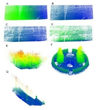
Following the guidelines for the testing of GPC algorithms suggested by Meng et al. [36], datasets exhibiting a range of topographic characteristics and OT objects were collected. Seven datasets with a range of slopes, elevations, object sizes, object densities, and surface coverings were collected around Guelph, Canada, and the surrounding area. These features were chosen because previous research has identified them as being inherently difficult to classify [35,36]. TLS data were collected using a multi-scan approach to reduce the effects of shadowing within the data and to provide a more complete coverage of the ground and OT objects. Scans were taken at different vantage points across each site and joined together using Leica’s Cyclone software (version 9.0, Leica, St. Gallen, Switzerland). Table 1 provides detailed descriptions of site characteristics. Figure 1 shows the seven datasets prior to GPC.
The very low corn (Figure 1A), low corn (Figure 1B), medium corn (Figure 1C), and high corn (Figure 1D) sites scans were taken progressively throughout the corn growing season at the same cornfield located in Guelph, Canada. Scans were taken from atop a raised embankment on the southern side of the front field margin scanning out toward the northern side. The site dimensions were roughly 93 m × 28 m, with point heights ranging from 0–0.20 m in the very low corn site, 0–0.60 m in the low corn site, 0–1.05 m in the medium corn site, and 0–1.95 m in the high corn site. The vegetated site (Figure 1E) scans were taken at a variably sloped forest outside of Guelph, Canada. The site dimensions were roughly 50 m × 172 m, with point heights ranging from 0–27 m. The garden site (Figure 1F) scans were taken at a circular garden at the University of Guelph, Canada. The site had a diameter of roughly 27 m and point heights ranging from 0–8 m. The road site (Figure 1G) scans were taken from the side of a road in Guelph, Canada. The site dimensions were roughly 14 m × 121 m, with point heights ranging from 0–14 m.
Data collection was completed using a Leica C10 ScanStation (Leica, Heerbrugg, Switzerland). This is a mid-range (300 m maximum) TLS with a scan rate capable of collecting up to 50,000 points per second with a 60 µrad × 60 µrad angular accuracy [27]. Scans were collected with a full 360° horizontal and 270° vertical field of view using a pulsed laser in the visible wavelength of 542 nm (green). At a range of 1–50 m, points are collected with a 6 mm positional accuracy and a 4 mm distance accuracy [27].
3.2. Data Reduction
TLS data frequently exhibit an extremely variable point density. Point density is generally low or moderate towards the outer portions of a scanned area but can be extremely high in the areas immediately adjacent to the scan stations [66]. Through careful planning of the number and placement of scan stations, it is possible to reduce the degree to which point density variability occurs. Multiple scans can then be joined together to decrease point density variability in the central area of the scans; however, point density will still be quite variable nearing and within the periphery of the datasets. Additionally, it is not unusual for a large proportion of the points in a TLS dataset to lie within this oversampled region a few meters distance surrounding each scan station. Therefore, prior to GPC, areas of extremely high point density were thinned from the sample datasets using a voxel-based data reduction method. This pre-processing step allowed for the GPC algorithms to be tested without the computational burden of having to process the oversampled ground surrounding each of the scan stations. The data reduction method worked by partitioning space into regular cube voxels (with 0.25 m sides), identifying voxels with point densities greater than an allowable maximum (10,000 points/m3), and then thinning the voxel points by removing every nth point, where n was calculated to yield the maximum allowable density. Notably, this voxel-based data reduction approach had the advantages of: (1) not affecting areas with data densities lower than the threshold, and (2) better preserving OT objects than alternative 2D gridding-based methods (note that 2D cells containing OT objects have high point densities and will therefore disproportionately thin OT points, which would be unsuitable for this study).
3.3. Evaluated GPC Algorithms
For this study five publicly available GPC algorithms were tested on collected TLS data. These algorithms were selected because of their open availability to researchers and practitioners alike. Table 2 outlines the broad methods used by each algorithm. A detailed description of each algorithm can be found below.
3.3.1. Zhang et al.’s Inverted Cloth Simulation (CSF)
The CSF classifier is a surface-based active shape model classifier that can be visualized as a cloth falling down onto an inverted point cloud and clinging to ground-points. The cloth resolution is first set to determine the distance between each cloth particle node. The shape of the cloth is then determined by a three-step process including both external (gravity) and internal (cloth rigidity) forces [56]. Throughout this process, cloth particles are set as either movable or immovable as their locations are finalized. The first step only considers the force of gravity as the cloth falls down onto the inverted surface. However, due to the displacement caused by gravity some cloth particles may end up below the ground surface. These particles are set as movable. The second step identifies these particles that have fallen below the ground surface and raises them up to the ground surface. These points are then set as immovable. The third step considers the internal forces of the cloth like rigidity and adjusts any remaining particles accordingly based on neighboring particle interactions. Points are then identified as ground if they fall within a set threshold distance from the calculated cloth surface. This process iterates until either the maximum set number of iterations is exceeded, or all points lie within the set ground threshold distance [56]. A more detailed description of this algorithm can be found in Zhang et al. [56]. This classifier was implemented in the CloudCompare software package (version 2.9.1, Télécom ParisTech, France).
3.3.2. Kraus and Pfeiffer’s Hierarchical-Weighted Robust Interpolation Classifier (HWRI)
This is a surface-based classifier that interpolates the ground surface using weighted linear prediction. The process is iterative and first calculates a rough ground surface approximation giving equal weights to all points. This initial approximation lies somewhere between the ground surface and OT objects. The residuals of each point in relation to the initial approximate ground surface are then calculated. It is assumed that ground points will be below the surface and will have negative residuals, and OT points will lie above the surface and will have positive residuals. These residuals are then used to compute weights for each point height measurement and are put into a weighted function that assigns larger weights to negative values (ground points), and smaller weights to positive values (OT points) [67]. This is an iterative process that updates the modelled ground surface after each iteration. The intermediate ground surface is completed once the user-defined number of iterations have completed. All points that then lie within the boundaries of the defined g (lower limit point boundary) and w (upper limit point boundary) parameter values are classified as ground points. A more detailed description of this algorithm can be found in Kraus and Pfeiffer [67]. This classifier was implemented in the FUSION/LDV LiDAR analysis software package (version 3.8, USDA Forest Service, Corvallis, United States).
3.3.3. Axelsson’s Progressive TIN Densification Filter (TIN)
The progressive TIN densification classifier is a surface-based classifier that begins by selecting neighborhood minima as seed points to create an initial sparse TIN [54]. Points are then added to the TIN through an iterative densification process that adds points if they fall below two defined thresholds: points must be below a determined distance range to the nearest triangle facet and below an angular threshold to the nearest triangle node [54]. Histograms are then derived from the distance and angular values of each point added to the TIN. The parameter threshold values for inclusion in the TIN are updated after each iteration using the median histogram values of the previously added points [54]. A more detailed description of this algorithm can be found in Axelsson [54]. This classifier was implemented in the LAStools software package (version 180731, rapidlasso GmbH, Gilching, Germany).
3.3.4. Evans and Hudak’s Multiscale Curvature Classification (MCC)
MCC is a surface-based classifier that gradually interpolates the ground surface by classifying points as OT objects if they surpass a user defined curvature threshold value calculated from an interpolated thin-plate spline surface. This is a multiscale approach that implements a user-defined scale parameter [52]. The curvature threshold for removal is also increased as it progresses to each new scale. Iterations continue for each scale until the remaining returns being classified as ground reach <1%, <0.1%, and <0.01% for each of the three scales, respectively [52]. A more detailed description of this algorithm can be found in Evans and Hudak [52]. This classifier was implemented in the MCC-LiDAR command line software application (version 2.1, U.S. Forest Service, Fort Collins, United States).
3.3.5. Vosselman’s Modified Slope-Based Filter (MSBF)
The MSBF is a mathematical-morphology-based/slope-based classifier that first implements a white top-hat transform to normalize initial differences in ground elevation. A minimum inter-point slope threshold is then set, and any point whose angle to the nearest point exceeds this value is excluded from the ground surface. While most slope-based classifiers now use a variable inter-point slope value for point classification, the initial ground surface normalization performed by the white top-hat transform allows for the use of a single constant inter-point slope value. An additional inter-point height threshold is set to exclude points greatly above others in its neighborhood. A more detailed description of this algorithm can be found in Vosselman [44]. This algorithm was implemented in the WhiteboxTools software package (version 0.15, University of Guelph, Canada).
3.3.6. Selection of Techniques to be Evaluated
Four surface-based methods were selected for testing and only one slope-based/mathematical-morphology based method. While no segmentation-based methods were included in this comparison, segmentation-based GPC techniques typically do not handle the classification of uneven point density well [68] and would likely not be well suited for the classification of areas of low point density inherent of the periphery of TLS datasets. Four surface-based methods were considered as the diversity between the way surface-based GPC methods operate is quite high. These four algorithms were chosen as they are representative of the three subcategories of surface-based classifiers (interpolation, TIN, and active shape model). Conversely, only one slope-based/mathematical morphology-based method was considered for testing as there is less variability in the way that slope-based methods operate. One of the only major variations between different slope-based methods is in the way that they determine their inter-point slope threshold. This is typically done either by using a constant inter-point slope threshold, or a variable inter-point slope threshold that increases as the distance to the point increases. The MSBF method implements a constant slope threshold but differentiates itself from other slope-based methods by implementing an initial white top-hat transform on the data that normalizes the elevation values of the underlying terrain. Rather than implementing a variable slope threshold and modifying the slope threshold between points, the MSBF method modifies the initial ground elevation to allow for a single slope threshold to be applied to the entire dataset.
3.4. Algorithm Optimization and Accuracy Assessment
There are four possible outcomes when performing GPC on LiDAR data. The first is to correctly classify an OT point (true positive, TP); the second is to correctly classify a ground point (true negative, TN); the third is to incorrectly classify a ground point as an OT point (false positive, FP); and the fourth is to incorrectly classify an OT point as a ground point (false negative, FN) [69]. To optimize the classification accuracy of each algorithm, comparisons were made between the automatically classified point clouds and manually classified reference datasets on a point-by-point basis. Reference datasets were created using the LAStools software package to visualize each dataset and manually classify each point as belonging to either the ground surface or an OT object. These reference datasets are available online at: https://sourceforge.net/projects/terrestrial-lidar-ref-datasets/files//?upload_just_completed =true.
The parameters of each GPC algorithm were adjusted to maximize their agreement with the reference data sets and then comparisons were made between the performances of these optimally classified datasets. Algorithm optimization was performed using the F1 statistic as a measure of algorithm performance. The F1 statistic calculates the harmonic mean of the precision and recall of the classification results. Precision is the ratio of correctly classified OT points to the total number of classified OT points; recall is the ratio of correctly classified OT points to the total number of actual OT points. In other words, these metrics measure the completeness (recall) and the correctness (precision) of the classification (e.g., a GPC algorithm that reported all points as OT points would have a recall of 1, but a low precision as all ground points would be misclassified). Mathematically the F1 statistic can be expressed as:
where precision is obtained using:
and recall is obtained using:
The F1 score ranges between 0 (poor classification performance) to 1 (perfect precision and recall). This metric places a higher level of importance on the correct classification of OT points (TP) and does not consider the correct classification of ground points (TN), except by extension (i.e., if the classification accuracy of OT points is low, ground points must also be poorly classified).
While the algorithm optimization was performed using the F1 score, the F1 score can be difficult to interpret across multiple datasets with differing numbers of ground points, OT points, and total points. As such, classification accuracy was assessed using the kappa index of agreement (KIA). The KIA is a measure of inter-rate agreement between qualitative items and is often considered a more robust measure of agreement than simple overall accuracy (i.e., percent correctly classified) as it considers the possibility of agreement occurring by chance [70]. Mathematically, the KIA can be expressed as:
where Po refers to the relative observed agreement among raters and Pe refers to the hypothetical possibility of agreement occurring by chance. A kappa score of 1.0 indicates a perfect classification and a kappa score of 0.0 indicates that the classification result is no better than what would be expected by chance. KIA can yield values less than 0.0 when the classifier performs poorer than random class assignment [71]. Additionally, the spatial distribution of classification accuracy was mapped to allow for visual inspection of the spatial context of algorithm performance, i.e., to identify specific areas within each site where classifiers performed well or poorly. For the very low corn, low corn, medium corn, and high corn datasets, the ground surface classified by each algorithm was subtracted from the reference dataset ground surface to observe height differences in their classified ground surfaces and the spatial distribution of these differences. For the vegetated, garden, and road datasets, the spatial accuracy was assessed using simple point classification agreement between each classified dataset and the references dataset.
4. Results
4.1. Overall Results
The overall accuracy (represented by the KIA) of the GPC algorithm performance provides useful information on the intra-site robustness of each algorithm regarding the range of features and topographic variations than can be handled within each site. The average and standard deviation of these values provides additional insight into the inter-site robustness of each algorithm regarding its performance across multiple sites with a range of topographic features and objects. Table 3 reports the kappa scores for each of the five tested GPC algorithms on each of the seven sites, and Table 4 reports the associated FP, FN, and total error (TE). TE refers to the combined number of FP and FN error points divided by the total number of points in the dataset.
The data in Table 3 and Table 4 were used to assess the overall GPC accuracy of the five tested algorithms on all seven datasets. The performance of the CSF classifier was relatively varied among the tested sites. Classification was performed poorly on the very low corn site, reporting a kappa score of 0.564. In particular, a large number of FN errors indicated an overrepresented ground surface (Table 4). Classification accuracy increased for the low, medium, and high corn sites; however, the CSF classifier still yielded the lowest kappa scores for the four corn sites. Conversely, the CSF classifier outperformed all other classifiers on the vegetated site, where both FP and FN errors remained low and a kappa score of 0.844 was achieved. The classification accuracy of the garden site was relatively low, reporting a kappa score of 0.812, the lowest overall for the site. The classification accuracy of the road site was relatively high, yielding a kappa score of 0.862, the second highest overall for the site. The CSF classifier reported the lowest overall average kappa score of 0.796.
The HWRI classifier performed poorly on the very low corn site, reporting a kappa score of 0.577. The FP error was relatively low for this site, indicating that nearly all the OT points were correctly classified. However, FN error was also high for this site, indicating that a large portion of ground points were also classified as OT points (Table 4). Classification accuracy increased for the low, medium, and high corn sites and the sites were classified well. Classification of the vegetated site demonstrated poor performance, with a kappa score of 0.662, which was the lowest for the site. The HWRI method yielded relatively accurate classifications of the garden and road sites, with the third highest kappa score among tested methods on the garden site, and the fourth highest kappa score among the tested methods on the road site. Overall, this classifier reported the second lowest average kappa score of 0.812 accompanied by a relatively high standard deviation of 0.127, indicating a highly variable classification performance with differing site characteristics.
The TIN classifier performed well on all four of the corn sites, reaching a peak classification accuracy at the low corn site with a kappa score of 0.958, the highest for the site. Classification accuracy was moderately high on the vegetated site, reporting a kappa score of 0.818, which was marginally lower than top-performing classification accuracy for the site of 0.844, reported by the CSF classifier. The TIN classifier also performed the best of all the tested methods on the garden site, reporting a kappa score of 0.934. However, the road site was classified relatively poorly by the TIN method, reporting a kappa score of 0.772, the lowest for the site. This resulted from an elevated occurrence of FP errors (Table 4), indicating a tendency to misclassify OT points as ground. On average, this classifier reported the second highest accuracy, with an average kappa score of 0.883.
The MCC classifier performed well on the low corn site, reporting a kappa score of 0.904, and performed moderately well on the very low, medium, and high corn sites. Classification accuracy was poor for the vegetated site, reporting a kappa score of 0.776, the second lowest for the site. This poor performance resulted from an abundance of FP errors at this site (Table 4). However, the MCC classifier performed relatively well on the road site, reporting a kappa score of 0.899, the highest for the site. On average, this classifier reported the third highest classification accuracy with an average kappa score of 0.864 and a low variability in performance among the test sites (Table 3).
The MSBF classifier performed well on all four of the corn sites, reporting kappa scores of 0.914, 0.953, 0.944, and 0.941 for the very low, low, medium, and high corn sites, respectively. Of all the tested algorithms, these were the highest kappa scores for the very low, medium, and high corn sites (Table 3). Classification accuracy was relatively high for the vegetated site with a kappa score of 0.842, just slightly lower than that of the CSF (Table 3). However, this classification performance resulted from a relatively high FP error of 16.5% and a low FN error of 2.07%, indicating an overly liberal classification of OT points. This classifier also performed moderately well on the garden and road sites, reporting kappa scores of 0.864 and 0.856, respectively. Overall, this classifier reported the highest average kappa score and relatively low inter-site variability in classification accuracy (Table 3).
4.2. Spatial Distribution of Algorithm Accuracy
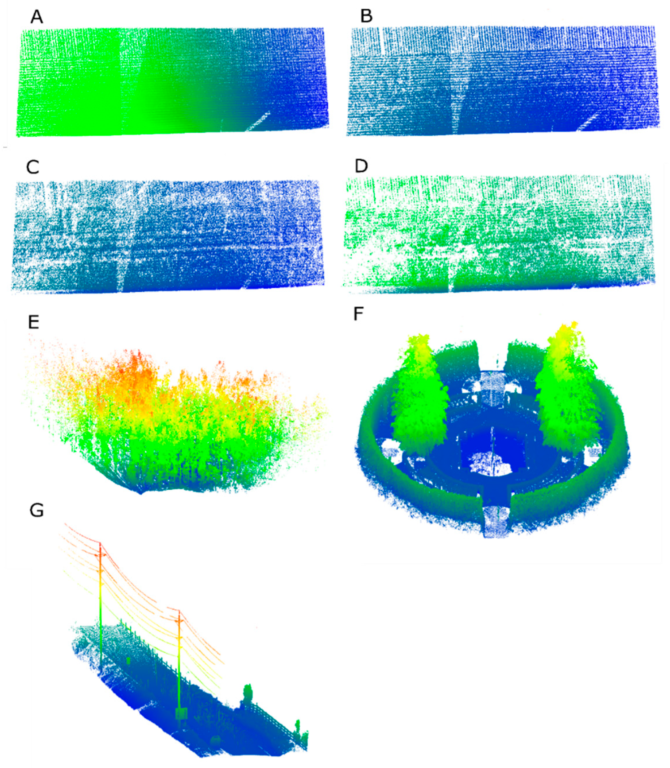
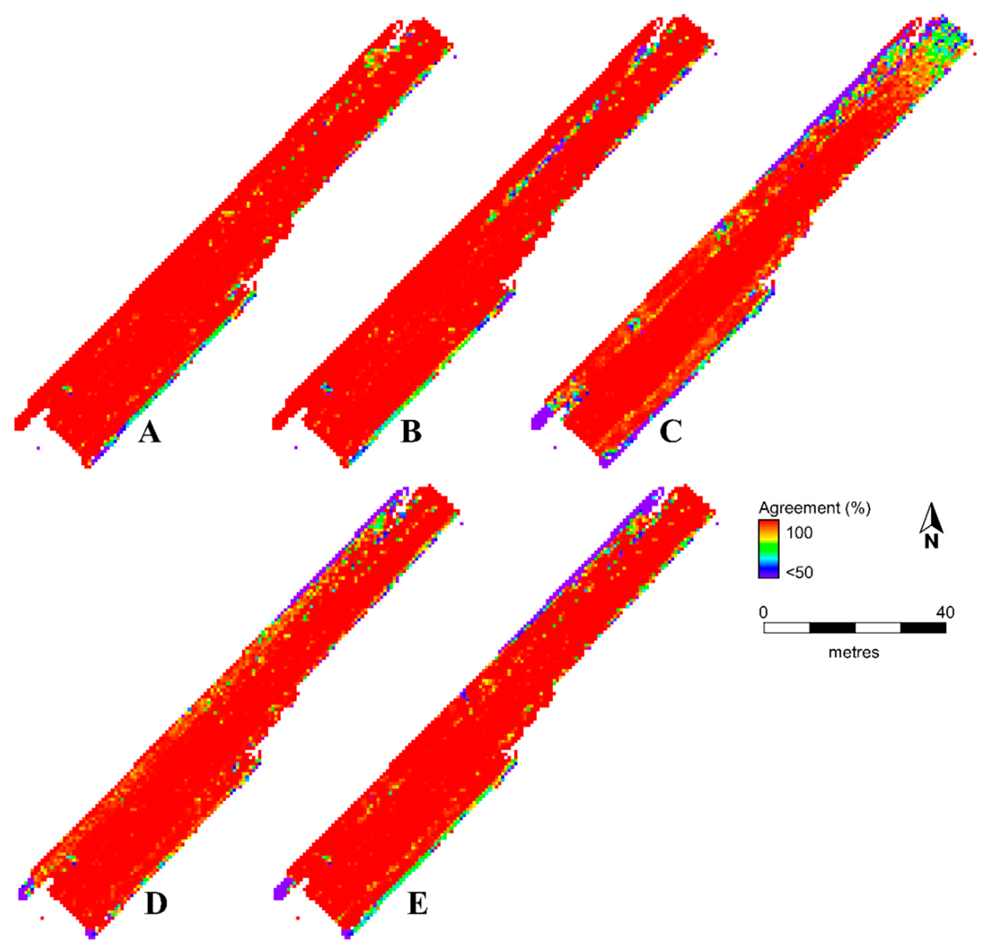
Figure 2, Figure 3, Figure 4 and Figure 5 show the spatial distribution of algorithm accuracy across each site. Whereas the overall classification accuracy results gave a sense of the robustness of each algorithm, the spatial distribution of accuracy throughout each site provided a better indication of the specific topographic characteristics and OT object types that each classifier was best suited to process. Figure 2 was created by subtracting the ground surface classified by each algorithm from the reference dataset ground surface. This shows the elevation differences between the algorithm classified ground surface and the actual ground surface. High residual values indicate an area of poor performance, and low residual values indicate an area of good performance. Figure 3, Figure 4 and Figure 5 were created via comparison, on a point-by-point basis, of the results of each algorithm classified dataset with the classified reference dataset. This shows specific areas within each site where the algorithms’ classification of the data differed from the reference dataset classification. For these figures, a high agreement with the reference dataset is favorable and indicates good performance by the classifier, and low agreement with the reference dataset indicates an area of poor performance by the classifier. It should be stressed that due to the inherent point density distribution variability of TLS data, total point values within each cell varied substantially throughout each raster. For the Vegetated site in particular, this tended to overrepresent the TE near the far edges of the dataset, where point density was low, and underrepresent the TE in the center of the dataset and in the area nearest the scanner, where point density was high.
Figure 2 provides examples of the spatial distribution of the GPC accuracy produced by the very low corn and high corn sites. The low corn site followed a similar pattern to the very low corn site, and the medium corn followed a similar pattern to the high corn site. For the very low corn and low corn sites, error for the CSF (Figure 2A) and HWRI classifications were distributed throughout the site following the rows of corn crops as the lowest portions of the crops were frequently misclassified as ground, resulting in many areas where the classified ground surface lay >0.05 m above the actual ground surface. Error was minimized for the MSBF (Figure 2B), TIN, and MCC classifications of these sites as these classifiers classified the low crops relatively well. As the number of ground points decreased in the medium and high corn sites, OT points were increasingly captured without ground points beneath them. The CSF (Figure 2C) and HWRI classifiers both handled the classification of these points relatively well, as the majority of the error was contained to the back of the data where ground and OT point density became sparse. Conversely, the MSBF (Figure 2D), TIN, and MCC classifiers frequently misclassified the base of these OT points, creating a false ground >2 m above the actual ground surface covering most of the site.
Figure 3 provides examples of the spatial distribution of accuracy for the Vegetated site. The TIN (Figure 3C), MCC (Figure 3D), and MSBF (Figure 3E) classifiers performed poorly near the edges of the site where OT points were captured without ground-points beneath. In contrast to this, the HWRI classifier performed well towards the edges of the site where this phenomenon occurred but performed poorly in the interior of the site (Figure 3B) where entire ravine ridges and hillsides were eroded away resulting in large holes in the classified ground data. Error within the CSF classification was relatively evenly dispersed, providing a good classification of both the edges and the interior of the site (Figure 3A).
Figure 4 shows examples of the spatial distribution of accuracy for the classification of the garden site. Error throughout this site was largely contained to three areas: the hedges encircling the entire site, raised flower beds throughout the site, and the pit (drained fountain) in the center of the site. The flat pathway between the hedges and flower beds was consistently classified well by all classifiers (Figure 4A–E). All classifiers except for TIN (Figure 4C) showed a significant amount of error when classifying the hedges and raised flower beds. The pit was characterized by flat vertical walls along the sides topped with curved ridges connecting them to the ground surface. The vertical walls were correctly classified by the MCC and MSBF classifiers and were classified moderately well by the TIN classifier. However, all classifiers misclassified the curved ridge on top (Figure 4A–E). Beneath the vertical walls were low outlier points created by double bounces within the fountain. These points were classified relatively well by the MCC and MSBF classifiers, moderately well by the CSF classifier, and were largely misclassified by the HWRI and TIN classifiers.
Figure 5 provides examples of the outputs of the spatial distribution of error for the road site. The grass-covered embankment on the upper left section of the site was classified relatively poorly by the TIN (Figure 5C) and MCC (Figure 5D) classifiers. While the HWRI classifier also produced a moderate amount of error in this area, it was contained along the upper ridge of the embankment (Figure 5B). Apart from the embankment, error within this site largely occurred along the edges of the site with the classification of the fences, roadside cable barriers, and utility poles. Classification of the utility poles and powerlines was performed poorly by the TIN classifier, whereas the MCC and MSBF classifiers classified the poles correctly, but misclassified sections of the powerlines. The bases of the utility poles were misclassified by the CSF and HWRI classifiers. Fences and roadside cable barriers were largely correctly identified as OT points by the CSF, HWRI, and MSBF classifiers; however, the bases of the structures were frequently misclassified as ground (Figure 5B). Additionally, outlier points created by cars driving along the road during the scan were correctly classified by all algorithms.
5. Discussion
5.1. Parameter Sensitivity Analysis
In general, the two parameters that had the largest impact on classification performance were the slope and height thresholds. Classifiers that utilize a height threshold parameter use variations in point height to approximate a ground surface, from which it is then assumed that any points lying above it are OT points. Conversely, an inter-point slope threshold classifies points as OT if the slope between neighboring points exceeds a set threshold. In ALS data, where it can be assumed that OT points will lie at least 0.5 m off the ground [56], a height threshold parameter may indeed be an appropriate method for GPC. However, in TLS data where OT points can lie mm above the ground, selecting an appropriate threshold is challenging and often results in the misclassification of low OT points, such as those in the CSF classification of the four corn sites.
5.2. Ground-Point Classifier Selection
Previous research on the classification of ALS data suggests that while the most appropriate GPC algorithm will vary depending on the terrain characteristics and OT objects in the site, in general, surface-based classifiers tend to outperform other methods [35,36]. However, results from this study have shown that overall, the MSBF classifier (a mathematical morphology and slope-based classifier) reported the highest classification accuracy (Table 3). A possible explanation for the increased accuracy of this type of classifier over surface-based classifiers was the increased detail of the ground surfaces captured by TLS. While ALS data can provide a more consistent coverage of the ground surface throughout the entire scanned scene, TLS provides a far more detailed characterization of the surface and the surrounding area [72]. This can be problematic when scanning grassed landscapes as it can add an unnecessary amount of complexity to the ground surface. Furthermore, Fan et al. [25] noted that when scanning grass-covered landscapes, the average penetration depth into the grass was only 35–40%. This indicates that the ground captured in TLS scans of grassed landscapes was often actually a highly complex surface created at somewhat of a midway point between the actual ground surface and the top of the grass.
Given that surface-based classifiers work by approximating the ground surface by identifying possible ground points, the increased complexity of the ground surface would make this process more challenging. Meanwhile, mathematical-morphological/slope-based classifiers, which aim to iteratively identify and remove OT objects until all that remains is the ground surface, would be relatively unaffected by this. This could also explain why in the garden site, surface-based classifiers like HWRI, TIN, and MCC outperformed the MSBF classifier, as this was the only site where the majority of the ground surface was not covered by grass or short vegetation.
While the MSBF classifier reported the highest overall classification accuracy, a large FP or FN error reported by other classifiers does not necessarily mean that the resulting DEM will be poor. Rather, this is determined by the distribution of the error throughout the landscape [33]. For example, the creation of FP errors where ground point density is high will have a relatively small effect on the resulting DEM as interpolation will fill in any gaps in the data. However, the creation of FN errors near the edge of the dataset where point density is low will add a degree of error into the created DEM.
5.3. Analysis of Difficult-to-Classify Terrain and Object Characteristics
The overall classification accuracy combined with the spatial distribution of classification error has allowed for the identification of several instances where certain types of classifiers tend to perform poorly. These include the classification of low vegetation, variably sloped terrain, outlier points, and areas where OT points are captured without ground points beneath.
Low vegetation and low objects have been previously identified as an inherently difficult feature to classify [35]. Due to their proximity to the ground it can be difficult to distinguish between the end of the ground surface and the beginning of an OT object. The CSF classifier consistently misclassified low vegetation and the base of OT objects. This can largely be attributed to the minimum threshold for OT point classification being 0.1 m. While this may be an appropriate minimum value for ALS data where OT points are typically at least 0.5 m from the ground [56], TLS collects data with a much smaller point spacing (<1 mm compared to 0.2–1 m for airborne systems [22,27]), meaning that OT points could be collected starting at just mm above the ground. The HWRI similarly misclassified low vegetation points in the very low corn site and reported an FP error of 0.03% and an FN error of 53.49%. This was likely the result of microtopographical ridges and burrows created in between the tillage mounds of the field occurring at the same scale as the misclassified vegetation. Pfeifer et al. [73] noted a similar phenomenon, albeit on a larger scale, when attempting to remove a low-lying building on the ridge of an embankment. There is typically a trade-off between the production of FP and FN errors. By parameterizing the classifier to conserve as much ground as possible (as is the case with the high amount of ground points in the very low corn site), OT points were erroneously included in the ground classification.
In addition to the difficulty provided by the classification of low vegetation points, the classification of points on variably sloped terrain poses a similarly large challenge to the GPC process. Interpolation-based classifiers like HWRI and MCC in particular struggled with the classification of terrain with variable slopes in the vegetated site, reporting FP errors of 24.09% and 21.15%, respectively (Table 4). Specifically, the HWRI classifier misclassified an entire section of ground along the steep slopes and ridges of the vegetated site (Figure 6A), confirming the findings of Lee and Younan [74] that linear prediction-based classifiers like HWRI frequently fail to classify terrain with steep or variable slopes. In contrast, the variable terrain of the vegetated site was handled well by the CSF classifier (Figure 6B). This classifier utilizes an additional post-processing step to identify areas of steep slope where cloth rigidity alone is not enough to accurately classify a point along the sloped surface [56]. The MSBF classifier also handled the classification of variably sloped terrain well. Typically, classifiers that implement a static slope threshold like that used by MSBF do not perform well on terrains with variable slopes as it is difficult to select a single appropriate slope value for an entire dataset [3]. However, the addition of the initial white-top hat transform normalizes any variability in terrain elevations before the classification begins, allowing for a single-slope threshold to be better applied to the entire dataset (Figure 6C).
In TLS data, variable sloped terrain can also result in the collection of OT points without any ground points collected beneath them. While in ALS data, it is often the case that as OT object density increases, ground point coverage decreases, this scenario is typically handled well as most classifiers assume that the lowest point in a neighborhood is the ground, regardless of how many points are collected [35]. However, in TLS, an increasingly oblique scanning angle coupled with variable terrain and increasing OT object density often captures OT points without any ground points beneath (e.g., where the top of a distant OT object is visible above a nearer object or ridge that obscures the ground surface on which the distant object is situated). The CSF and HWRI (Figure 7A) classifiers both minimized error when classifying OT points of this type in the high corn site.
The HWRI classifier utilizes an above/below surface offset parameter that determines the weights given to points a certain elevation above or below the approximated surface. Setting a larger below-surface offset parameter can give these points a smaller weight in the final ground surface calculation and have them correctly classified as OT. The CSF classifier uses a cloth rigidity function to better handle steep/variably sloped terrains. Given that this site has a relatively flat ground surface, by setting the rigidity parameter to high, these points can be easily identified as OT by their sharp increase in elevation. Conversely, classifiers like the TIN and MSBF (Figure 7B) classified these points relatively poorly, as both classifiers initialize their classification using the lowest neighborhood minima points as assumed ground points. The result is that the bottom of the scanned portion of OT objects, which often lie significantly above the ground, are classified as ground points.
While the collection of OT points without any ground points beneath them poses a challenge for the GPC process, low outlier points collected beneath the actual ground surface can similarly be problematic. High outliers are points that are captured unnaturally high in the scanned scene. As expected, high outliers were handled well by all classifiers. Conversely, low outliers are erroneous points that lie below the surface of the scanned scene and are caused by things like double bounce returns. Figure 8 shows an example of this where double bounces reflecting off the walls of the drained fountain in the center of the garden site have created low outlier points mimicking the vertical walls of the fountain. These points were handled well by the MSBF classifier (Figure 8B), whereas iterative classifiers, like HWRI and TIN, were particularly susceptible to FN errors in this area. The poor performance of the HWRI classifier can be explained by the initial roughly approximated ground surface that is created by averaging the elevations of points in the same z-plane. Points that lie below this surface are then considered to be ground points and are given a larger weight in the proceeding function, and points that lie above this surface are assumed to be OT points and are given a smaller weight. Given the high density of outlier points below the actual ground surface in this area and the large weights that they were assigned, these points skewed the calculation of the final ground surface to be well below the actual surface, causing the outlier points to be misclassified as ground. Similarly, the poor performance of the TIN classifier in this area can be attributed to the way it initialized the iterative interpolation process by creating an initial sparse TIN from the neighborhood minima. In a site containing low outlier points, these points become the seed points for the initialization of the TIN, which results in their misclassification as ground points.
5.4. Point Density Variability
Data thinning was performed to reduce the total amount of points requiring classification. This was done by restricting the maximum number of points per voxel to 10,000. Although this resulted in a significant reduction of data points in the highly dense areas nearby the scanner, it did not address the issue of variable point densities throughout the dataset. Given that point densities were still highly variable throughout the sites (a 1 m cell could contain anywhere from 30–30,000 points), the results of the spatial distribution of error were somewhat distorted as total error was overrepresented in cells near the edges of the site that contain a smaller number of total points.
This can prove problematic for the interpretation of some of the results presented by this research. For example, while the kappa score for the HWRI classification of the vegetated site indicates a poorly performed classification, Figure 3B appears to show a well classified site. Similarly, while the kappa score for the MSBF classification of the vegetated site was only marginally lower than the top classification, Figure 3E appears to show a poorly performed classification of the site. This was because for the HWRI classification, error was largely contained to a few relatively small areas in the center of the site where the point density was high (Figure 3B), whereas for the MSBF classification, error was largely contained to the edges of the dataset where point density was low (Figure 3E). Additionally, because point density is directly affected by the distance from the scanner, the point collection distance from scanner can also be considered a factor directly affecting terrestrial LiDAR GPC accuracy.
6. Conclusions
Current algorithms developed for ALS GPC were tested on TLS data. Existing comparisons performed on ALS data by Sithole and Vosselman [35] and Meng et al. [36] have shown that while choosing an appropriate algorithm for GPC will vary by site, in general, surface-based methods performed the best. Results from our study have shown that while choosing an appropriate algorithm for performing GPC is still site-specific, in general, mathematical-morphological-based/slope-based methods, like the MSBF, outperformed surface-based methods. The MSBF classifier reported an overall average kappa score of 0.902, whereas the CSF, HWRI, TIN, and MCC methods reported as overall average kappa scores of 0.796, 0.812, 0.883, and 0.864, respectively. The overall greater classification accuracy of MSBF was likely owed to the increased complexity of vegetated ground surfaces captured by TLS. While the MSBF classifier reported the highest overall accuracy, it is important to note that there were several terrain characteristics and OT object types where other classifiers outperformed the MSBF. While the CSF classifier performed poorly for the classification of low vegetation, it performed well in areas where OT points were collected without ground points beneath and areas of steep/variably sloped terrain. While the HWRI classifier misclassified low outlier points and tended to underrepresent the ground surface in areas of steep/variably sloped terrain, it also showed promise for the classification of OT points without ground points beneath. The TIN classifier performed well in the classification of less complex and flat surfaces while still performing moderately well in the classification of steep/variably sloped terrain. While the MCC classifier performed poorly for the classification of steep/variably sloped terrain, the classification of the road site containing both a simple flat ground surface and a complex vegetated ground surface was performed well.
Author Contributions
Conceptualization, K.C.R. and J.B.L.; Data curation, K.C.R.; Formal analysis, K.C.R.; Funding acquisition, J.B.L. and A.A.B.; Investigation, K.C.R.; Methodology, K.C.R. and J.B.L.; Project administration, J.B.L.; Resources, K.C.R., J.B.L., and A.A.B.; Software, J.B.L.; Supervision, J.B.L.; Validation, K.C.R.; Visualization, K.C.R.; Writing—original draft, K.C.R.; Writing—review and editing, K.C.R., J.B.L., and A.A.B.
Funding
This research was funded by grants provided by The Natural Sciences and Engineering Research Council of Canada (NSERC; grant number 400,317) and The Canada Foundation for Innovation (CFI; grant number 46,477).
Acknowledgments
The authors would like to thank the anonymous reviewers. Their useful comments and suggestions led to an improved final draft of the paper. The authors would also like to thank Anthony Francioni for his help with the collection of the TLS datasets.
Conflicts of Interest
The authors declare no conflict of interest. The funders had no role in the design of the study; in the collection, analyses, or interpretation of data; in the writing of the manuscript, or in the decision to publish the results.
References
- Chang, Y.; Habiba, A.F.; Leeb, D.C.; Yomb, J.; Scanning, L.; Cloud, P. Automatic classification of lidar data into ground and non-ground points. Int. Arch. Photogramm. WG IV3 2000, 37, 457–462. [Google Scholar]
- Reutebuch, S.E.; Mcgaughey, R.J.; Andersen, H.; Carson, W.W. Accuracy of a high-resolution lidar terrain model under a conifer forest canopy. Can. J. Remote Sens. 2003, 29, 527–535. [Google Scholar] [CrossRef]
- Liu, H.; Wang, L. Mapping detention basins and deriving their spatial attributes from airborne LiDAR data for hydrological applications. Hydrological 2008, 45, 559–567. [Google Scholar] [CrossRef]
- Tompalski, P.; Coops, N.C.; White, J.C.; Wulder, M.A.; Yuill, A. Characterizing streams and riparian areas with airborne laser scanning data. Remote Sens. Environ. 2017, 192, 73–86. [Google Scholar] [CrossRef]
- Wallace, L.; Lucieer, A.; Watson, C.; Turner, D. Development of a UAV-LiDAR system with application to forest inventory. Remote Sens. 2012, 4, 1519–1543. [Google Scholar] [CrossRef]
- Coops, N.C.; Hilker, T.; Wulder, M.A.; St-Onge, B.; Newnham, G.; Siggins, A.; Trofymow, J.A. Estimating canopy structure of Douglas-fir forest stands from discrete-return LiDAR. Trees 2007, 21, 295–310. [Google Scholar] [CrossRef]
- Hese, S.; Lucht, W.; Schmullius, C.; Barnsley, M.; Dubayah, R.; Knorr, D.; Neumann, K.; Riedel, T.; Schröter, K. Global biomass mapping for an improved understanding of the CO2 balance—The Earth observation mission Carbon-3D. Remote Sens. Environ. 2005, 94, 94–104. [Google Scholar] [CrossRef]
- Bewley, R.H.; Crutchley, S.P.; Shell, C.A. New Light on an Ancient Landscape: LiDAR Survey in the Stonehenge World Heritage Site. Antiquity 2005, 79, 636–647. [Google Scholar] [CrossRef]
- Evans, D.H.; Fletcher, R.J.; Pottier, C.; Chevance, J.-B.; Soutif, D.; Tan, B.S.; Im, S.; Ea, D.; Tin, T.; Kim, S.; et al. Uncovering archaeological landscapes at Angkor using lidar. Proc. Natl. Acad. Sci. USA 2013, 110, 12595–12600. [Google Scholar] [CrossRef] [Green Version]
- Dlugosz, M. Digital Terrain Model ( Dtm ) As a Tool for Landslide Investigation in the Polish Carpathians. Versita 2012, 46, 5–23. [Google Scholar]
- Van Deen Eeckhaut, M.; Poesen, J.; Verstraten, G.; Vanacker, V.; Nyssen, J.; Moeyersons, J.; Van Beek, L.P.H.; Vandekerckhove, L. Use of LIDAR-derived images for mapping old landslides under forest. Earth Surf. Process. Landf. 2007, 32, 754–769. [Google Scholar] [CrossRef]
- Tao, C.V.; Hu, Y. Assessment of airborne Lidar and imaging technology for pipeline mapping and safety applications. In Proceedings of the Pecora 15/Land Satellite Information IV/ISPRS Commission I/FIEOS, Denver, CO, USA, 10–15 November 2002. [Google Scholar]
- Balado, J.; Díaz-Vilariño, L.; Arias, P.; Lorenzo, H. Point clouds for direct pedestrian pathfinding in urban environments. ISPRS J. Photogramm. Remote Sens. 2019, 148, 184–196. [Google Scholar] [CrossRef]
- Petrie, G.; Toth, C.K. Airborne and Spaceborne Laser Profilers and Scanner. In Topographic Laser Ranging and Scanning: Principles and Processing; Shan, J., Toth, C.K., Eds.; CRC Press: Boca Raton, FL, USA, 2008. [Google Scholar]
- Petrie, G.; Toth, C.K. Terrestrial Laser Scanners. In Topographic Laser Ranging and Scanning: Principles and Processing; Shan, J., Toth, C.K., Eds.; CRC Press: Boca Raton, FL, USA, 2008. [Google Scholar]
- Charlton, M.; Coveney, S.; McCarthy, T. Issues in Laser Scanning. In Laser Scanning for the Environmental Sciences; Heritage, G., Large, A., Eds.; John Wiley & Sons: Hoboken, NJ, USA, 2009. [Google Scholar]
- Abshire, J.B.; Sun, X.; Riris, H.; Sirota, J.M.; McGarry, J.F.; Palm, S.; Yi, D.; Liiva, P. Geoscience Laser Altimeter System (GLAS) on the ICESat mission: On-orbit measurement performance. Geophys. Res. Lett. 2005, 32, 1–4. [Google Scholar] [CrossRef]
- Schutz, B.E.; Zwally, H.J.; Shuman, C.A.; Hancock, D.; DiMarzio, J.P. Overview of the ICESat mission. Geophys. Res. Lett. 2005, 32, 1–4. [Google Scholar] [CrossRef]
- Perroy, R.L.; Bookhagen, B.; Asner, G.P.; Chadwick, O.A. Comparison of gully erosion estimates using airborne and ground-based LiDAR on Santa Cruz Island, California. Geomorphology 2010, 118, 288–300. [Google Scholar] [CrossRef]
- Young, A.P.; Olsen, M.J.; Driscoll, N.; Flick, R.E.; Gutierrez, R.; Guza, R.T.; Johnstone, E.; Kuester, F. Comparison of Airborne and Terrestrial Lidar Estimates of Seacliff Erosion in Southern California. Photogramm. Eng. Rem. Sens. 2010, 76, 421–427. [Google Scholar] [CrossRef] [Green Version]
- Vosselman, G.; Klein, R. Visualisation and structuring of point clouds. In Airborne and Terrestrial Laser Scanning; Vosselman, M.G., Mass, H.G., Eds.; CRC Press: Boca Raton, FL, USA, 2010; pp. 45–81. [Google Scholar]
- Rupnik, B.; Mongus, D.; Žalik, B. Point density evaluation of airborne LiDAR datasets. J. Univers. Comput. Sci. 2015, 21, 587–603. [Google Scholar]
- Silva, C.A.; Saatchi, S.; Garcia, M.; Labri, N.; Klauberg, C.; Meyer, V.; Jeffery, K.J.; Abernethy, K.; White, L.; Zhao, K.; et al. Comparison of Small- and Large-Footprint Lidar Characterization of Tropical Forest Aboveground Structure and Biomass: A Case Study From Central Gabon. IEEE J. Sel. Top. Appl. Earth Obs. Remote Sens. 2018, 11, 3512–3526. [Google Scholar] [CrossRef] [Green Version]
- Dassot, M.; Constant, T.; Fournier, M. The use of terrestrial LiDAR technology in forest science: Application fields, benefits and challenges. Ann. For. Sci. 2011, 68, 959–974. [Google Scholar] [CrossRef]
- Fan, L.; Powrie, W.; Smethurst, J.; Atkinson, P.M.; Einstein, H. ISPRS Journal of Photogrammetry and Remote Sensing The effect of short ground vegetation on terrestrial laser scans at a local scale. ISPRS J. Photogramm. Remote Sens. 2014, 95, 42–52. [Google Scholar] [CrossRef]
- Che, E.; Olsen, M.J. ISPRS Journal of Photogrammetry and Remote Sensing Fast ground filtering for TLS data via Scanline Density Analysis. ISPRS J. Photogramm. Remote Sens. 2017, 129, 226–240. [Google Scholar] [CrossRef]
- Leica Geosystems, A.G. Leica Leica ScanStation C10 The All-in-One Laser Scanner for Any Application; Leica Geosystems: Heerbrugg, Switzerland, 2011. [Google Scholar]
- Riegl Terrestrial Laser Scanning Products. 2018. Available online: http://www.riegl.com/products/terrestrial-scanning/ (accessed on 15 August 2019).
- James, L.A.; Watson, D.G.; Hansen, W.F. Using LiDAR data to map gullies and headwater streams under forest canopy: South Carolina, USA. Catena 2007, 71, 132–144. [Google Scholar] [CrossRef]
- Sharma, M.; Paige, G.B.; Miller, S.N. DEM Development from Ground-Based LiDAR Data: A Method to Remove Non-Surface Objects. Remote Sens. 2010, 2, 2629–2642. [Google Scholar] [CrossRef] [Green Version]
- Zhang, K.; Whitman, D. Comparison of Three Algorithms for Filtering Airborne Lidar Data Comparison of Three Algorithms for Filtering Airborne Lidar Data. Photogramm. Eng. Remote Sens 2005, 71, 313–324. [Google Scholar] [CrossRef]
- Meng, X.; Wang, L.; Silván-Cárdenas, J.L.; Currit, N. A multi-directional ground filtering algorithm for airborne LIDAR. ISPRS J. Photogramm. Remote Sens. 2009, 64, 117–124. [Google Scholar] [CrossRef] [Green Version]
- Fisher, P.E.F.; Tate, N.J.J. Causes and consequences of error in digital elevation models. Prog. Phys. Geogr. 2006, 30, 467–489. [Google Scholar] [CrossRef]
- Hutton, C.; Brazier, R. Quantifying riparian zone structure from airborne LiDAR: Vegetation filtering, anisotropic interpolation, and uncertainty propagation. J. Hydrol. 2012, 442–443, 36–45. [Google Scholar] [CrossRef]
- Sithole, G.; Vosselman, G. Experimental comparison of filter algorithms for bare-Earth extraction from airborne laser scanning point clouds. ISPRS J. Photogramm. Remote Sens. 2004, 59, 85–101. [Google Scholar] [CrossRef]
- Meng, X.; Currit, N.; Zhao, K. Ground Filtering Algorithms for Airborne LiDAR Data: A Review of Critical Issues. Remote Sens. 2010, 2, 833–860. [Google Scholar] [CrossRef] [Green Version]
- James, L.A.; Hunt, K.J. The LiDAR-side of Headwater Streams Mapping Channel Networks with High-resolution Topographic Data. Southeast. Geogr. 2010, 50, 523–539. [Google Scholar] [CrossRef]
- Maxa, M.; Bolstad, P. Mapping northern wetlands with high resolution satellite images and LiDAR. Wetlands 2009, 29, 248–260. [Google Scholar] [CrossRef]
- Weishampel, J.F.; Hightower, J.N.; Chase, A.F.; Chase, D.Z.; Patrick, R.A. Detection and morphologic analysis of potential below-canopy cave openings in the karst landscape around the Maya polity of Caracol using airborne LiDAR. J. Cave Karst Stud. 2011, 73, 187–196. [Google Scholar] [CrossRef]
- Schutt, C.; Aschoff, T.; Winterhalder, D.; Thies, M.; Kretschmer, U.; Spiecker, H. Approaches for recognition of wood quality of standing trees based on terrestrial laserscanner data. Iaprs 2001, 36, 179–182. [Google Scholar]
- Zheng, Y.; Weng, Q. Assessing solar potential of commercial and residential buildings in Indianapolis using LiDAR and GIS modeling. Int. Works Earth Obs. 2014, 3, 398–402. [Google Scholar]
- Li, X.; Guo, Y. Application of LiDAR technology in power line inspection. IOP Conf. Ser. Mater. Sci. Eng. 2018, 382, 052025. [Google Scholar] [CrossRef]
- Hu, H.; Ding, Y.; Zhu, Q.; Wu, B.; Lin, H.; Du, Z.; Zhang, Y.; Zhang, Y. An adaptive surface filter for airborne laser scanning point clouds by means of regularization and bending energy. ISPRS J. Photogramm. Remote Sens. 2014, 92, 98–111. [Google Scholar] [CrossRef]
- Vosselman, G. Slope based filtering of laser altimetry data. Int. Arch. Photogramm. Remote Sens. 2000, 33, 678–684. [Google Scholar]
- Sithole, G. Filtering of Laser Altimetry Data Using a Slope Adaptive Filter. Int. Arch. Photogramm. Remote Sens. 2001, 34, 203–210. [Google Scholar]
- Wang, C.K.; Tseng, Y.H. Dem Generation From Airborne Lidar Data By an Adaptive Dual- Directional Slope Filter. Int. Arch. Photogramm. Remote Sens. Spat. Inf. Sci. 2010, 38, 628–632. [Google Scholar]
- Zhang, K.; Chen, S.; Whitman, D.; Shyu, M.; Yan, J. A Progressive Morphological Filter for Removing Nonground Measurements From Airborne LIDAR Data. IEEE Trans. Geosci. Remote. Sens. 2003, 41, 872–882. [Google Scholar] [CrossRef]
- Arefi, H.; Hahn, M. A morphological reconstruction algorithm for separating off-terrain points from terrain points in laser scanning data. In Proceedings of the ISPRS WG III/3, III/4, V/3 Workshop Laser Scanning 2005, Enschede, The Netherlands, 12–14 September 2005. [Google Scholar]
- Pingel, T.J.; Clarke, K.C.; McBride, W.A. An improved simple morphological filter for the terrain classification of airborne LIDAR data. ISPRS J. Photogramm. Remote Sens. 2013, 77, 21–30. [Google Scholar] [CrossRef]
- Hui, Z.; Hu, Y.; Yevenyo, Y.Z.; Yu, X. An improved morphological algorithm for filtering airborne LiDAR point cloud based on multi-level kriging interpolation. Remote Sens. 2016, 8, 35. [Google Scholar] [CrossRef]
- Kraus, K.; Pfeifer, N. Determination of terrain models in wooded areas with airborne laser scanner data. ISPRS J. Photogramm. Remote Sens. 1998, 53, 193–203. [Google Scholar] [CrossRef]
- Evans, J.S.; Hudak, A.T. A multiscale curvature algorithm for classifying discrete return LiDAR in forested environments. IEEE Trans. Geosci. Remote Sens. 2007, 45, 1029–1038. [Google Scholar] [CrossRef]
- Chen, C.; Li, Y.; Li, W.; Dai, H. A multiresolution hierarchical classification algorithm for filtering airborne LiDAR data. ISPRS J. Photogramm. Remote Sens. 2013, 82, 1–9. [Google Scholar] [CrossRef]
- Axelsson, P. DEM Generation from Laser Scanner Data Using adaptive TIN Models. Int. Arch. Photogramm. Remote Sens. 2000, 23, 110–117. [Google Scholar]
- Elmqvist, M. Ground surface estimation from airborne laser scanner data using active shape models. Int. Arch. Photogramm. Remote Sens. Spat. Inf. Sci. 2002, 34, 114–118. [Google Scholar]
- Zhang, W.; Qi, J.; Wan, P.; Wang, H.; Xie, D.; Wang, X.; Yan, G. An easy-to-use airborne LiDAR data filtering method based on cloth simulation. Remote Sens. 2016, 8, 501. [Google Scholar] [CrossRef]
- Roggero, M. Airborne laser scanning-clustering in raw data. Int. Arch. Photogramm. Remote Sens. Spat. Inf. Sci. 2001, 34, 227–232. [Google Scholar]
- Brovelli, M.; Cannata, M.; Longoni, U. Managing and processing LIDAR data within GRASS. In Proceedings of the Open Source GIS-GRASS Users Conference, Como, Italy, 11–13 September 2002. [Google Scholar]
- Filin, S.; Pfeifer, N. Segmentation of airborne laser scanning data using a slope adaptive neighborhood. ISPRS J. Photogramm. Remote Sens. 2006, 60, 71–80. [Google Scholar] [CrossRef]
- Lin, X.; Zhang, J. Segmentation-based filtering of airborne LiDAR point clouds by progressive densification of terrain segments. Remote Sens. 2014, 6, 1294–1326. [Google Scholar] [CrossRef]
- Qi, C.R.; Su, H.; Mo, K.; Guibas, L.J. PointNet: Deep learning on point sets for 3D classification and segmentation. In Proceedings of the 2017 IEEE Conference on Computer Vision and Pattern Recognition (CVPR), Honolulu, HI, USA, 21–26 July 2017; 2015; pp. 77–85. [Google Scholar]
- Maturana, D.; Scherer, S. VoxNet: A 3D Convolutional Neural Network for Real-Time Object Recognition. In Proceedings of the 2015 IEEE/RSJ International Conference on Intelligent Robots and Systems (IROS), Hamburg, Germany, 28 September–2 October 2015; p. 2. [Google Scholar]
- Qi, C.R.; Yi, L.; Su, H.; Guibas, L.J. PointNet++: Deep Hierarchical Feature Learning on Point Sets in a Metric Space. In Proceedings of the Conference on Neural Information Processing Systems (NIPS), Long Beach, CA, USA, 4–9 December 2017. [Google Scholar]
- Soilán, M.; Lindenbergh, R.; Riveiro, B.; Sánchez-Rodríguez, A. PointNet for the Automatic Classification of AerialPoint Clouds. ISPRS Ann. Photogramm. Remote Sens. Spat. Inf. Sci. 2019, 4, 445–452. [Google Scholar] [CrossRef]
- Roynard, X.; Deschaud, J.; Goulette, F.; Roynard, X.; Deschaud, J.; Goulette, F. Classification of Point Cloud for Road Scene Understanding with Multiscale Voxel Deep Network. In Proceedings of the 10th workshop on Planning, Perceptionand Navigation for Intelligent Vehicules PPNIV’2018, Madrid, Spain, 1 October 2018. [Google Scholar]
- Litkey, P.; Puttonen, E.; Liang, X. Comparison of Point Cloud Data Reduction Methods in Single-Scan TLS for Finding Tree Stems in Forest. In Proceedings of the SilviLaser 2011, 11th International Conference on LiDAR Applications for Assessing Forest Ecosystems, Tasmania, Australia, 16–20 October 2011; pp. 626–635. [Google Scholar]
- Kraus, K.; Pfeifer, N. Advanced Dtm Generation From Lidar Data. Int. Arch. Photogramm. Remote Sens. 2001, 34, 22–24. [Google Scholar]
- Nguyen, A.; Le, B. 3D point cloud segmentation: A survey. In Proceedings of the 2013 6th IEEE Conference on Robotics, Automation and Mechatronics (RAM), Manila, Philippines, 12–15 November 2013; pp. 225–230. [Google Scholar]
- Banerjee, A.; Chitnis, U.; Jadhav, S.; Bhawalkar, J.; Chaudhury, S. Hypothesis testing, type I and type II errors. Ind. Psychiatry J. 2009, 18, 127–131. [Google Scholar] [CrossRef] [PubMed]
- Cohen, J. A Coefficient of Agreement for Nominal Scales. Educ. Psychol. Meas. 1960, 20, 37–46. [Google Scholar] [CrossRef]
- Viera, A.J.; Garrett, J.M. Understanding Interobserver Agreement: The Kappa Statistic. Fam. Med. 2005, 37, 360–363. [Google Scholar]
- Kim, M.-K.; Kim, S.; Sohn, H.-G.; Kim, N.; Park, J.-S. A New Recursive Filtering Method of Terrestrial Laser Scanning Data to Preserve Ground Surface Information in Steep-Slope Areas. ISPRS Int. J. Geo-Inf. 2017, 6, 359. [Google Scholar] [CrossRef]
- Pfeifer, N. Derivation Of Digital Terrain Models In The Scop++ Environment. In Proceedings of the OEEPE Workshop on Airborne Laserscanning Interferometric SAR for Digital Elevation Models, Stockholm, Sweden, 1–3 March 2001. [Google Scholar]
- Lee, H.S.; Younan, N.H. DTM extraction of lidar returns via adaptive processing. IEEE Trans. Geosci. Remote Sens. 2003, 41, 2063–2069. [Google Scholar] [CrossRef]
Figure 1.
Point cloud heightmaps for the unclassified very low corn (A), low corn (B), medium corn (C), high corn (D), vegetated (E), garden (F), and road (G) study sites.
Figure 1.
Point cloud heightmaps for the unclassified very low corn (A), low corn (B), medium corn (C), high corn (D), vegetated (E), garden (F), and road (G) study sites.

Figure 2.
Rasterized height above the reference ground surface of the points classified as ground by the CSF (A) and MSBF (B) classifications of the very low corn site, and the CSF (C) and MSBF (D) classifications of the high corn site.
Figure 2.
Rasterized height above the reference ground surface of the points classified as ground by the CSF (A) and MSBF (B) classifications of the very low corn site, and the CSF (C) and MSBF (D) classifications of the high corn site.

Figure 3.
Rasterized classification agreement for the inverted cloth simulation (A), hierarchical weighted robust interpolation (B), progressive TIN densification (C), multi curvature classification (D), and modified slope-based filter (E) for the vegetated site.
Figure 3.
Rasterized classification agreement for the inverted cloth simulation (A), hierarchical weighted robust interpolation (B), progressive TIN densification (C), multi curvature classification (D), and modified slope-based filter (E) for the vegetated site.

Figure 4.
Rasterized classification agreement for the inverted cloth simulation (A), hierarchical weighted robust interpolation (B), progressive TIN densification (C), multi curvature classification (D), and modified slope-based filter (E) for the garden site.
Figure 4.
Rasterized classification agreement for the inverted cloth simulation (A), hierarchical weighted robust interpolation (B), progressive TIN densification (C), multi curvature classification (D), and modified slope-based filter (E) for the garden site.

Figure 5.
Rasterized classification agreement for the inverted cloth simulation (A), hierarchical weighted robust interpolation (B), progressive TIN densification (C), multi curvature classification (D), and modified slope-based filter (E) for the road site.
Figure 5.
Rasterized classification agreement for the inverted cloth simulation (A), hierarchical weighted robust interpolation (B), progressive TIN densification (C), multi curvature classification (D), and modified slope-based filter (E) for the road site.

Figure 6.
Ground points classified using the HWRI (A), CSF (B), and MSBF (C) classifiers for the vegetated site demonstrating the misclassification of points along steep slopes (as seen from above at an oblique angle).
Figure 6.
Ground points classified using the HWRI (A), CSF (B), and MSBF (C) classifiers for the vegetated site demonstrating the misclassification of points along steep slopes (as seen from above at an oblique angle).

Figure 7.
Ground points classified using the HWRI (A) and MSBF (B) classifiers for the high corn site demonstrating the misclassification of OT points when there were no ground points beneath (as seen from above at an oblique angle).
Figure 7.
Ground points classified using the HWRI (A) and MSBF (B) classifiers for the high corn site demonstrating the misclassification of OT points when there were no ground points beneath (as seen from above at an oblique angle).

Figure 8.
Classified ground (green) and OT (blue) points for the HWRI (A) and MSBF (B) classifiers showing the presence of low outlier points beneath the fountain in the garden site.
Figure 8.
Classified ground (green) and OT (blue) points for the HWRI (A) and MSBF (B) classifiers showing the presence of low outlier points beneath the fountain in the garden site.


Table 1.
Table outlining the terrain and object characteristics of interest for each of the seven study sites.
Table 1.
Table outlining the terrain and object characteristics of interest for each of the seven study sites.
| Site | Points | Ground Points | Scan Stations | Collection Date | Features of Interest | Description |
|---|---|---|---|---|---|---|
| Very Low Corn | 3,952,556 | 3,106,751 | 2 | Early June 2018 | Corn in V3–V4 growing stage (≈20 cm tall) | Cornfield with tillage mounds and moderate spacing between corn stalks. Field length is ≈30 m (Figure 1A). |
| Low Corn | 3,984,512 | 733,948 | 2 | Late June 2018 | Corn in V8 growing stage (≈60 cm tall) | Cornfield with tillage mounds and some spacing between corn stalks; good ground point coverage with decreasing density starting at around 14 m from the front (Figure 1B). |
| Medium Corn | 3,887,769 | 256,087 | 2 | Early July 2018 | Corn in V11–V12 growing stage (≈105 cm tall) | Cornfield with tillage mounds and little spacing between corn stalks; steep decline in ground point density around 2–4 m from front. Ground-points extend to a maximum of ≈14 m into the field (Figure 1C). |
| High Corn | 3,214,862 | 268,528 | 2 | Late July 2018 | Corn in V15 growing stage (≈195 cm tall) | Cornfield with tillage mounds and little-to-no spacing between corn stalks; steep decline in ground point coverage 2–4 m from front. Ground-points extend to a maximum of 4–6 m into field (Figure 1D). |
| Vegetated | 14,675,135 | 3,445,976 | 3 | June 2014 | Steep vegetated slope, ravine running down centre, standing and fallen vegetation | Forested area with scans taken from within a ravine. Towards the sides of the dataset many OT points reflected off trees are collected without ground points captured beneath. This is the most complex of the test datasets, both in terms of terrain and OT objects (Figure 1E). |
| Garden | 11,895,573 | 2,804,269 | 4 | June 2018 | Drained fountain with flat sides, low-point outliers, benches | A circular formal garden enclosed by dense shrubbery. In the centre is a drained fountain. Beneath the fountain are low-point outliers (Figure 1F). |
| Road | 6,624,074 | 6,012,870 | 2 | June 2018 | Utility poles, cable barriers, embankment | Road with an embankment lined with fences, roadside cable barriers, and utility poles (Figure 1G). |
Table 2.
A broad description of the ground point identification concepts used by each of the tested algorithms.
Table 2.
A broad description of the ground point identification concepts used by each of the tested algorithms.
| Tested Algorithm | Broad Classification Concept |
|---|---|
| Zhang et al. [56] | Surface/active shape model |
| Kraus and Pfeiffer [67] | Surface/interpolation |
| Axelsson [54] | Surface/TIN |
| Evans and Hudak [52] | Surface/interpolation |
| Vosselman [44] | Mathematical morphology/slope |
Table 3.
Ground point classification kappa results for all sites. The highest kappa score for each site is bolded.
Table 3.
Ground point classification kappa results for all sites. The highest kappa score for each site is bolded.
| Algorithm | Very Low Corn | Low Corn | Medium Corn | High Corn | Vegetated | Garden | Road | Average | Std. Dev. |
|---|---|---|---|---|---|---|---|---|---|
| CSF | 0.564 | 0.821 | 0.822 | 0.844 | 0.844 | 0.812 | 0.862 | 0.796 | 0.096 |
| HWRI | 0.577 | 0.912 | 0.920 | 0.903 | 0.662 | 0.873 | 0.839 | 0.812 | 0.127 |
| TIN | 0.911 | 0.958 | 0.918 | 0.922 | 0.818 | 0.934 | 0.722 | 0.883 | 0.077 |
| MCC | 0.876 | 0.904 | 0.835 | 0.872 | 0.776 | 0.884 | 0.899 | 0.864 | 0.041 |
| MSBF | 0.914 | 0.953 | 0.944 | 0.941 | 0.842 | 0.864 | 0.856 | 0.902 | 0.043 |
Table 4.
The % false positive (FP), % false negative (FN), and % total error for all sites.
| Site | Error Type | CSF | HWRI | TIN | MCC | MSBF |
|---|---|---|---|---|---|---|
| Very Low Corn | FP | 4.74 | 0.03 | 1.85 | 2.98 | 1.46 |
| FN | 44.34 | 53.49 | 7.11 | 8.71 | 7.95 | |
| TE | 13.22 | 11.47 | 2.97 | 4.21 | 2.85 | |
| Low Corn | FP | 14.77 | 0.28 | 2.46 | 11.26 | 1.44 |
| FN | 3.25 | 3.37 | 1.00 | 0.90 | 1.43 | |
| TE | 5.37 | 2.80 | 1.27 | 2.81 | 1.43 | |
| Medium Corn | FP | 5.53 | 5.08 | 6.94 | 18.88 | 3.46 |
| FN | 2.24 | 0.73 | 0.60 | 0.77 | 0.51 | |
| TE | 2.46 | 1.01 | 1.01 | 1.96 | 0.70 | |
| High Corn | FP | 5.64 | 3.33 | 5.29 | 11.02 | 1.73 |
| FN | 2.33 | 1.41 | 0.84 | 1.16 | 0.87 | |
| TE | 2.61 | 1.57 | 1.22 | 1.98 | 0.94 | |
| Vegetated | FP | 5.35 | 24.09 | 12.29 | 21.15 | 16.60 |
| FN | 6.05 | 8.69 | 4.86 | 3.70 | 2.07 | |
| TE | 5.89 | 12.31 | 6.60 | 7.80 | 5.49 | |
| Garden | FP | 16.97 | 9.09 | 6.04 | 13.40 | 16.71 |
| FN | 3.47 | 3.20 | 1.23 | 1.15 | 0.98 | |
| TE | 6.65 | 4.59 | 2.36 | 4.04 | 4.69 | |
| Road | FP | 0.34 | 0.36 | 1.57 | 1.12 | 0.74 |
| FN | 19.90 | 23.11 | 31.43 | 9.29 | 17.63 | |
| TE | 2.14 | 2.46 | 4.32 | 1.87 | 2.30 |
© 2019 by the authors. Licensee MDPI, Basel, Switzerland. This article is an open access article distributed under the terms and conditions of the Creative Commons Attribution (CC BY) license (http://creativecommons.org/licenses/by/4.0/).
Share and Cite
MDPI and ACS Style
Roberts, K.C.; Lindsay, J.B.; Berg, A.A. An Analysis of Ground-Point Classifiers for Terrestrial LiDAR. Remote Sens. 2019, 11, 1915. https://doi.org/10.3390/rs11161915
AMA Style
Roberts KC, Lindsay JB, Berg AA. An Analysis of Ground-Point Classifiers for Terrestrial LiDAR. Remote Sensing. 2019; 11(16):1915. https://doi.org/10.3390/rs11161915
Chicago/Turabian StyleRoberts, Kevin C., John B. Lindsay, and Aaron A. Berg. 2019. "An Analysis of Ground-Point Classifiers for Terrestrial LiDAR" Remote Sensing 11, no. 16: 1915. https://doi.org/10.3390/rs11161915
Note that from the first issue of 2016, this journal uses article numbers instead of page numbers. See further details here.