Source Characteristics of the 28 September 2018 Mw 7.4 Palu, Indonesia, Earthquake Derived from the Advanced Land Observation Satellite 2 Data


Abstract
:
1. Introduction
2. Materials and Methods
2.1. ALOS-2 SAR Data and Processing
2.2. Modeling Method
2.3. CFS Change Calculation
3. Results
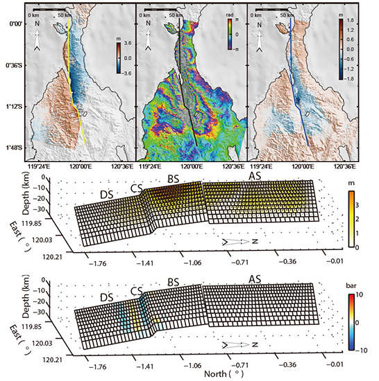
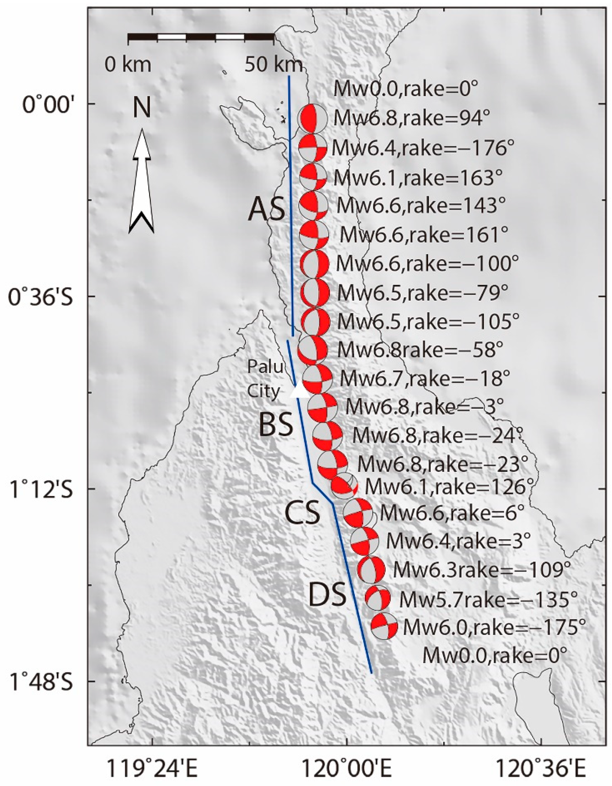
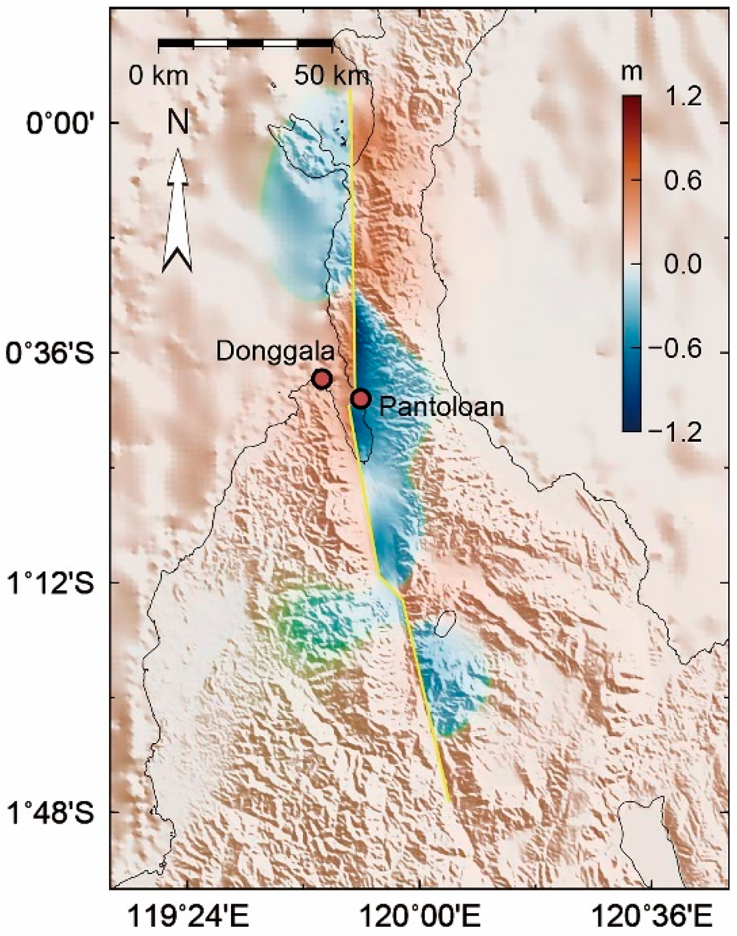
3.1. Slip Model
3.2. CFS Change
4. Discussion
5. Conclusions
Supplementary Materials
Author Contributions
Funding
Acknowledgments
Conflicts of Interest
References
- Watkinson, I.M.; Hall, R. Fault systems of the eastern Indonesian triple junction: Evaluation of Quaternary activity and implications for seismic hazards. Geol. Soc. Lond. Spec. Publ. 2016, 441, SP441.448. [Google Scholar] [CrossRef]
- Bellier, O.; Sébrier, M.; Beaudouin, T.; Villeneuve, M.; Braucher, R.; Bourles, D.; Siame, L.; Putranto, E.; Pratomo, I.J.T.N. High slip rate for a low seismicity along the Palu-Koro active fault in central Sulawesi (Indonesia). Terra Nova 2001, 13, 463–470. [Google Scholar] [CrossRef]
- Socquet, A.; Simons, W.; Vigny, C.; McCaffrey, R.; Subarya, C.; Sarsito, D.; Ambrosius, B.; Spakman, W. Microblock rotations and fault coupling in SE Asia triple junction (Sulawesi, Indonesia) from GPS and earthquake slip vector data. J. Geophys. Res. Solid Earth 2006, 111, 1–15. [Google Scholar] [CrossRef]
- Vigny, C.; Perfettini, H.; Walpersdorf, A.; Lemoine, A.; Simons, W.; Van Loon, D.; Ambrosius, B.; Stevens, C.; McCaffrey, R.; Morgan, P.; et al. Migration of seismicity and earthquake interactions monitored by GPS in SE Asia triple junction: Sulawesi, Indonesia. J. Geophys. Res. Solid Earth 2002, 107, ETG 7-1–ETG 7-11. [Google Scholar] [CrossRef]
- Stevens, C.; McCaffrey, R.; Bock, Y.; Genrich, J.; Subarya, C.; Puntodewo, S.S.O.; Vigny, C. Rapid rotations about a vertical axis in a collisional setting revealed by the Palu fault, Sulawesi, Indonesia. Geophys. Res. Lett. 1999, 26, 2677–2680. [Google Scholar] [CrossRef]
- Syifa, M.; Kadavi, P.R.; Lee, C.W. An Artificial Intelligence Application for Post-Earthquake Damage Mapping in Palu, Central Sulawesi, Indonesia. Sensors 2019, 19, 542. [Google Scholar] [CrossRef]
- Liao, J. Detection of land surface change due to the Wenchuan earthquake using multitemporal advanced land observation satellite-phased array type L-band synthetic aperture radar data. J. Appl. Remote Sens. 2009, 3, 031680. [Google Scholar] [CrossRef]
- Satake, M.; Kobayashi, T.; Uemoto, J.; Umehara, T.; Kojima, S.; Matsuoka, T.; Nadai, A.; Uratsuka, S. Damage estimation of the Great East Japan earthquake with airborne SAR (PI-SAR2) data. In Proceedings of the 2012 IEEE International Geoscience and Remote Sensing Symposium, Munich, Germany, 22–27 July 2012; pp. 1190–1191. [Google Scholar]
- Uemoto, J.; Moriyama, T.; Nadai, A.; Kojima, S.; Umehara, T. Landslide detection based on height and amplitude differences using pre-and post-event airborne X-band SAR data. Nat. Hazards 2019, 95, 485–503. [Google Scholar] [CrossRef]
- Gabriel, A.K.; Goldstein, R.M.; Zebker, H.A. Mapping small elevation changes over large areas: Differential radar interferometry. J. Geophys. Res. Solid Earth 1989, 94, 9183–9191. [Google Scholar] [CrossRef]
- Massonnet, D.; Rossi, M.; Carmona, C.; Adragna, F.; Pelter, G.; Feigl, K.; Rabaute, T. The displacement field of the Landers earthquake mapped by radar interferometry. Nature 1993, 364, 138–142. [Google Scholar] [CrossRef]
- Weston, J.; Ferreira, A.M.G.; Funning, G.J. Global compilation of interferometric synthetic aperture radar earthquake source models: 1. Comparisons with seismic catalogs. J. Geophys. Res. 2011, 116. [Google Scholar] [CrossRef] [Green Version]
- Lasserre, C.; Peltzer, G.; Crampre, F.; Klinger, Y.; Woerd, J.V.d.; Tapponnier, P. Coseismic deformation of the 2001 Mw=7.8 Kokoxili earthquake in Tibet, measured by synthetic aperture radar interferometry. J. Geophys. Res. 2005, 110, B12408. [Google Scholar] [CrossRef]
- Wang, Y.; Zhu, J.; Ou, Z.; Li, Z.; Xing, X. Coseismic slip distribution of 2009 L’Aquila earthquake derived from InSAR and GPS data. J. Cent. South Univ. 2012, 19, 244–251. [Google Scholar] [CrossRef]
- Feng, W.; Tian, Y.; Zhang, Y.; Samsonov, S.; Almeida, R.; Liu, P. A Slip Gap of the 2016Mw 6.6 Muji, Xinjiang, China, Earthquake Inferred from Sentinel-1 TOPS Interferometry. Seismol. Res. Lett. 2017, 88, 1054–1064. [Google Scholar] [CrossRef]
- Funning, G.J.; Parsons, B.; Wrigth, T.J.; Jackson, J.A.; Fielding, E. Surface displacements and source paramenters of the 2003 Bam (Iran) earthquake from Envisat advanced synthetic aperture radar imagery. J. Geophys. Res. 2005, 110. [Google Scholar] [CrossRef]
- Xu, W.; Feng, G.; Meng, L.; Zhang, A.; Ampuero, J.P.; Bürgmann, R.; Fang, L. Transpressional Rupture Cascade of the 2016 Mw 7.8 Kaikoura Earthquake, New Zealand. J. Geophys. Res. Solid Earth 2018, 123, 2396–2409. [Google Scholar] [CrossRef]
- Socquet, A.; Hollingsworth, J.; Pathier, E.; Bouchon, M. Evidence of supershear during the 2018 magnitude 7.5 Palu earthquake from space geodesy. Nat. Geosci. 2019, 12, 192–199. [Google Scholar] [CrossRef]
- Zhang, Y.; Chen, Y.; Feng, W. Complex multiple-segment ruptures of the 28 September 2018, Sulawesi, Indonesia, earthquake. Sci. Bull. 2019, 64, 650–652. [Google Scholar] [CrossRef] [Green Version]
- Bao, H.; Ampuero, J.-P.; Meng, L.; Fielding, E.J.; Liang, C.; Milliner, C.W.D.; Feng, T.; Huang, H. Early and persistent supershear rupture of the 2018 magnitude 7.5 Palu earthquake. Nat. Geosci. 2019, 12, 200–205. [Google Scholar] [CrossRef]
- Fang, J.; Xu, C.; Wen, Y.; Wang, S.; Xu, G.; Zhao, Y.; Yi, L. The 2018 Mw 7.5 Palu Earthquake: A Supershear Rupture Event Constrained by InSAR and Broadband Regional Seismograms. Remote Sens. 2019, 11, 1330. [Google Scholar] [CrossRef]
- Song, X.; Zhang, Y.; Shan, X.; Liu, Y.; Gong, W.; Qu, C. Geodetic Observations of the 2018 Mw 7.5 Sulawesi Earthquake and Its Implications for the Kinematics of the Palu Fault. Geophys. Res. Lett. 2019, 46, 4212–4220. [Google Scholar] [CrossRef]
- Adriano, B.; Xia, J.; Baier, G.; Yokoya, N.; Koshimura, S. Multi-Source Data Fusion Based on Ensemble Learning for Rapid Building Damage Mapping during the 2018 Sulawesi Earthquake and Tsunami in Palu, Indonesia. Remote Sens. 2019, 11, 886. [Google Scholar] [CrossRef]
- Wegmüller, U.; Werner, C. Gamma SAR processor and interferometry software. In Proceedings of the Third ERS Symposium on Space at the service of our Environment, Florence, Italy, 14–21 March 1997; pp. 1686–1692. [Google Scholar]
- Farr, T.G.; Rosen, P.A.; Caro, E.; Crippen, R.; Duren, R.; Hensley, S.; Kobrick, M.; Paller, M.; Rodriguez, E.; Roth, L. The shuttle radar topography mission. Rev. Geophys. 2007, 45. [Google Scholar] [CrossRef]
- Goldstein, R.M.; Werner, C.L. Radar interferogram filtering for geophysical applications. Geophys. Res. Lett. 1998, 25, 4035–4038. [Google Scholar] [CrossRef] [Green Version]
- Costantini, M. A novel phase unwrapping method based on network programming. IEEE Trans. Geosci. Remote Sens. 1998, 36, 813–821. [Google Scholar] [CrossRef]
- Chen, C.W.; Zebker, H.A. Network approaches to two-dimensional phase unwrapping: Intractability and two new algorithms. J. Opt. Soc. Am. A 2000, 17, 401–414. [Google Scholar] [CrossRef]
- Xu, B.; Li, Z.; Wang, Q.; Jiang, M.; Zhu, J.; Ding, X. A Refined Strategy for Removing Composite Errors of SAR Interferogram. IEEE Geosci. Remote Sens. Lett. 2014, 11, 143–147. [Google Scholar] [CrossRef]
- Jónsson, S.; Zebker, H.; Segall, P.; Amelung, F. Fault Slip Distribution of the 1999 Mw7.1 Hector Mine, California Earthquake, Estimated from Satellite Radar and GPS Measurements. Bull. Seism. Soc. Am. 2002, 92, 1377–1389. [Google Scholar] [CrossRef]
- Ou, D.; Tan, K.; Du, Q.; Chen, Y.; Ding, J. Decision Fusion of D-InSAR and Pixel Offset Tracking for Coal Mining Deformation Monitoring. Remote Sens. 2018, 10, 1055. [Google Scholar] [CrossRef]
- Hu, J.; Li, Z.; Zhang, L.; Ding, X.; Zhu, J.; Sun, Q.; Ding, W. Correcting ionospheric effects and monitoring two-dimensional displacement fields with multiple-aperture InSAR technology with application to the Yushu earthquake. Sci. China Earth Sci. 2012, 55, 1961–1971. [Google Scholar] [CrossRef]
- Wang, Y.; Zhu, J.; Li, Z.; Ou, Z. Coseismic slip distribution inversion of the 2011 Yushu earthquake using PALSAR data. Acta Geod. Cartogr. Sin. 2013, 42, 27–33. [Google Scholar]
- Feng, G.; Hetland, E.A.; Ding, X.; Li, Z.; Zhang, L. Coseismic fault slip of the 2008 Mw 7.9 Wenchuan earthquake estimated from InSAR and GPS measurements. Geophys. Res. Lett. 2010, 37. [Google Scholar] [CrossRef]
- Walpersdorf, A.; Vigny, C.; Subarya, C.; Manurung, P. Monitoring of the Palu-Koro Fault (Sulawesi) by GPS. Geophys. Res. Lett. 1998, 25, 2313–2316. [Google Scholar] [CrossRef] [Green Version]
- Zhang, Y.; Wang, R. Geodetic inversion for source mechanism variations with application to the 2008 Mw7. 9 Wenchuan earthquake. Geophys. J. Int. 2015, 200, 1627–1635. [Google Scholar] [CrossRef]
- Okada, Y. Surface Deformation Due to Shear and tensile faults in a half-space. Bull. Seism. Soc. Am. 1985, 75, 1135–1154. [Google Scholar]
- Fialko, Y. Probing the mechanical properties of seismically active crust with space geodesy: Study of the co-seismic deformation due to the 1992 Mw7.3 Landers (southern California) earthquake. J. Geophys. Res. 2004, 109. [Google Scholar] [CrossRef]
- Xu, X.; Tong, X.; Sandwell, D.T.; Milliner, C.W.D.; Dolan, J.F.; Hollingsworth, J.; Leprince, S.; Ayoub, F. Refining the shallow slip deficit. Geophys. J. Int. 2016, 204, 1843–1862. [Google Scholar] [CrossRef]
- Wang, K.; Fialko, Y. Space geodetic observations and models of postseismic deformation due to the 2005 M7.6 Kashmir (Pakistan) earthquake. J. Geophys. Res. Solid Earth 2014. [Google Scholar] [CrossRef]
- Wen, Y.; Xu, C.; Liu, Y.; Jiang, G. Deformation and Source Parameters of the 2015 Mw 6.5 Earthquake in Pishan, Western China, from Sentinel-1A and ALOS-2 Data. Remote Sens. 2016, 8, 134. [Google Scholar] [CrossRef]
- Vajedian, S.; Motagh, M.; Mousavi, Z.; Motaghi, K.; Fielding, E.; Akbari, B.; Wetzel, H.-U.; Darabi, A. Coseismic Deformation Field of the Mw 7.3 12 November 2017 Sarpol-e Zahab (Iran) Earthquake: A Decoupling Horizon in the Northern Zagros Mountains Inferred from InSAR Observations. Remote Sens. 2018, 10, 1589. [Google Scholar] [CrossRef]
- Hodge, M.; Fagereng, Å.; Biggs, J. The Role of Coseismic Coulomb Stress Changes in Shaping the Hard Link Between Normal Fault Segments. J. Geophys. Res. Solid Earth 2018, 123, 797–814. [Google Scholar] [CrossRef] [Green Version]
- Yang, Y.-H.; Hu, J.-C.; Tung, H.; Tsai, M.-C.; Chen, Q.; Xu, Q.; Zhang, Y.-J.; Zhao, J.-J.; Liu, G.-X.; Xiong, J.-N.; et al. Co-Seismic and Postseismic Fault Models of the 2018 Mw 6.4 Hualien Earthquake Occurred in the Junction of Collision and Subduction Boundaries Offshore Eastern Taiwan. Remote Sens. 2018, 10, 1372. [Google Scholar] [CrossRef]
- King, G.C.P.; Stein, R.S.; Lin, J. Static Stress Changes and the Triggering of Earthquakes. Bull. Seism. Soc. Am. 1994, 84, 935–953. [Google Scholar]
- Toda, S. Forecasting the evolution of seismicity in southern California: Animations built on earthquake stress transfer. J. Geophys. Res. 2005, 110. [Google Scholar] [CrossRef]
- Ulrich, T.; Vater, S.; Madden, E.H.; Behrens, J.; van Dinther, Y.; van Zelst, I.; Fielding, E.J.; Liang, C.; Gabriel, A.-A. Coupled, Physics-based Modeling Reveals Earthquake Displacements are Critical to the 2018 Palu, Sulawesi Tsunami. Pure Appl. Geophys. 2019, 1–41. [Google Scholar] [CrossRef]
- Jiang, J.; Lapusta, N. Connecting depth limits of interseismic locking, microseismicity, and large earthquakes in models of long-term fault slip. J. Geophys. Res.: Solid Earth 2017, 122, 6491–6523. [Google Scholar] [CrossRef]
- Jiang, J.; Lapusta, N. Deeper penetration of large earthquakes on seismically quiescent faults. Science 2016, 352, 1293–1297. [Google Scholar] [CrossRef] [Green Version]
- Sassa, S.; Takagawa, T. Liquefied gravity flow-induced tsunami: First evidence and comparison from the 2018 Indonesia Sulawesi earthquake and tsunami disasters. Landslides 2018, 16, 195–200. [Google Scholar] [CrossRef]
- Heidarzadeh, M.; Muhari, A.; Wijanarto, A.B. Insights on the Source of the 28 September 2018 Sulawesi Tsunami, Indonesia Based on Spectral Analyses and Numerical Simulations. Pure Appl. Geophys. 2018, 176, 25–43. [Google Scholar] [CrossRef] [Green Version]
- Omira, R.; Dogan, G.G.; Hidayat, R.; Husrin, S.; Prasetya, G.; Annunziato, A.; Proietti, C.; Probst, P.; Paparo, M.A.; Wronna, M.; et al. The September 28th, 2018, Tsunami in Palu-Sulawesi, Indonesia: A Post-Event Field Survey. Pure Appl. Geophys. 2019, 176, 1379–1395. [Google Scholar] [CrossRef]
- Barnhart, W.D.; Hayes, G.P.; Wald, D.J. Global Earthquake Response with Imaging Geodesy: Recent Examples from the USGS NEIC. Remote Sens. 2019, 11, 1357. [Google Scholar] [CrossRef]
- Hunt, B. A mechanism for tsunami generation. J. Hydraul. Res. 2010, 31, 111–120. [Google Scholar] [CrossRef]
- Kreemer, C.; Holt, W.E.; Goes, S.; Govers, R. Active deformation in eastern Indonesia and the Philippines from GPS and seismicity data. J. Geophys Res. Solid Earth 2000, 105, 663–680. [Google Scholar] [CrossRef]
- Geist, E.L.; Oglesby, D.D. Earthquake Mechanism and Seafloor Deformation for Tsunami Generation. In Encyclopedia of Earthquake Engineering; Beer, M., Kougioumtzoglou, I.A., Patelli, E., Au, I.S.-K., Eds.; Springer Berlin Heidelberg: Berlin, Germany, 2014; pp. 1–17. [Google Scholar] [CrossRef]
- Bie, L.; González, P.J.; Rietbrock, A. Slip distribution of the 2015 Lefkada earthquake and its implications for fault segmentation. Geophys. J. Int. 2017, 210, 420–427. [Google Scholar] [CrossRef]
- Harris, R.A.; Day, S.M. Dynamics of fault interaction: Parallel strike-slip faults. J.Geophys. Res. Solid Earth 1993, 98, 4461–4472. [Google Scholar] [CrossRef]
- Harris, R.A.; Day, S.M. Dynamic 3D simulations of earthquakes on En Echelon Faults. Geophys. Res. Lett. 1999, 26, 2089–2092. [Google Scholar] [CrossRef]
- Li, Z.; Zhou, B. Influence of fault steps on rupture termination of strike-slip earthquake faults. J. Seismol. 2017, 22, 487–498. [Google Scholar] [CrossRef]
- Wei, S.; Feng, G.; Zeng, H.; Martin, S.; Shi, Q.; Muzli, M.; Wang, T.; Lindsey, E.; Triyono, R.; Hubbard, J.; et al. The 2018 Mw 7.5 Palu Earthquake, a Gradually Accelerating Super-Shear Rupture Stopped by Stress Shadows in a Complex Fault System; AGU Fall Meeting Abstracts: Washington, DC, USA, 2018. [Google Scholar]
- Wessel, P.; Smith, W.H.F. New, improved version of generic mapping tools released. EOS Trans. AGU 1998, 79, 579. [Google Scholar] [CrossRef]


| Path Number | Acquisition Time (M-D-Y) | Heading Angle (°) | Incidence Angle (°) |
|---|---|---|---|
| 25 | 09-27-2018 | 195 | 39 |
| 10-11-2018 | |||
| 26 | 08-21-2018 | 195 | 39 |
| 10-02-2018 |
| Segment Name | Top Center Lon | Top Center Lat | Strike | Dip | Length | Width |
|---|---|---|---|---|---|---|
| ° | ° | ° | ° | km | Km | |
| AS | 119.8278 | −0.3187 | 359.14 | 67 | 90 | 20 |
| BS | 119.8558 | −0.9587 | 349.98 | 67 | 50 | 20 |
| CS | 119.9258 | −1.2140 | 316.72 | 67 | 10 | 20 |
| DS | 120.0171 | −1.5109 | 347.11 | 67 | 60 | 20 |
© 2019 by the authors. Licensee MDPI, Basel, Switzerland. This article is an open access article distributed under the terms and conditions of the Creative Commons Attribution (CC BY) license (http://creativecommons.org/licenses/by/4.0/).
Share and Cite
Wang, Y.; Feng, W.; Chen, K.; Samsonov, S. Source Characteristics of the 28 September 2018 Mw 7.4 Palu, Indonesia, Earthquake Derived from the Advanced Land Observation Satellite 2 Data. Remote Sens. 2019, 11, 1999. https://doi.org/10.3390/rs11171999
Wang Y, Feng W, Chen K, Samsonov S. Source Characteristics of the 28 September 2018 Mw 7.4 Palu, Indonesia, Earthquake Derived from the Advanced Land Observation Satellite 2 Data. Remote Sensing. 2019; 11(17):1999. https://doi.org/10.3390/rs11171999
Chicago/Turabian StyleWang, Yongzhe, Wanpeng Feng, Kun Chen, and Sergey Samsonov. 2019. "Source Characteristics of the 28 September 2018 Mw 7.4 Palu, Indonesia, Earthquake Derived from the Advanced Land Observation Satellite 2 Data" Remote Sensing 11, no. 17: 1999. https://doi.org/10.3390/rs11171999