Scale Accuracy Evaluation of Image-Based 3D Reconstruction Strategies Using Laser Photogrammetry

Abstract

Rapid developments in the field of underwater photogrammetry have given scientists the ability to produce accurate 3-dimensional (3D) models which are now increasingly used in the representation and study of local areas of interest. This paper addresses the lack of systematic analysis of 3D reconstruction and navigation fusion strategies, as well as associated error evaluation of models produced at larger scales in GPS-denied environments using a monocular camera (often in deep sea scenarios). Based on our prior work on automatic scale estimation of Structure from Motion (SfM)-based 3D models using laser scalers, an automatic scale accuracy framework is presented. The confidence level for each of the scale error estimates is independently assessed through the propagation of the uncertainties associated with image features and laser spot detections using a Monte Carlo simulation. The number of iterations used in the simulation was validated through the analysis of the final estimate behavior. To facilitate the detection and uncertainty estimation of even greatly attenuated laser beams, an automatic laser spot detection method was developed, with the main novelty of estimating the uncertainties based on the recovered characteristic shapes of laser spots with radially decreasing intensities. The effects of four different reconstruction strategies resulting from the combinations of Incremental/Global SfM, and the a priori and a posteriori use of navigation data were analyzed using two distinct survey scenarios captured during the SUBSAINTES 2017 cruise (doi: 10.17600/17001000). The study demonstrates that surveys with multiple overlaps of nonsequential images result in a nearly identical solution regardless of the strategy (SfM or navigation fusion), while surveys with weakly connected sequentially acquired images are prone to produce broad-scale deformation (doming effect) when navigation is not included in the optimization. Thus the scenarios with complex survey patterns substantially benefit from using multiobjective BA navigation fusion. The errors in models, produced by the most appropriate strategy, were estimated at around $1\%$ in the central parts and always inferior to $5\%$ on the extremities. The effects of combining data from multiple surveys were also evaluated. The introduction of additional vectors in the optimization of multisurvey problems successfully accounted for offset changes present in the underwater USBL-based navigation data, and thus minimize the effect of contradicting navigation priors. Our results also illustrate the importance of collecting a multitude of evaluation data at different locations and moments during the survey.

1. Introduction

Accurate and detailed 3D models of the environment are now an essential tool in different scientific and applied fields, such as geology, biology, engineering, archaeology, among others. With advancements in photographic equipment and improvements in image processing and computational capabilities of computers, optical cameras are now widely used due to their low cost, ease of use, and sufficient accuracy of the resulting models for their scientific exploitation. The application of traditional aerial and terrestrial photogrammetry has greatly expanded in recent years, with commercial and custom-build camera systems and software solutions enabling a nearly black-box type of data processing (e.g., the works by the authors of [1,2,3,4]).

These rapid developments have also significantly benefited the field of underwater photogrammetry. The ability to produce accurate 3D models from monocular cameras under unfavorable properties of the water medium (i.e., light attenuation and scattering, among other effects) [5], and advancements of unmanned underwater vehicles have given scientists unprecedented access to image the seafloor and its ecosystems from shallow waters to the deep ocean [6,7,8,9]. Optical seafloor imagery is now routinely acquired with deep sea vehicles, and often associated with other geophysical data (acoustic backscatter and multibeam bathymetry) and water column measurements (temperature, salinity, and chemical composition). High-resolution 3D models with associated textures are, thus, increasingly used in the representation and study of local areas of interest. However, most remotely operated vehicles (ROVs) or autonomous underwater vehicles (AUVs) that are currently used in science missions have limited optical sensing capabilities, commonly comprising a main camera used by the ROV-pilot, while larger workclass ROVs have additional cameras for maneuvering. Due to the nature of projective geometry, performing 3D reconstruction using only optical imagery acquired by monocular cameras results in a 3D model which is defined only up to scale, meaning that the unit in the model is not necessary a standard unit such as a meter [10]. In order to correctly disambiguate the scale, it is essential to use additional information in the process of model building. Predominantly, solutions in subaerial applications are based on the fusion of image measurement with robust and dependable satellite references, such as Global Navigation Satellite System (GNSS) [11,12,13], or ground control pointss (GCPs) [14,15,16], due to their accuracy and ease of integration. On the contrary, the water medium not only hinders the possibility of accurately establishing the control points, but also prevents the use of global positioning system (GPS) due to the absorption of electromagnetic waves. Hence the scale is normally disambiguated either using a combination of acoustic positioning (e.g., Ultra-Short BaseLine (USBL)) and inertial navigation system (INS) [17,18,19], or through the introduction of known distances between points in the scene [20].

In shallow water environments, i.e., accessible by divers, researchers have often placed auxiliary objects (such as a scaling cube [21], locknuts [22], graduated bars [23], etc.) into the scene, and used the knowledge of their dimensions to scale the model a posteriori. Such approaches, while applicable in certain scenarios, are limited to the use in small-scale reconstructions (e.g., a few tens of square meters), and in shallow water environments, due to the challenges in transporting and placing objects in deep sea environments. Similarly, laser scalers have been used since the late 1980s, projecting parallel laser beams onto the scene to estimate the scale of the observed area, given the known geometric setup of the lasers. Until recently, lasers have been mostly used in image-scaling methods, for measurements within individual images (e.g., Pilgrim et al. [24] and Davis and Tusting [25]). To provide proper scaling, we have recently proposed two novel approaches [26], namely, a fully-unconstrained (FUM) and a partially-constrained method (PCM), to automatically estimate 3D model scale using a single optical image with identifiable laser projections. The proposed methods alleviate numerous restrictions imposed by earlier laser photogrammetry methods (e.g., laser alignment with the optical axis of the camera, perpendicularity of lasers with the scene), and remove the need for manual identification of identical points on the image and 3D model. The main drawback of these methods is the need for purposeful acquisition of images with laser projections, with the required additional acquisition time.

Alternatively, the model scaling can be disambiguated with known metric vehicle displacements (i.e., position and orientation from acoustic positioning, Doppler systems, and depth sensors [19,27,28]). As this information is recorded throughout the mission, such data are normally available for arbitrary segments even if they have not been identified as interesting beforehand. The classic range-and-bearing position estimates from acoustic-based navigation, such as USBL, have an uncertainty that increases with increasing range (i.e., depth) in addition to possible loss of communication (navigation gaps). Consequently, the scale information is inferred from data which is often noisy, poorly resolved, or both. Hence the quality of the final dataset is contingent on the strategy used in the fusion of image and navigation information. Depending on the approach, the relative ambiguity can cause scale drift, i.e., a variation of scale along the model, causing distortions [29]. Furthermore, building of large 3D models may require fusion of imagery acquired in multiple surveys. This merging often results in conflicting information from different dives, and affects preferentially areas of overlap between surveys, negatively impacting the measurements on the model (distances, areas, angles).

The need to validate the accuracy of image-based 3D models has soared as the development of both the hardware and the techniques enabled the use of standard imaging systems as a viable alternative to more complex and dedicated reconstruction techniques (e.g., structured light). Numerous evaluations of this accuracy are available for aerial and terrestrial 3D models (e.g., the works by the authors of [2,30,31,32]). Environmental conditions and limitations of underwater image acquisition preclude their transposition to underwater image acquisition and, to date, most underwater accuracy studies use known 3D models providing reference measurements. This leads to marine scientists nowadays being constantly faced with the dilemma of selecting appropriate analyses that could potentially be performed on the data derived from the reconstructed 3D models.

Early studies [21,33,34,35,36,37,38] evaluated the accuracy of small-scale reconstructions (mainly on coral colonies), comparing model-based and laboratory-based volume and surface areas for specific corals. More recently, auxiliary objects (e.g., locknuts [22], graduated bars [23], special frames [39,40], and diver weights [41]) have been used to avoid removal of objects from the environment. Reported inaccuracies range from $0.85\%$ to $17\%$, while more recent methods achieve errors as low as 2–$3\%$ [22,41]. Diver-based measurements and the placement of multiple objects at the seafloor both restrict the use of these methods in shallow water or experimental environments, and hinder such approaches in deep sea environments (e.g., scientific cruises), where reference-less evaluation is needed instead, which has been performed in only a few experiments.

Ferrari et al. [38] evaluated their reconstruction method on a medium-size reef area ($400\mathrm{m}$) and a $2\mathrm{k}\mathrm{m}$ long reef transect. Maximum heights of several quadrants within the model were compared to in situ measurements, coupled with an estimation of structural complexity (rugosity). The stated inaccuracies in reef height were $18\pm 2\%$. This study split larger transects into approx $10\mathrm{m}$ long sections to reduce potential drift, and hence model distortion. Similarly, Gonzales et al. [42] reported $15\%$ error in rugosity estimates from stereo imaging and compared them with results from a standard chain-tape method, along a $2\mathrm{k}\mathrm{m}$ long transect. To the best of our knowledge, no other scale accuracy estimate of submarine large-area models has been published. Furthermore, although laser scalers are often used for qualitative visual scaling, they have never been used to evaluate the accuracy of underwater 3D models.

Objectives

Although a growing body of literature supports the belief that underwater image-based 3D reconstruction is a highly efficient and accurate method at small spatial extents, there is a clear absence of scale accuracy analyses of models produced at larger scales (often in deep sea scenarios). Validation of 3D reconstruction methods and associated error evaluation are, thus, required for large underwater scenes and to allow the quantitative measurements (distances and volumes, orientations, etc.) required for scientific and technical studies.

The main goal of this paper is to present and use an automatic scale accuracy estimation framework, applicable to models reconstructed from optical imagery and associated navigation data. We evaluate various reconstruction strategies, often used in research and industrial ROV deep sea surveys.

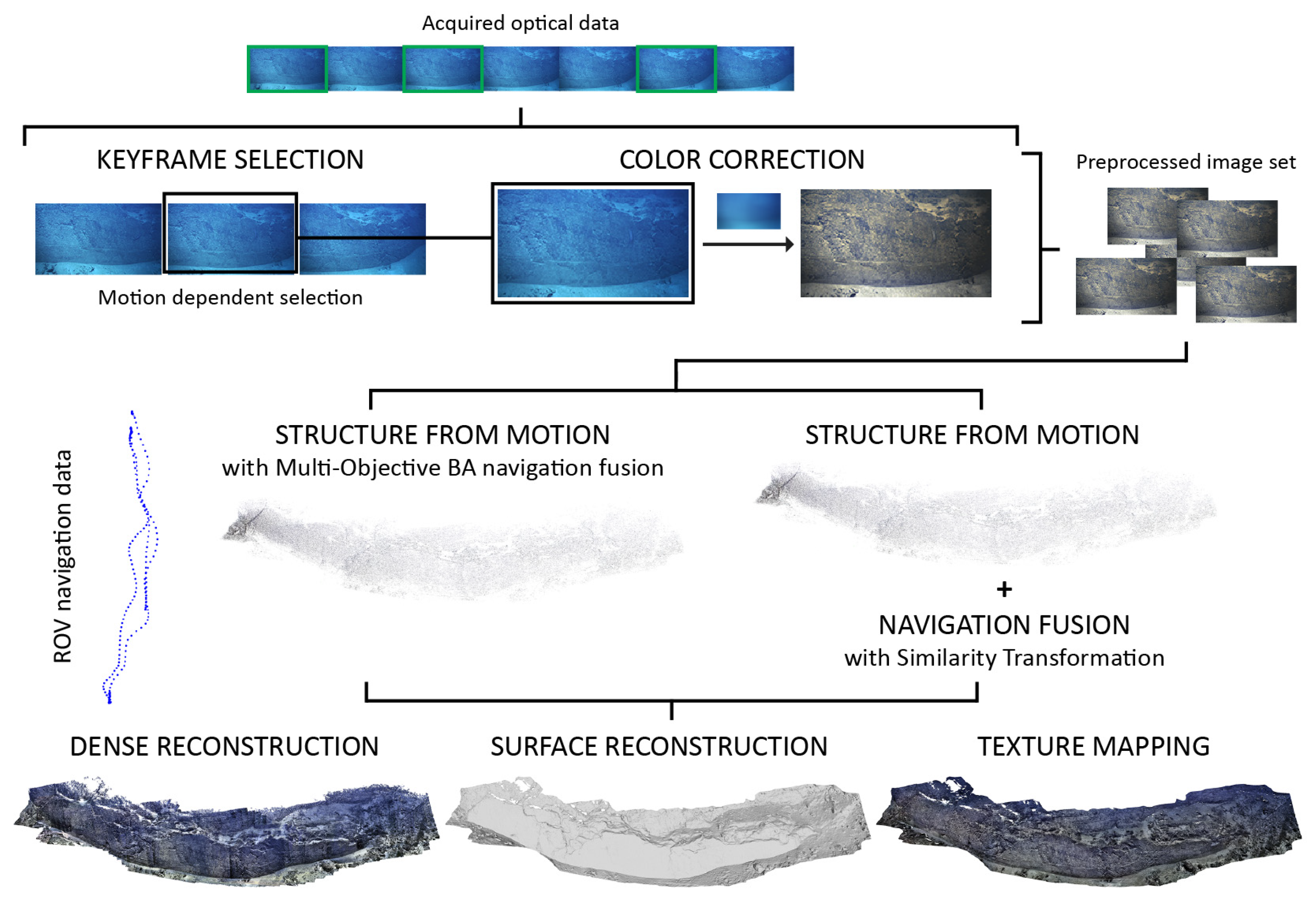
First, we present several methods of 3D reconstruction using underwater vehicle navigation, to provide both scaling and an absolute geographic reference. Most commonly, SfM uses either an incremental or a global strategy, while the vehicle navigation may be considered a priori as part of the optimization process, or a posteriori after full 3D model construction. Here, we compare four different strategies resulting from combination of Incremental/Global SfM and the a priori and a posteriori use of navigation data. We discuss the impact of each strategy in the final 3D model accuracy.

Second, the four methods are evaluated to identify which one is best suited to generate 3D models that combine data from multiple surveys, as this is often required under certain surveying scenarios. Navigation data from different surveys may have significant offsets at the same location (x, y, z, rotation), show noise differences, or both. The changes between different acquisitions of a single scene are taken into account differently by each 3D reconstruction strategy.

Third, prior approaches, recently presented by Istenič et al. [26], to estimating model scale using laser scalers, namely FUM and PCM methods, are augmented with Monte Carlo simulations to evaluate the uncertainty of the obtained scale estimates. Furthermore, the results are compared to the kinds of estimates commonly used and suffering from parallax error.

Fourth, an automatic laser detection and uncertainty estimation method is presented. Accurate analyses require a multitude of reliable measurements spread across the 3D model, whose manual annotation is extremely labor-intensive, error-prone, and time-consuming, when not nearly impossible. Unlike previous detection methods, our method detects the centers of laser beams by considering the texture of the scene, and then determines their uncertainty, which, to the best of our knowledge, has not been presented in the literature hitherto.

With the data from the SUBSAINTES 2017 cruise (doi: 10.17600/17001000; [43]) we evaluate the advantages and drawbacks of the different strategies to construct underwater 3D models, while providing quantitative error estimates. As indicated above, these methods are universal as they are not linked to data acquired using specific sensors (e.g., laser systems and stereo cameras), and can be applied to standard imagery acquired with underwater ROVs. Hence, it is possible to process legacy data from prior cruises and with different vehicles and/or imaging systems. Finally, we discuss the best practices for conducting optical surveys, based on the nature of targets and the characteristics of the underwater vehicle and sensors.

2. Image-Based Underwater 3D Reconstruction

Textured 3D models result from a set of sequential processing steps (Figure 1). As scene geometry is computed entirely from the optical imagery, the end result directly depends on image quality and an adequate survey strategy. Compared to subaerial imagery, the unfavorable properties of the water medium (i.e., light attenuation and scattering effects) [5] cause blurring of details, low image contrast, and distance-dependent color shifts [44]. As such, acquisition is conducted at close range, thus limiting the observation area of any single image, while significantly increasing the amount of data collected and processed. The distance from the camera to the scene is often defined by a combination of several factors, such as the visibility, amount of available light, terrain roughness, and maneuverability of the imaging platform. As some of these factors may change from place to place and over time; it is common to adjust the distance during acquisition. The survey speed is also affected by several factors. Commonly, the survey speed is adjusted as a function of the distance to the scene and of the image exposure time, in order to keep motion blurriness to minimum levels (often less than 2 pixels). Typically, the survey speed is in the order of a $1/4$ of the distance to the scene, per second.

2.1. Preprocessing

Keyframe selection is hence important preprocessing step, used to remove unnecessary redundancy (i.e., images taken from very similar poses). Selecting too many images may represent an unnecessary increase of processing time, whereas the selection of too few images may result in missing observations and prevent the reconstruction of a single complete model. The commonly used strategy for image selection based on constant time intervals (e.g., selecting a frame every n-th second) is often not suitable; surveys with significant changes in speed and/or distance to the scene can lead to over- or underselection of images. Instead, we use an approach with implicit detection of frames with similar vantage points [45] through estimates of feature displacements between consecutive frames (e.g., Lucas–Kanade tracking algorithm [46]). For sufficiently dense image sets (e.g., video acquisitions), sharpness may be used for further selection (e.g., variance of Laplacian [47]).

Additionally, color correction can be used to counteract the degradation effects of water. Minimizing the effects of the water medium not only benefits human perception and interpretation of the scene, but also improves the quality and quantity of successful feature matches between image pairs [48], thus increasing the quality of the final model. Accurate color information recovery depends on knowledge of the physical image formulation process model which is rarely available in its completeness. Alternatively, color enhancing methods (e.g., Bianco et al. [49] used in our tests) can remove the attenuation effects, as well as the color cast introduced by an unknown illuminant (Figure 2).

2.2. Sparse Reconstruction

A concise set of preselected images is then used to jointly estimate the sparse 3D geometry of the scene (set of 3D points) and the motion of the camera (trajectory) through a technique called Structure from Motion (SfM). The inherent scale ambiguity of the reconstructed 3D structure and camera motion from a set of images taken by a monocular camera is addressed by either using the vehicle navigation a priori as part of the optimization process (multiobjective BA), or a posteriori through an alignment with the reconstructed camera path using a similarity transformation.

As the structure and motion parameters are inferred entirely from multiple projections of the same 3D point in overlapping images, the robustness of detection, and matching of feature points across the image set is important. In the evaluated approach, the features are detected as accelerated KAZE (AKAZE) [50], and described using Modified-SURF descriptors [51]. To avoid an empirical selection of the inlier/outlier threshold in the geometric filtering procedure (e.g., fundamental/essential matrix [10]), a parameter-free A Contrario Ransac (AC-RANSAC) [52], implemented in openMVG library [53], is used. The approach automatically determines the threshold and model meaningfulness by a statistical balance between the tightness of fitting of data and the number of the inliers.

Due to the nonlinearity in the projection process, a nonlinear optimization, Bundle Adjustment (BA), is required, with the final solution obtained by formulating a nonlinear least squares (NLS) problem. The cost function to be minimized is normally an image-based error, consisting of the sum of squared re-projection errors, defined as the distances between the 2-dimensional (2D) feature observations of the 3D point and their corresponding projections onto the images. Intrinsic camera parameters, if a priori known, can be excluded from the optimization, leading to lowering the complexity of the problem and thus improving the results. The problem can be efficiently solved using iterative methods such as Levenberg-Marquardt (LM) [54], which, however, only guarantees finding a local minimum of the optimizing function. This makes it extremely sensitive to the initial parameter estimate, leading to different strategies proposed for their initialization broadly classified as either: incremental or global.

Incremental SfM expands model reconstruction one image at a time, allowing for a gradual estimation of parameters for the newly added points and cameras. After each addition, intermediate BA can be performed to propagate and minimize the error of intermediate reconstructions. Incremental approaches are widely used, given that the intermediate partial reconstructions enable a more robust detection of outliers, and thus decrease the chance of convergence to a wrong local minimum. However, when no prior information about the scene is available, the initialization step of decomposing the fundamental/essential matrix is critical, as a poor selection of the seed pair of images can quickly force the optimization to a nonrecoverable state. Furthermore, as the method inherently gives disproportionate weight to images used at the beginning of the process, it can result in error accumulation. This may produce significant drift and fail to reconstruct the scene in the form of a single connected model. In our tests, the method of Moulon et al. [53,55] was used with a contrario model estimation.

Global SfM considers instead the entire problem at once, with full BA performed only at the end. To alleviate the lack of partial reconstructions, that identifies possible outliers, the parameter initialization is split into two sequential steps (i.e., rotation and translation estimation), the first one being more robust to a small number of outliers. This mitigates the need for intermediate nonlinear optimizations, as camera and scene points are estimated simultaneously in a single iteration. It also ensures an equal treatment of all the images, and, consequently, equal distribution of errors. These methods rely on averaging relative rotations and translations, thus requiring images to have overlap with multiple other images, to ensure meaningful constraints and mutual information. As a consequence, the reconstruction from a sparsely connected set of images will result in distorted or even multiple disconnected components. In our test, the method of Moulon et al. [53,56] is used.

2.3. Navigation Fusion

The result of the sparse reconstruction process is thus expressed as a set of 3D points $\mathcal{X}=\{X_k\in {\mathbb{R}}^3\mid k=1\dots L\}$; camera motion is defined with the following set of projection matrices, $\mathcal{P}=\{P_i=\left[{\mathit{R}}_i^T\mid -{\mathit{R}}_i^T{\mathit{t}}_i\right]\mid i=1\dots N\}$, where $P_i\in \mathbf{SE}\left(\mathbf{3}\right)$ defines the projection from world to camera frame, and the following set of intrinsic camera parameters, $\mathcal{K}=\{K_i\mid i=1\dots N\}$. As the joint parameter estimation is an inherently ill-conditioned problem, when estimated from a set of images acquired by a single camera, the solution is determined only up to an unknown scale [10]. The estimated parameters can be multiplied by an arbitrary factor, resulting in an equal projection of the structure on the images. A metric solution thus requires known measurements [20] or metric vehicle displacements (navigation/inertial priors) [19,27,28]. Depending on the availability of synchronization between the camera and the navigation, priors $\mathcal{C}=\{C_i\mid i=1\dots N\}$ extracted from the ROV/AUV’s navigation, can either be used in a multisensor fusion approach or to align the reconstructed camera path via a similarity transformation.

2.3.1. Multiobjective BA

When navigation priors are available for a significant proportion of images, then this information can be incorporated in the optimization through a multisensor fusion approach. When the measurement noises are not known, the problem of appropriate weighting of different objectives arises, as each of the sensor mean squared error (MSE) does not share the same unit neither the same significance [57].

Most commonly, there is no unique solution that would simultaneously optimize both the re-projection (${\displaystyle {\mathcal{E}}_{i,k\left(v\right)}=\parallel x_{i,k}-\mathrm{proj}(K_i,P_i,{\mathit{X}}_k){\parallel }^2}$) and navigation fit errors (${\mathcal{E}}_{i\left(n\right)}=T_i-C_i$). Instead there exists a hypersurface of Pareto optimal solutions, where one of the objective functions can only be improved by degrading the other [58]. Such solution space can be defined as a weighted compound function of the two objectives [57]. Assuming that both re-projection and navigation fit errors are independent and Gaussian, it is statistically optimal to weight the errors by their variance [59,60]:

$${\displaystyle \mathcal{E}=\frac{1}{M{\sigma }_v^2}\sum _{i,k}^{}\parallel {\mathcal{E}}_{i,k\left(v\right)}{\parallel }^2+\frac{1}{N{\sigma }_n^2}\sum _i^{}\parallel {\mathcal{E}}_{i\left(n\right)}{\parallel }^2,}$$

(1)

which can be rewritten as

$${\displaystyle \mathcal{E}=\frac{1}{M}\sum _{i,k}^{}\parallel {\mathcal{E}}_{i,k\left(v\right)}{\parallel }^2+\frac{1}{N}{\lambda }^2\sum _i^{}\parallel {\mathcal{E}}_{i\left(n\right)}{\parallel }^2,}$$

(2)

where $\lambda ={\sigma }_v/{\sigma }_n$ indicates the ratio between the two covariances, representing the noise variance of each sensor measurement and M and N are the number of re-projection and navigation prior terms.

In such cases, the weighting can be selected empirically or through automatic weight-determining methods. For bi-objective optimizations, Michot et al. [57] have shown that the L-Curve criterion is the preferred selection method. This criterion is based on plotting the trade-off between the cost of the objectives using different weights, represented in log–log space. This plot has a typical L-curve shape, with two prominent segments. Each term dominating a segment (flat and vertical part) is used to detect the “corner” separating the two, essentially identifying a neutral objective dominance. The associated weight is considered to be the optimal, and representative of the ratio between the covariances of the sensors. Lying between two nearly flat segments, it can be easily identified as the point with maximum curvature.

2.3.2. Similarity Transformation

Alternatively, the navigation data can be used in an a posteriori step of rescaling and georeferencing. A similarity transformation, which minimizes the sum of differences between the reconstructed camera poses and their navigation priors, is applied to the reconstructed model. Depending on the survey pattern, this method can be used even in cases when the camera is not synchronized with the navigation data. If the reconstructed path can be unambiguously matched to the path given by the navigation data, then the associations between the cameras and navigation poses can be determined through finding the closest points between the paths.

2.4. Dense, Surface and Texture Reconstruction

To better describe the scene geometry, a denser point cloud representation is computed using the method of Shen [61]. For each image reconstructed in SfM, a depth-map is computed, and subsequently refined to enforce consistency over neighboring views. These depth maps are merged into a single (dense) set of 3D points, where points with high photometric inconsistencies are removed to ensure the visibility constraints.

The final steps towards obtaining a final photo-realistic 3D model require estimating both a surface and high-quality texture to be pasted upon such surface. As underwater reconstructions are inevitably affected by noise and outliers [5], a method is used [62] to compute the most probable surface, by modeling the surface as an interface between the free and full space as opposed to directly using the input points. The reconstruction is completed by estimating the texture with a two step method [63]. The method prioritizes near, well-focused and orthogonal high-resolution views, as well as similar adjacent patches. Texture inconsistencies are mitigated by an additional photo-consistency check. Finally, any significant color discontinuities between neighboring regions are addressed by per-vertex-based globally optimal luminance correction as well as with Poisson image editing [64].

3. Model Evaluation Framework

Estimating the scale accuracy of 3D models reconstructed from underwater optical imagery and robot navigation data is of paramount importance since the input data is often noisy and erroneous. The noisy data commonly leads to inaccurate scale estimates and noticeable variations of scale within the model itself, which precludes use of such models for their intended research applications. Real underwater scenarios usually lack elements of known sizes that could be readily used as size references to evaluate the accuracy of 3D models. However, laser scalers are frequently used during underwater image collection to project laser beams onto the scene and can be used to provide such size reference.

The framework we will describe builds upon two recently introduced methods [26] for scale estimation of SfM-based 3D models using laser scalers. We extend the scale estimation process by including it into a Monte Carlo (MC) simulation, where we propagate the uncertainties associated with the image features and laser spot detections through the estimation process.

As the evaluated models are built with metric information (e.g., the vehicle navigation data, dimensions of auxiliary objects), their scale is expected to be consistent with the scale provided by the laser scaler ($s_L$). Therefore, any deviation from the expected scale value ($s=1.0$) can be regarded as an inaccuracy of the scale of the model (${ϵ}_s$). The error can be used to represent the percentage by which any spatial measurement using the model will be affected:

$${ϵ}_s=s_L-1.0=\frac{m}{\widehat{m}}-1.0,$$

(3)

where m and $\widehat{m}$ represent a known metric quantity and its model based estimate.

3.1. Scale Estimation

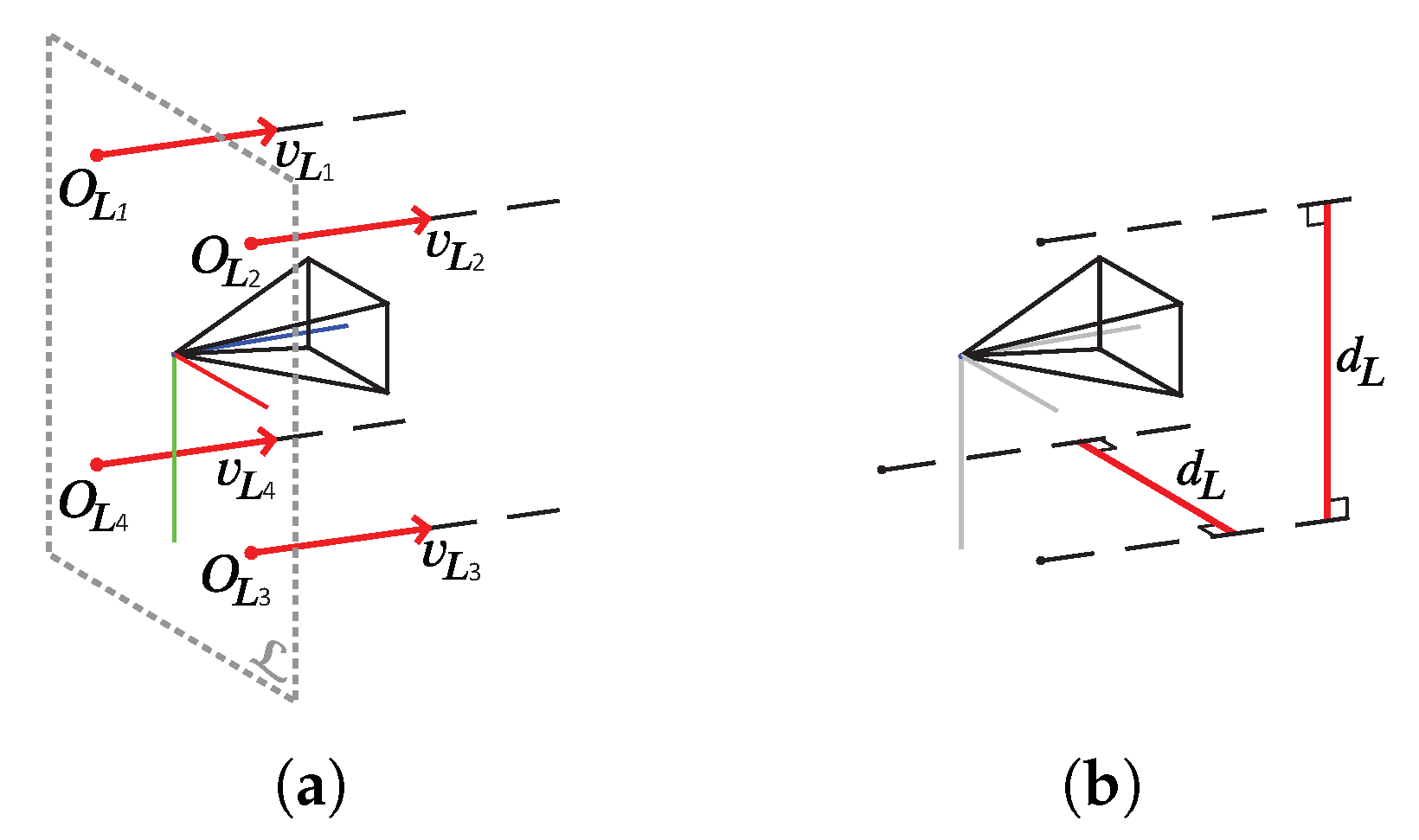
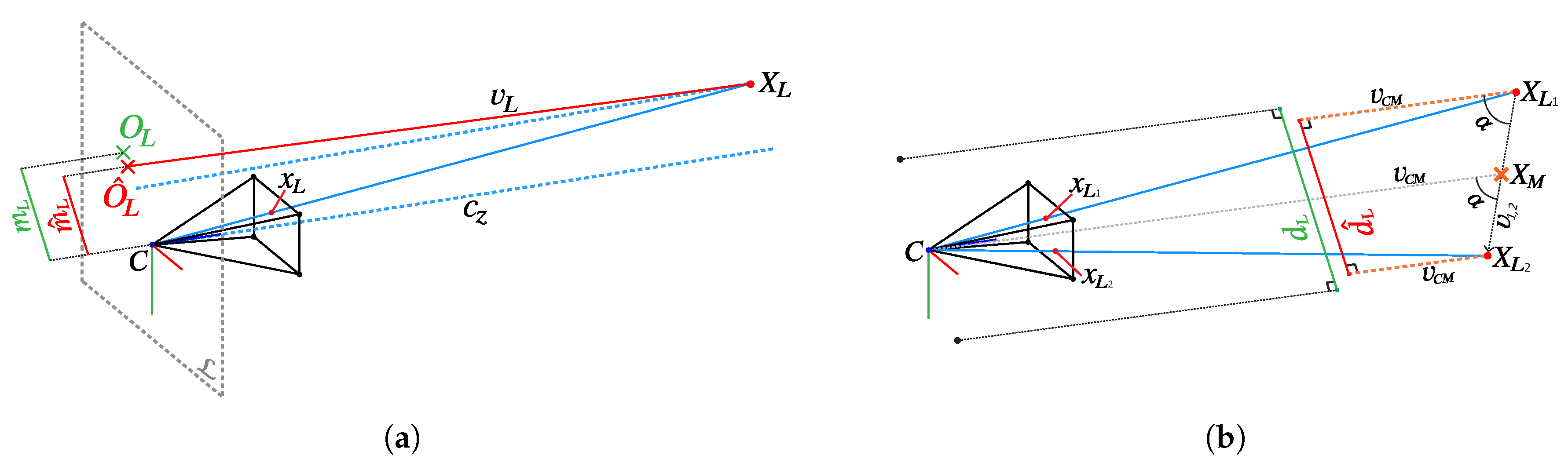
The two methods, namely, the fully-unconstrained method (FUM) and the partially-constrained method (PCM), are both suitable for different laser scaler configurations. FUM permits an arbitrary position and orientation for each of the lasers in the laser scaler, at the expense of requiring a full a priori knowledge of their geometry relative to the camera (Figure 3a). On the other hand, the laser-camera constraints are significantly reduced when using the PCM method. The laser origins have to be equidistant from the camera center and laser pairs have to be parallel (Figure 3b). However, in contrast to prior image scaling methods [24,25], the lasers do not have to be aligned with the optical axis of the camera.

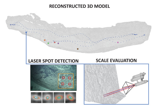
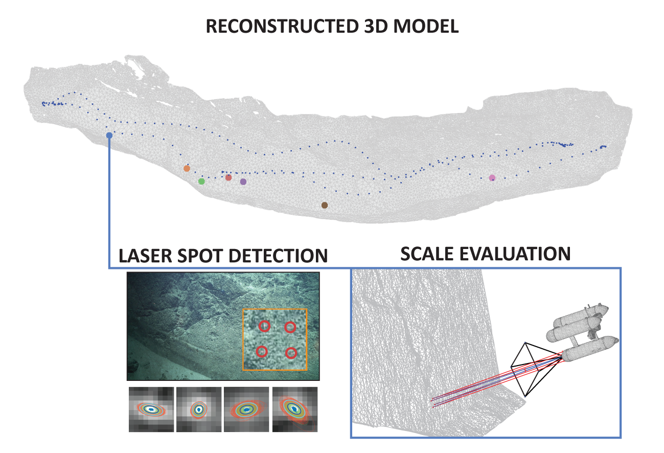
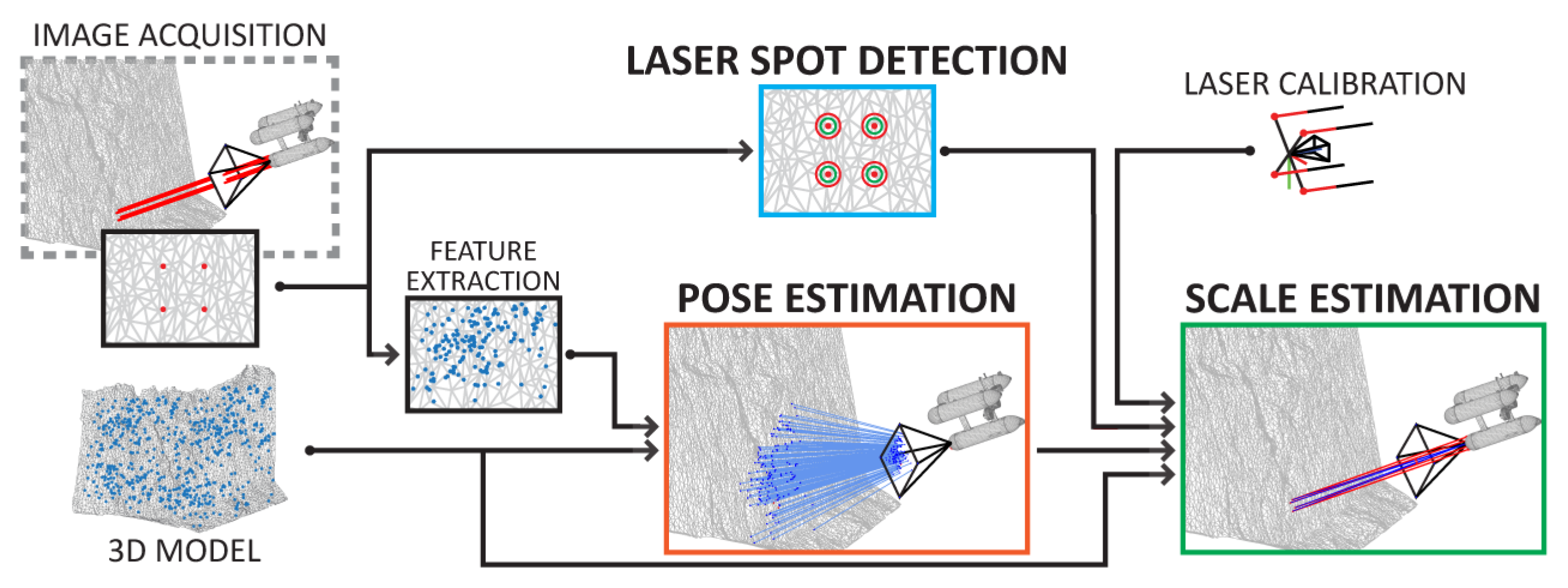
Both methods exploit images with visible intersections of the laser beams with the scene, not just the simple location of the laser spots. The model scale is estimated through a three step process: laser detection, pose estimation and scale estimation (Figure 4). The two initial steps are identical in both methods: First, a laser detection method determines the locations of laser spots on an image; second, the pose of the camera (wrt. the 3D model) at the time of image acquisition is estimated through a feature-based localization process.

The initial camera-extrinsic values (and optionally also camera-intrinsics) are obtained by solving an Perspective-n-Point (PnP) problem [65] using 3D–2D feature pairs. Each pair connects an individual image feature and a feature associated with the sparse set of points representing the model. As these observations and matches are expected to be noisy and can contain outliers, the process is performed in conjunction with a robust estimation method A-Contrario Ransac (AC-RANSAC) [52]. The estimate is further refined through a nonlinear optimization (BA), minimizing the re-projection error of known (and fixed) 3D points and their 2D observation on the image.

The camera pose and location of the laser spots are lastly used either to estimate the position of the laser origin, so as to produce the recorded result (FUM), or else to estimate the perpendicular distance between the two parallel laser beams (PCM). As these predictions are based on the 3D model, they are directly affected by its scale, and can therefore be used to determine it through a comparison with a priori known values. As shown through an extensive evaluation in our previous work, both FUM and PCM can be used to estimate model scale regardless of the camera view angle, camera–scene distance, or terrain roughness [26]. After the application of a maximum likelihood estimator (BA) and a robust estimation method (AC-RANSAC), the final scale estimation is minimally affected by noise in the detection of feature positions and the presence of outlier matches.

In the fully-unconstrained method (Figure 5a), knowledge of the complete laser geometry is used (origins, $O_L$, and directions, $v_L$) to determine the position of laser emission ${\widehat{O}}_L$, and then produce the results observed on the image (Equation (4)). The laser origins ${\widehat{O}}_L$ are predicted by projecting 3D points $X_L$, representing the location of laser beam intersections with the model, using a known direction of the beam $v_L$. As the points $X_L$ must be visible to the camera, i.e., be in the line-of-sight of the camera, their positions can be deduced by a ray-casting procedure using a ray starting in the camera center and passing through the laser spot $x_L$ detected in the image. The final scale estimate can then be determined by comparing the displacement of the ${\widehat{m}}_L=\parallel {\widehat{O}}_L\parallel$ with its a priori known value $\parallel O_L\parallel$.

$${\widehat{O}}_L=\mathit{P}{X}_L-\frac{\mathit{P}{X}_L·c_z}{v_L·c_z}{v}_L,$$

(4)

where $\mathit{P}$ is defined as the projection from world to camera frame and $c_z$ represents the optical axis of the camera.

Alternatively, the partially-constrained method (Figure 5b) can be used when laser pairs are parallel but with unknown relation to the camera. As opposed to other image scaling methods, laser alignment with the optical axis of the camera is not required, allowing its application to numerous scenarios in which strict rigidity between camera and lasers is undetermined or not maintained (e.g., legacy data). To overcome the lack of information on the direction of laser beams with respect to the camera, the equidistance between the laser origins and the camera center is exploited. Laser beam direction is thus approximated with the direction of the vector connecting the camera center and the middle point between the two points of lasers intersections with the model $v_{\mathrm{CM}}$. As we have shown in our previous work [26], this approximation can lead to small scaling errors only in the most extreme cases where the distance discrepancy between two points on the model is disproportionately large compared to the camera–scene distance. As underwater surveys are always conducted at sufficiently large safety distances, this scenario is absent in underwater reconstructions.

3.2. Uncertainty Estimation

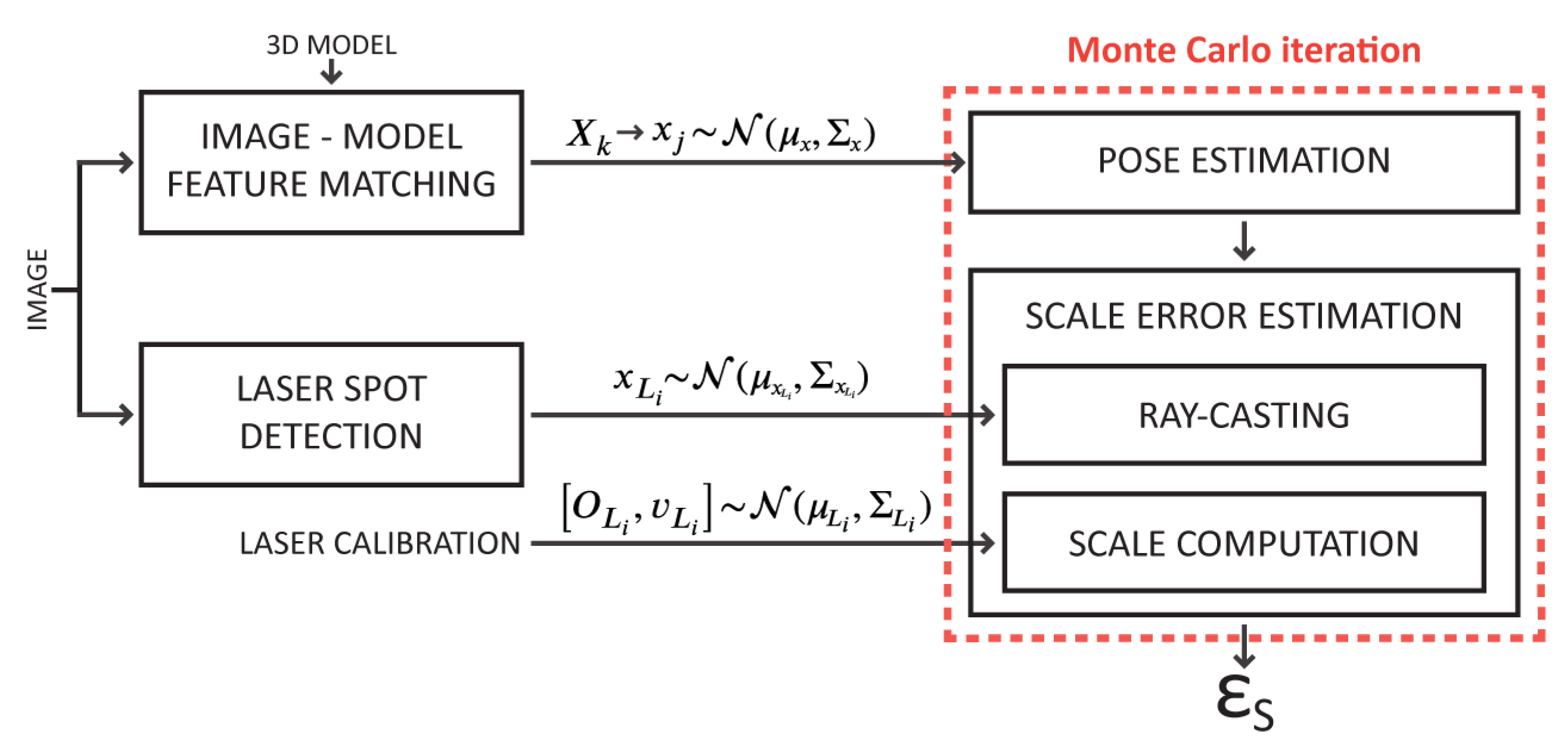
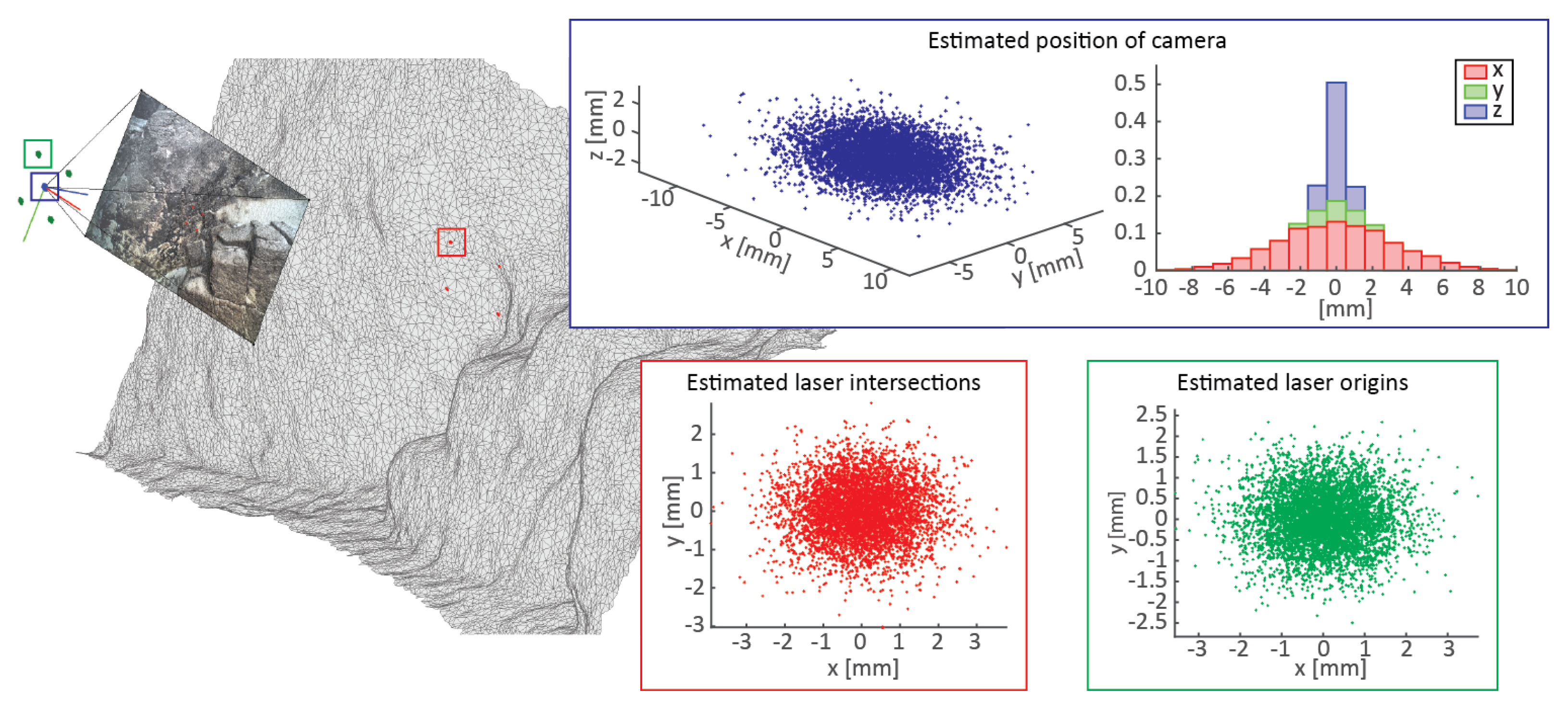
Uncertainty characterization of each scale estimate is crucial for quantitative studies (precise measurement of distances and volumes, orientations, etc.), as required in marine science studies where accurate metrology is essential (such as in geology, biology, engineering, archaeology and others). The effect of uncertainties in the input values on the final estimate is evaluated using a MC simulation method. The propagation of errors through the process is modeled by repeated computations of the same quantities, while statistically sampling the input values based on their probability distributions. The final uncertainty estimate in scale is derived from the independently computed values.

Figure 6 depicts the complete MC simulation designed to compute the probability distribution of an estimated scale error, computed from multiple laser observations in an image. We assume that the sparse 3D model points, associated with the 2D features in the localization process, are constant, and thus noise free. On the other hand, uncertainty in the imaging process and feature detection is characterized using the re-projection error obtained by the localization process. We also account for the plausible uncertainty in the laser calibration and laser spot detection, with each laser being considered independently.

4. Laser Spot Detection

The accurate quantification of scale errors affecting 3D models derived from imagery requires numerous reliable measurements that have to be distributed throughout the model. As scale estimates are obtained by exploiting the knowledge of laser spot positions on the images, the quantity and quality of such detections directly determine the number of useful scale estimates. Furthermore, to properly estimate the confidence levels of such estimated scales, the uncertainty of the laser spot detections needs to be known.

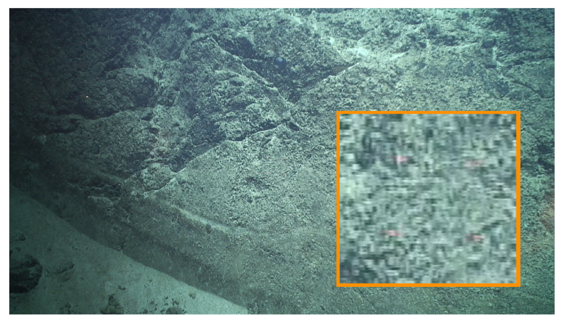
The laser beam center is commonly considered to be the point with the highest intensity in the laser spot, as the luminosity of laser spots normally overpowers the texture of the scene. However, due to the properties of the water medium, the laser light can be significantly attenuated on its path to the surface before being reflected back to the camera. In such cases, the final intensity of the beam reaching the camera might be overly influenced by the texture at the point of the impact (Figure 7). As such, performing manual accurate annotations of laser spots tends to be extremely challenging and labor intensive, and even impossible in certain cases.

Considerable attention has been given to the development of the image processing components of laser scanners, namely on laser line detection [66,67], while the automatic detection of laser dots from underwater laser scalers has only been addressed in a few studies. Rzhanov et al. [68] developed a toolbox (The Underwater Video Spot Detector (UVSD)), with a semiautomatic algorithm based on a Support Vector Machine (SVM) classifier. Training of this classifier requires user-provided detections. Although the algorithm can provide a segmented area of the laser dot, this information is not used for uncertainty evaluation. More recently, the authors of [69] presented a web-based, adaptive learning laser point detection for benthic images. The process comprises a training step using k-means clustering on color features, followed by a detection step based on a k-nearest-neighbor (kNN) classifier. From this training on laser point patterns the algorithm deals with a wide range of input data, such as the cases of having lasers of different wavelengths, or acquisitions under different visibility conditions. However, neither the uncertainty in laser point detection nor the laser line calibration are addressed by this method.

To overcome the lack of tools capable of detecting and estimating the uncertainty in laser spot detection while still producing robust and accurate detections, we propose a new automatic laser detection method. To mitigate the effect of laser attenuation on the detection accuracy, scene texture is considered while estimating the laser beam center. Monte Carlo simulation is used to estimate the uncertainty of detections, considering the uncertainty of image intensities.

4.1. Detection

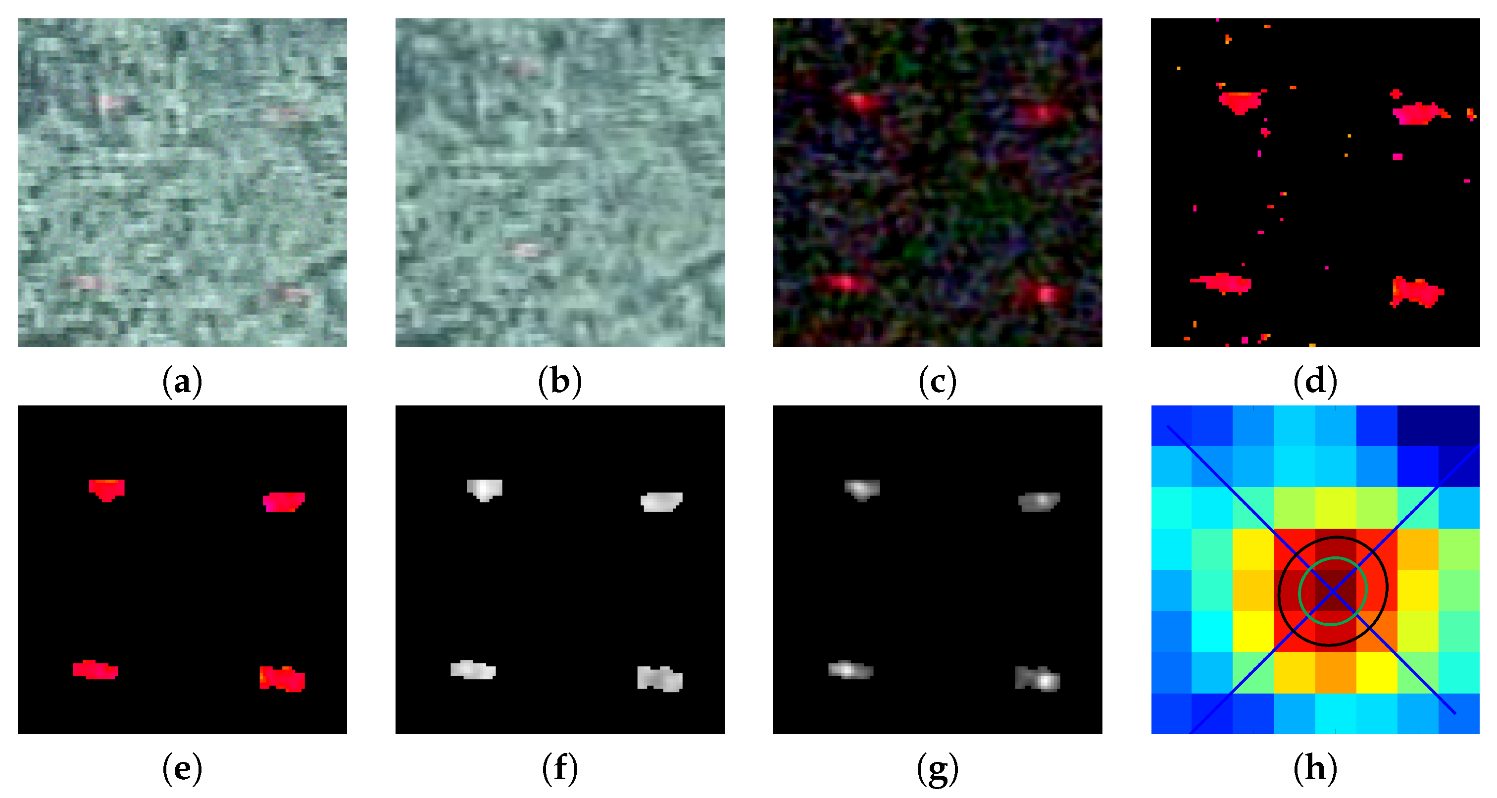
To determine laser spot positions on any image, the first step is a restriction of the search area to a patch where visible laser spots are expected (Figure 8a). Although not compulsory, this restriction minimizes false detections and reduces computational complexity and cost. The predicted area may be determined from the general pose of the lasers with respect to the camera, and from the range of distances to the scene.

An auxiliary image is used to obtain a pixel-wise aligned description of the texture in the patch. This additional image is assumed to be acquired at a similar distance and with laser spots either absent or in different positions. This ensures visually similar texture information at the positions of the laser spots. This requirement is easily achievable for video acquisitions, as minor changes in camera pose sufficiently change the positions of the lasers. Alternatively, if still images are acquired, in addition to each image with visible laser spots, an additional image taken from a slightly different pose or in the absence of laser projections has to be recorded. The appropriate auxiliary patch is determined using normalized cross correlation in Fourier domain [70] using the original patch and the auxiliary image. The patch is further refined using a homography transformation estimated by enhanced correlation coefficient maximization [71] (Figure 8b). Potential discrepancies caused by the changes in the environment between the acquisitions of the two images, are further reduced using histogram matching. Once estimated, the texture is removed from the original patch to reduce the impact of the texture on the laser beam spots. A low-pass filter further reduces noise and the effect of other artifacts (e.g., image compression), before detection using color thresholding (e.g., red color) in the HSV (Hue, Saturation, and Value) color space (Figure 8d). Pixels with low saturation values are discarded as hue cannot be reliably computed. The remaining pixels are further filtered using mathematical morphology (opening operation). The final laser spots are selected by connected-component analysis (Figure 8e).

Once the effects of the scene texture have been eliminated, the highest intensity point may be assigned to the laser beam center. In our procedure, the beam luminosity is characterized by the V channel of the HSV image representation. Figure 8f,g depicts the estimate of the laser beam luminosity with and without texture removal. Our proposed texture removal step clearly recovers the characteristic shape of the beam, with radially decreasing intensity from the center. Fitting a 2D Gaussian distribution to each laser spot allows us to estimate the center of the beam, assuming a $95\%$ probability that the center falls within the top $20\%$ of the luminance values (Figure 8h).

4.2. Uncertainty

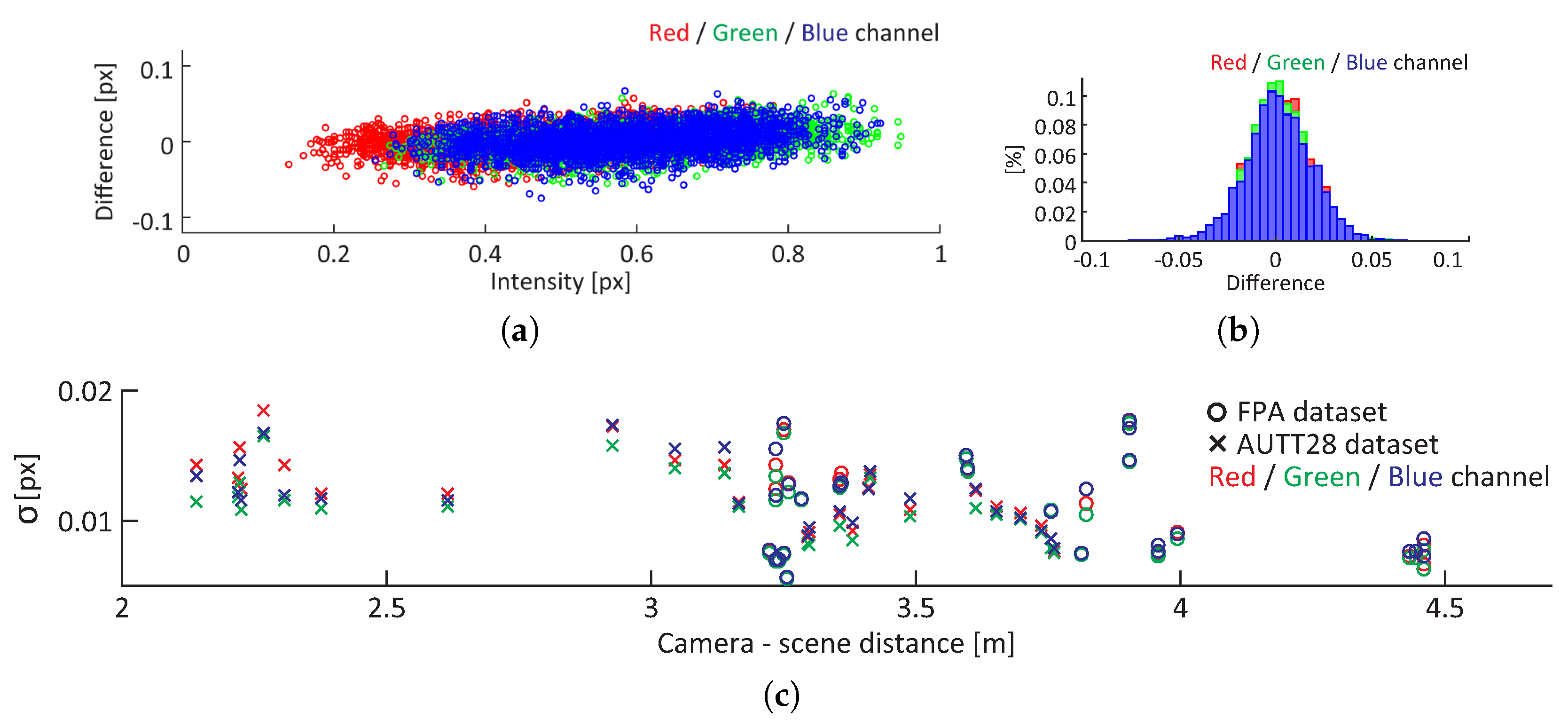
Given that the estimation of the laser center is based on color information, it is important to consider the effect of image noise. Depending on the particularities of the image set, image noise is the result of the combined effects of sensor noise, image compression, and motion blur, among others. In our approach, the image noise is characterized by comparing the same area in two images taken within a short time interval (e.g., time between two consecutive frames), where the sensed difference can be safely attributed to image noise rather than an actual change in the environment.

For a randomly selected image from dataset FPA, the relation between assumed image noise (pixel-wise difference of intensities) and pixel intensities per color channel is depicted in Figure 9a, with the histogram of differences shown in Figure 9b. The results clearly illustrate a lack of correlation between image noise and pixel intensity levels or color channels as well as the fact that the noise can be well described by a Gaussian distribution. Furthermore, the analysis of 52 images from both datasets (FPA and AUTT28), acquired at a wide range of camera–scene distances and locations, in which the image noise was approximated by Gaussian distribution, indicating that the distribution of noise remains bounded regardless of the dataset or camera–scene distance (Figure 9c). While it is worth noting that the motion blur will be increasingly noticeable in images acquired at closer ranges, the analyzed range of distances is representative of the ones used for the evaluation presented in the following sections.

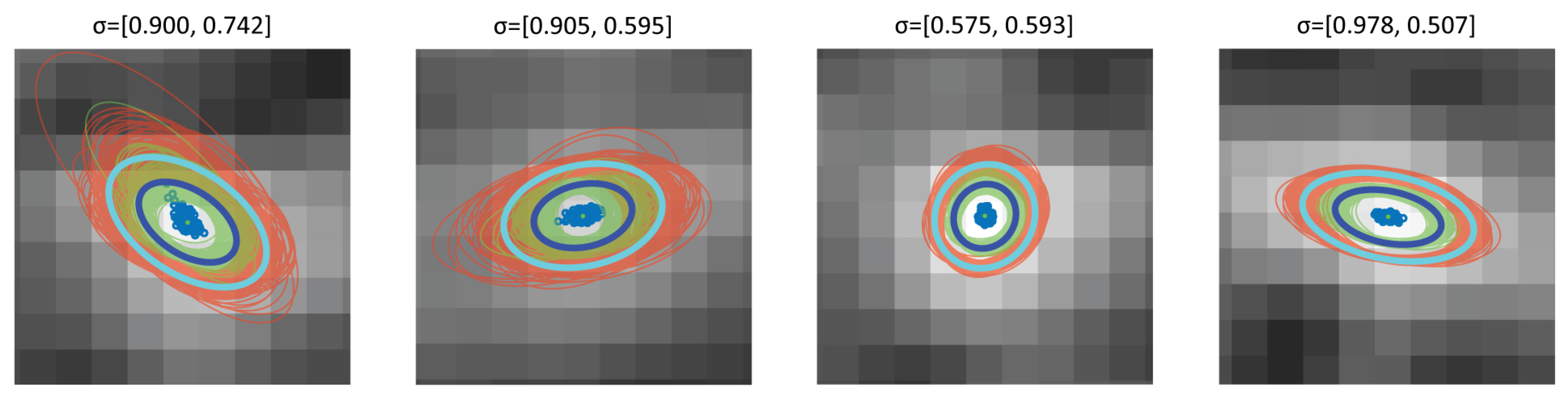
To obtain a final estimate of confidence levels of detection, the uncertainty of image intensities are propagated through the laser detection process using MC simulation. At each iteration the noise is added independently to each pixel before the described laser spots detection. The iterations yield a set of independent detections, each characterized by a Gaussian distribution (Figure 8h). The final laser spot detection is subsequently obtained by determining an equivalent Gaussian using the Unscented Transform [72] to make this process less computationally expensive. If the laser is not detected in more than $80\%$ of iterations, the detection is considered unstable and discarded. A set of laser spot detections obtained by a MC simulation is shown in Figure 10, together with the final joint estimation. Red and green ellipses represent $66\%$ and $95\%$ confidence levels for independent detections, while blue and cyan indicate the final (combined) uncertainty.

5. Dataset

During the SUBSAINTES 2017 cruise (doi: 10.17600/17001000) [43] extensive seafloor imagery was acquired with the ROV VICTOR 6000 (IFREMER) [73]. The cruise targeted tectonic and volcanic features off Les Saintes Islands (French Antilles), at the same location as that of the model published in an earlier study [9], and derived from imagery of the ODEMAR cruise (doi: 10.17600/13030070). One of the main goals of this cruise was to study geological features associated with a recent earthquake—measuring the associated displacement along a fault rupture—while expanding a preliminary study that presented a first 3D model where this kind of measurement was performed [9]. To achieve this, the imagery was acquired at more than 30 different sites along $\sim 20\mathrm{k}\mathrm{m}$, at the base of a submarine fault scarp. This is, therefore, one of the largest sets of image-derived underwater 3D models acquired with deep sea vehicles to date.

The ROV recorded HD video with a monocular camera (Sony FCB-H11 camera with corrective optics and dome port) at 30Hz, and with a resolution of $1920\times 1080$ px (Figure 11). Intrinsic camera parameters were determined using a standard calibration procedure [74] assuming a pinhole model with the 3rd degree radial distortion model. The calibration data was collected underwater using a checkerboard of $12\times 8$ squares, with identical optics and camera parameters as those later used throughout the entire acquisition process. The final root mean square (RMS) re-projection error of the calibration was (0.34 px, 0.30 px). Although small changes due to vibrations, temperature variation, etc. could occur, these changes are considered too small to significantly affect the final result.

Onboard navigation systems included a Doppler velocity log (Teledyne Marine Workhorse Navigator), fibre-optic gyrocompass (iXblue Octans), depth sensor (Paroscientific Digiquartz), and a long-range USBL acoustic positioning system (iXblue Posidonia) with a nominal accuracy of about $1\%$ of the depth. As the camera was positioned on a pan-and-tilt module lacking synchronization with the navigation data, only the ROV position can be reliably exploited.

To date, 3D models have been built at more than 30 geological outcrops throughout the SUBSAINTES study area. Models vary in length between $\sim 10\mathrm{m}$ and $\sim 300\mathrm{m}$ horizontally, and extend vertically up to $30\mathrm{m}$. Here we select two out of the 30 models (FPA and AUTT28), representative both of different survey patterns and spatial extents and complexity. Concurrently, evaluation data were collected with the same optical camera centered around a laser scaler consisting of four laser beams. For both selected datasets, numerous laser observations were collected, ensuring data spanning throughout the whole area. This enabled us to properly quantify the potential scale drifts within the models.

5.1. FPA

The first model (named FPA), extends laterally $33\mathrm{m}$ and $10\mathrm{m}$ vertically, and corresponds to a subvertical fault outcrop at a water depth of $1075\mathrm{m}$. The associated imagery was acquired in a $10\min$ $51\mathrm{s}$ video recording during a single ROV dive (VICTOR dive 654). To fully survey the outcrop, the ROV conducted multiple passes over the same area. In total, 218 images were selected and successfully processed to obtain the final model shown in Figure 12. The final RMS re-projection errors of BA using different strategies are reported in

Table 1. Final RMS re-projection error (in pixels) achieved for the reconstructions of the FPA and AUTT28 models using all four strategies.

	FPA	AUTT28
Global SfM w/Similarity T.	0.42	0.44
Incremental SfM w/Similarity T.	0.37	0.36
Global SfM w/multiobjective BA	0.49	0.74
Incremental SfM w/multiobjective BA	0.44	0.56

. As expected, the optimizations using solely visual information and incremental approach are able to achieve lower re-projection errors, which, however, is not sufficient proof of an accurate reconstruction.

5.2. AUTT28

The second model (named AUTT28), shown in Figure 13, is larger and required a more complex surveying scenario, as is often encountered in real oceanographic cruises. Initially, the planned area of interest was recorded during VICTOR dive 654. Following a preliminary onboard analysis of the data, a vertical extension of the model was required, which was subsequently surveyed during VICTOR dive 658. This second survey also partially overlapped with the prior dive, with overlapping images acquired at a closer range and thus providing higher textural detail. The survey also included a long ROV pass with the camera nearly parallel to the vertical fault outcrop, an extremely undesirable imaging setup. This second 3D model is the largest constructed in this area, covering a sub-vertical fault scarp spanning over $300\mathrm{m}$ laterally and $10\mathrm{m}$ vertically, with an additional section of approximately $30\mathrm{m}$ in height from a vertical ROV travel. This model is thus well suited to evaluate scaling errors associated with drift as it includes several complexities (survey strategy and geometry, multiple dives, extensive length and size of the outcrop). After keyframe selection, 821 images were used out of a combined $1\mathrm{h}$ $28\min$ and $19\mathrm{s}$ of video imagery to obtain reconstructions with the RMS re-projection error, as reported in Table 1.

5.2.1. Multiobjective BA Weight Selection

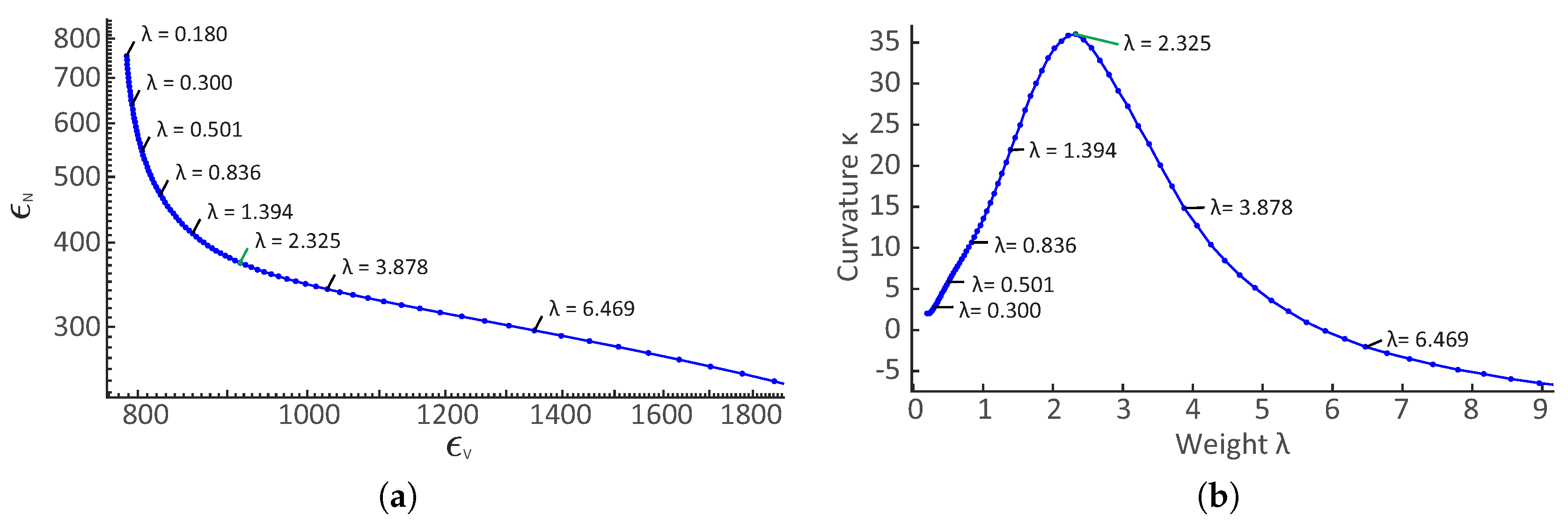
Models built with a priori navigation fusion through the multiobjective BA strategy require a weight selection which represents the ratio between re-projection and navigation fit errors. As uncertainties of the two quantities are in different units and, more importantly, not precisely known, this selection must be done either empirically or automatically. Due to the tedious and potentially ambiguous trial-and-error approach of empirical selection, the weight was determined using L-Curve analysis.

The curve, shown in Figure 14a, uses the FPA dataset and 100 BA repetitions with weights $\lambda$ ranging from $0.18$ to 18. As predicted, the shape of the curve resembles an “L”, with two dominant parts. The point of maximum curvature is determined to identify the weight with which neither objective has dominance (Figure 14b). As noise levels of the camera and navigation sensors do not significantly change between the acquisition of different datasets, the same optimal weight $\lambda =\mathbf{2.325}$ was used in all our multiobjective optimizations.

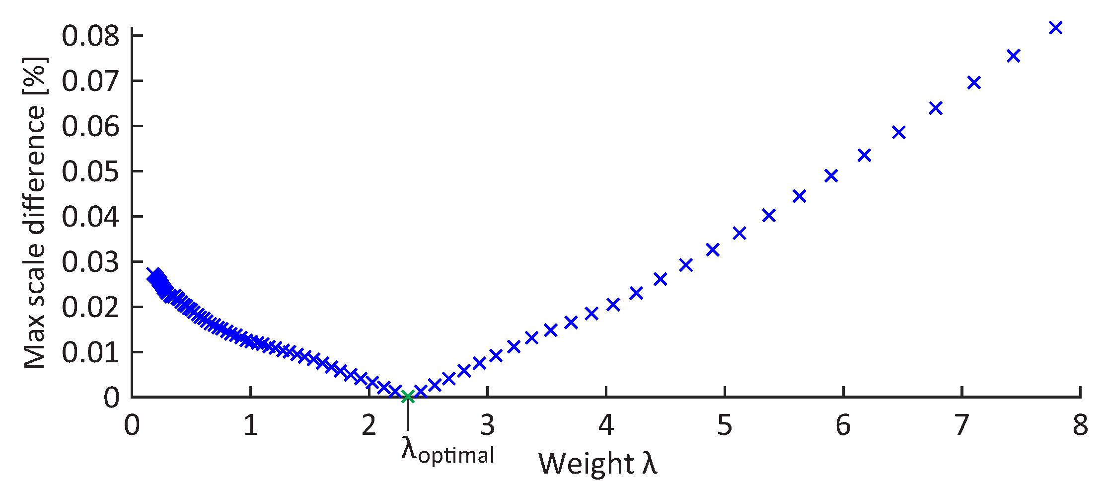
Given the heuristic nature of the optimal weight determination, it is important to evaluate the effects of the selection uncertainty on the final results. Figure 15 depicts the maximum difference in scale between the reconstructions computed using different weights and the reconstruction obtained with the optimal weight. The maximum expected scale differences were determined by comparing the Euclidean distances between the cameras of various reconstructions. The scale of the model is not expected to change if the ratio between the position of cameras does not change. The results show that the scale difference increases for an approximately $1\%$ with the increment or decrement of $\lambda$ by a value of one. Given that the optimal $\lambda$ can be determined with the uncertainty of less than $0.1$, as illustrated in Figure 14b, it can be assumed that the uncertainty in the determination of optimal weight has no significant effect on the final result.

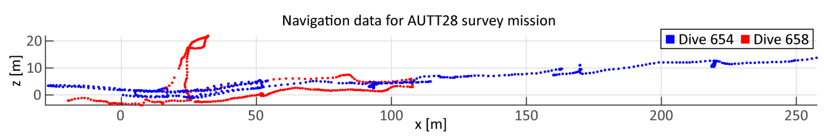
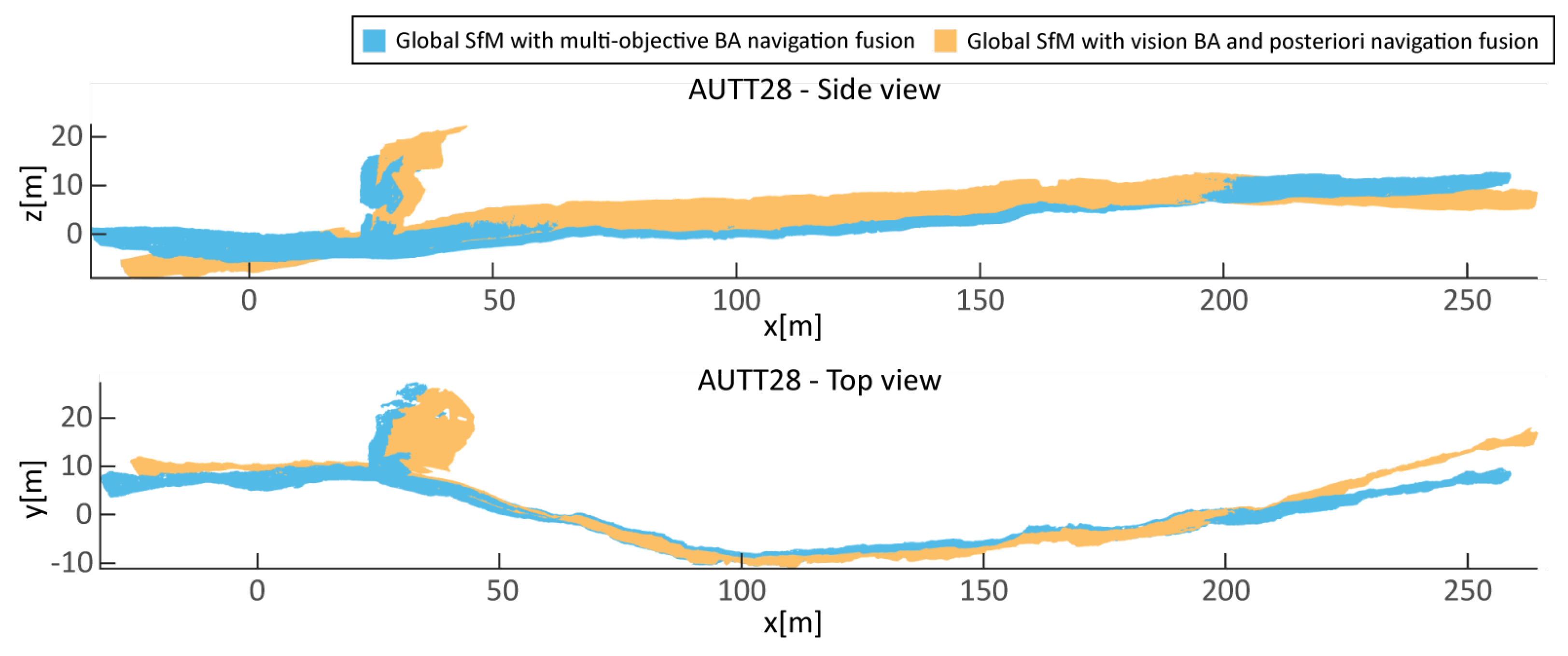
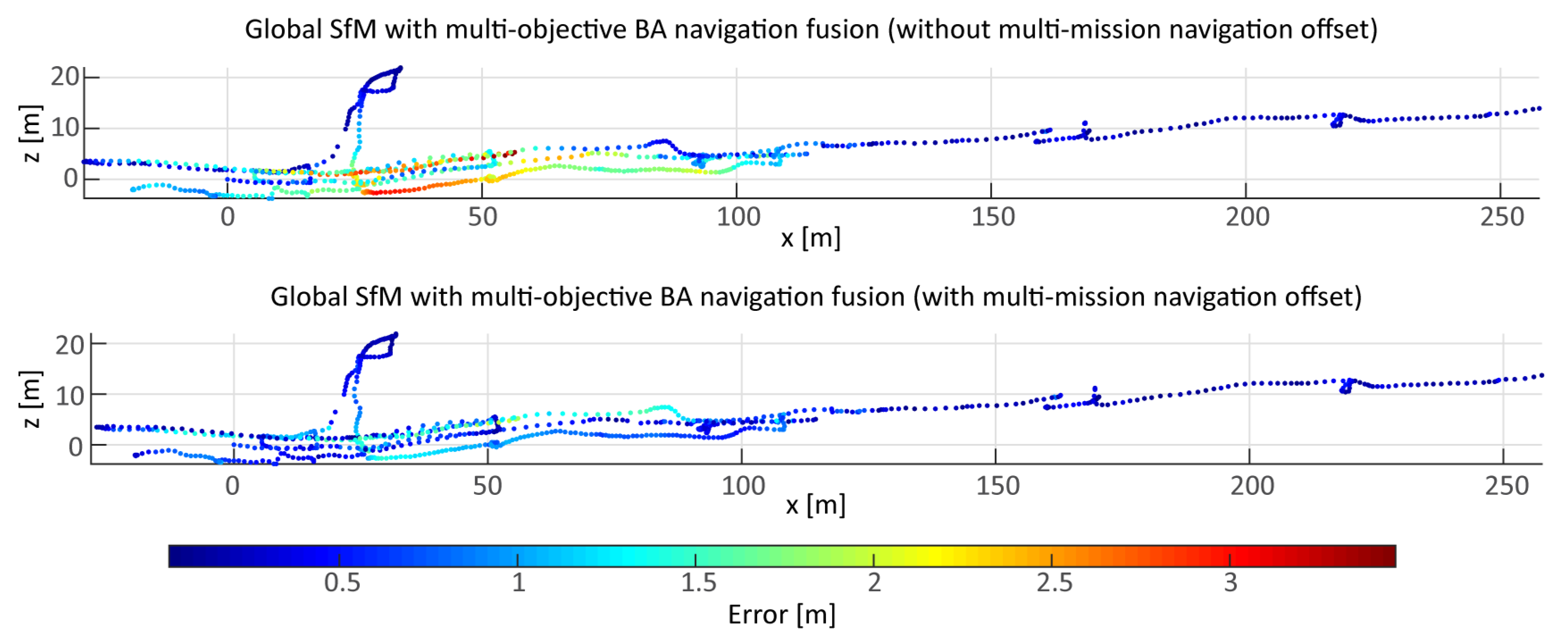
5.2.2. Multisurvey Data

As is often the case in real cruise scenarios, the data for the AUTT28 model was acquired in multiple dives (Figure 16). When combining the data, it is important to consider the consequences of the merger. Optical imagery can be simply combined, given the short period of time between the two dives, in which no significant changes are expected to occur in the scene. In contrast, the merging of navigation data may be challenging; ROV navigation is computed using smoothed USBL and pressure sensor data, with expected errors in acoustic positioning being ~$1\%$ deep. As data was collected at roughly $1000\mathrm{m}$ depth, the expected nominal errors are $\sim 10\mathrm{m}$, or more in areas of poor acoustic conditions (e.g., close to vertical scarps casting acoustic shadows or reverberating acoustic pings). These errors, however, do not represent the relative uncertainty between nearby poses, but rather a general bias of the collected data for a given dive. Although constant within each dive, the errors can differ between the dives over the same area, and are problematic when data from multiple dives are fused. Models built with data from a single dive will only be affected by a small error in georeferencing, while multisurvey optimization may have to deal with contradicting navigation priors; images taken from identical positions would have different acoustic positions, with offsets of the order of several meters or more.

This is overcome by introducing an additional parameter to be estimated, in the form of a 3D vector for each additional dive, representing the difference between USBL-induced offsets. Each vector is estimated simultaneously with the rest of the parameters in the SfM. For the case of AUTT28, the offset between the dives 654 and 658 was estimated to be $-2.53\mathrm{m}$, $1.64\mathrm{m}$, and $-0.02\mathrm{m})$ in the x (E-W), y (N-S), and z (depth) directions, respectively. The disproportionately smaller z offset is due to the fact that the pressure sensor yields inter-dive discrepancies that are orders of magnitude smaller than the USBL positions.

5.3. Laser Calibration

Normally, the calibration process consists of the initial acquisition of images containing clearly visible laser beam intersections with a surface at a range of known or easily determined distances (e.g., using a checkerboard pattern). The 3D position of intersections, expressed relative to the camera, can be subsequently computed through the exploitation of the known 2D image positions and aforementioned camera–scene distances. Given a set of such 3D positions spread over a sufficient range of distances, the direction of the laser can be computed through a line-fitting procedure. Finally, the origin is determined as the point where the laser line intersect the image plane. Given the significant refraction at the air–acrylic–water interfaces of the laser housing, the images used in the calibration process must be collected under water.

In our case, the evaluation data was collected during multiple dives separated by several days, and with camera and lasers being mounted and dismounted several times. While the laser-scaler mounting brackets ensured that the laser origins remained constant, the laser directions with respect to the camera changed slightly with each installation. Due to operational constraints on the vessel, it was not possible to collect dedicated calibration data before each dive. However, given that the origins of the lasers are known a priori and remained fixed throughout the cruise, the only unknown in our setup is the inter-dive variation of the laser directions (relative to the camera and with respect to each other). The fact that independent laser directions do not encapsulate scale information (only the change of direction on an arbitrary unit) enables us to overcome the lack of dedicated calibration images and alternatively determine the set of points lying on each laser beam using images collected over the same area for which a 3D model has been constructed.

As our interest is only in the laser directions, the points used in the calibration can be affected by an arbitrary unknown scale factor, as long as this factor is constant for all of the points. Therefore, it is important to avoid models with scale drift, or to use data from multiple models with different scales. For each of the images used in the calibration, the camera was localized with respect to the model by solving an PnP problem [65] as in the FUM and PCM and additionally refined through BA. Each of the individual laser points were then determined by a ray-cast process and expressed in the camera coordinate system, before the direction of each of the lasers was determined by line-fitting. To maximize the conditioning of line-fitting, the selection of a model with the widest distance range of such intersection points and the smallest scale drift is important. This is the case for the AUTT28 model built using Global SfM and multiobjective BA, selected here. The global nature of the SfM and internal fusion of navigation data is predicted to most efficiently reduce a potential scale drift. As noisy laser detections are used to obtain the 3D points utilized in the calibration, laser spot uncertainties were propagated to obtain the associated uncertainty of the estimated laser direction. A MC simulation with a 1000 repetitions was used. Together with the a priori known origin of the laser, this calibration provides us with all the information needed to perform scale estimation using the fully-unconstrained method.

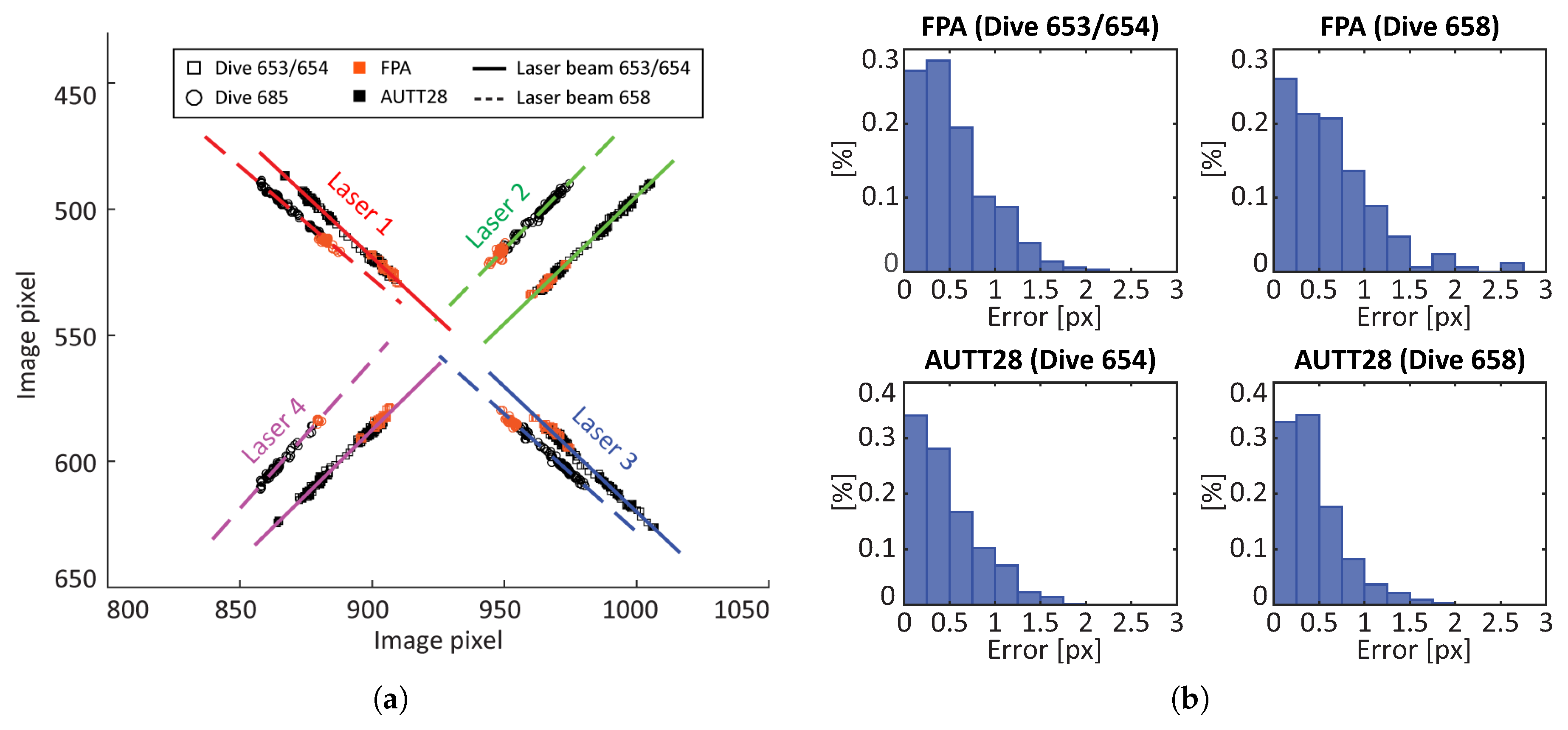
The evaluation data were collected on dives 653, 654, and 658. As no camera and laser dismounting/mounting occurred between dives 653 and 654, there are two distinct laser setups: one for dives 653 and 654 and one for dive 658. Figure 17a depicts all laser intersections with the scene (for both AUTT28 and FPA models), as well as the calibration results, projected onto an image plane. Intersections detected in 3D model AUTT28 are depicted in black, and those from 3D model FPA are shown in orange. Similarly, the squares and circles represent dives 653/654 and dive 658, respectively. The projections of the final laser beam estimations are presented as solid and dotted lines. The figure shows a good fit of estimated laser beams with the projections of the intersections, both in the AUTT28 and FPA models.

The distributions of calibration errors, measured as perpendicular distances between the calibrated laser beams and the projected laser intersections with the scene, are depicted in Figure 17b, and the RMS errors are listed in

Table 2. RMS calibration errors (in pixels) measured as perpendicular distances between the projected laser beams and laser intersections with the scene for the two datasets and dives.

Dataset	FPA		AUTT28
Dive	653/654	658	654	658
RMSE [px]	0.66	0.79	0.60	0.55

. The adequate fit to the vast majority of AUTT28 points (RMS error < $0.6$px) shows that the model used in the calibration had no significant scale drift. Furthermore, the fitting of the FPA related points (RMS error < $0.8$px), which were not used in the calibration and are affected by a different scale factor, confirms that the calibration of laser directions is independent of the 3D model used, as well as of different scalings. The broad spread of the black points relative to the orange ones also confirms that the choice of the AUTT28 over the FPA model was adequate for this analysis. Lastly, it is worth reiterating that the data from all the models cannot be combined for calibration, as they are affected by different scale factors.

6. Results

As the accuracy of the measurements performed in 3D models for the purposes of quantitative studies (precise measurement of distances and volumes, etc.) depends on the strategy used for image-based 3D reconstruction, in addition to data quality itself, four of the most widely used approaches were evaluated:

A) 

Incremental SfM with a posteriori navigation fusion.

B) 

Global SfM with a posteriori navigation fusion.

C) 

Incremental SfM with multiobjective BA navigation fusion.

D) 

Global SfM with multiobjective BA navigation fusion.

The models for each of the two datasets (FPA and AUTT28) were built using each of the four strategies, and subsequently evaluated on multiple segments spread across the observed area. Using the model evaluation framework and laser spot detection method presented above, the scale accuracy and its associated uncertainties were automatically estimated using more than 550 images. To minimize the effects of possible false laser spot detections, only images with at least two confidently detected laser points were used. Furthermore, any images exhibiting excessive variation of the estimated scale between the individual lasers were discarded, as scale can be assumed to be locally constant.

6.1. Scale Accuracy Estimation

During accuracy evaluation, the scale error ${ϵ}_s$ is estimated for each image independently. The final per-image scale error and its uncertainty are estimated through a MC simulation, with input variables (features, laser spot locations and laser calibration) sampled according to their probability distributions. The repeated computation with noisy data thus results in an equal number of final scale error estimates per laser. Figure 18 shows one example of such an estimation, together with the selected intermediate results of the evaluation process. As each MC iteration encapsulates the complete evaluation process (image localization, ray-casting, origin estimation, and scale error evaluation), intermediate distributions presented in Figure 18 are only shown for illustration, and are not used as distribution assumptions in the process itself.

To satisfactorily represent the complexity of the process, 5000 iterations were used for each estimation. Figure 19 shows the evolution of the estimated scale error with associated uncertainty with increasing number of samples. After 500 iterations, the errors exhibit only minor fluctuations, and after 1500 iterations there is no noticeable difference. Hence, our selection of 5000 iterations is more than adequate to encapsulate the distribution of noise.

To demonstrate the advantages of our fully-unconstrained approach compared to previously available methods or our partially-constrained method, scale estimates obtained for each laser/laser pair are compared. Given the nonalignment of lasers with the optical axis of the camera, the majority of previous image-scaling methods (e.g., [24,25]) are not applicable. The only available option is thus a simplified approach where the Euclidean distance between a pair of 3D points (laser intersection points with the scene) is assumed to be the actual distance between the laser pair.

Results using different lasers (Figure 20) show that the FUM method produces the most consistent results. This is expected as the estimation process considers both individual laser directions and the geometry of the scene. The effect of scene geometry is clear when Figure 20a,b are compared. The slightly slanted angle together with the uneven geometry of the scene causes a large variation in the scale error estimates by the individual laser pairs. Similarly, the comparison of Figure 20b,c shows the effect of an inaccurate assumption of laser parallelism. This error depends on the camera–scene distance as shown in Figure 21. It is likely that the overestimation of laser pair 3–4 and the underestimation of other laser pairs can be explained by the use of oversimplified laser geometry. To validate this assumption, the results of the partially-constrained method were corrected by the expected errors (at $d=2m$) induced by disregarding nonparallelism of laser beams (Figure 20d). While the result is nearly identical to that from a FUM method (Figure 20c), we note that the scale error in Figure 20c is computed for each laser individually, while the partially-constrained method considers laser pairs instead, and hence there are minor discrepancies.

6.2. FPA

The accuracy of the FPA model was analyzed using 148 images (432 lasers). To represent the results concisely, measurements are grouped into 7 segments based on their model position (Figure 22 and

Table 3. Distribution of laser observations per segment for FPA area.

	A	B	C	D	E	F	G
# Images	12	6	39	40	12	24	15
# Lasers	29	12	137	103	33	53	36
Laser distance (min/max) [$\mathrm{m}$]	3.23/3.29	4.44/4.46	3.03/3.50	3.58/4.01	3.59/3.61	3.19/3.37	3.19/3.79

). To ensure that the scale of the model did not vary within each segment, the maximum distance of any laser detection to the assigned segment center was set to $1\mathrm{m}$.

FPA covers a relatively small area, and is imaged with multiple passes, thus providing redundancy that promotes model accuracy. Hence, it is expected to have only minor variations in scale error between areas. Figure 23 depicts the distribution of estimated scale errors for all four methods of 3D model construction. The comparison of results (

Table 4. Estimated scale errors (%) per segment for different reconstructions of FPA area (values represent mean value with standard deviation).

	A	B	C	D	E	F	G
Global SfM w/Similarity T.	$-3.6\pm 2.9$	$0.9\pm 3.2$	$-1.1\pm 1.9$	$-1.2\pm 3.4$	$-1.4\pm 2.8$	$-4.0\pm 2.9$	$-4.0\pm 3.4$
Incremental SfM w/Similarity T.	$-3.6\pm 2.9$	$0.9\pm 3.2$	$-1.0\pm 1.9$	$-1.2\pm 3.4$	$-1.4\pm 2.8$	$-4.0\pm 2.9$	$-4.0\pm 3.5$
Global SfM w/multiobjective BA	$-4.7\pm 2.8$	$0.7\pm 3.2$	$-1.3\pm 1.9$	$-1.2\pm 3.4$	$-1.4\pm 2.8$	$-3.1\pm 2.9$	$-2.2\pm 3.5$
Incremental SfM w/multiobjective BA	$-4.7\pm 2.9$	$0.7\pm 3.2$	$-1.3\pm 1.9$	$-1.2\pm 3.4$	$-1.4\pm 2.8$	$-3.2\pm 2.9$	$-2.1\pm 3.5$

) shows that accuracy does not significantly differ between them. The scale error varies between $-1\%$ and $-5\%$ with estimated uncertainties of approximately $\pm 3\%$. The highest errors occur at the borders of the model. As expected, uncertainty is closely related to the camera–scene distance, as small uncertainties in the laser direction translate to larger discrepancies at larger distances.

6.3. AUTT28

For model AUTT28, the evaluation data (images containing projected laser spots) were gathered during VICTOR dives 654 and 658, after the video acquisition of data used for 3D model creation. A total of 432 images with 1378 laser measurements were selected and grouped into 6 distinct sections throughout the 3D model, as shown in

Table 5. Distribution of laser observations per segment for AUTT28 area.

	A	B	C	D	E	F
# Images	30	47	20	46	261	28
# Lasers	97	169	51	165	812	84
Laser distance (min/max) [$\mathrm{m}$]	1.95/2.25	2.13/2.67	2.90/3.36	3.21/3.89	1.70/4.14	3.63/3.79

and Figure 24. Dive 654 covered a longer vertical path (blue dots), while dive 658 (red dots) surveyed an additional horizontal segment together with parts of the area already viewed using dive 654. The higher density of red points indicates that the ROV observed the scene at a closer range during dive 658, requiring a higher number of images to obtain the necessary overlap compared to dive 654.

The comparison of results (

Table 6. Estimated scale errors (%) per segment for different reconstructions of AUTT28 area (values represent mean value with standard deviation).

	A	B	C	D	E	F
Global SfM w/ Similarity T.	$-6.4\pm 2.3$	$-6.3\pm 1.9$	$-4.5\pm 2.4$	$-1.1\pm 2.0$	$2.1\pm 2.2$	$9.2\pm 2.9$
Incremental SfM w/Similarity T.	$-6.3\pm 2.3$	$-6.1\pm 1.9$	$-4.1\pm 2.5$	$-0.8\pm 2.0$	$2.3\pm 2.3$	$9.3\pm 2.8$
Global SfM w/multiobjective BA	$0.7\pm 2.4$	$0.7\pm 2.0$	$0.8\pm 2.6$	$-0.2\pm 2.0$	$1.7\pm 2.3$	$0.9\pm 2.6$
Incremental SfM w/multiobjective BA	$-0.6\pm 2.4$	$-0.1\pm 2.1$	$1.2\pm 2.6$	$2.0\pm 2.2$	$1.7\pm 2.3$	$0.6\pm 2.7$

) shows that the models built using a posteriori navigation fusion (Figure 25a,b) are significantly impacted by scale drift ($\sim 15\%$), and that this impact is nearly identical regardless of the use of global or incremental SfM approaches. The gradual scale sliding observed is caused by inherent scale ambiguity of the two-view image pair geometry when BA is solely dependent on visual information. While this might not have been as obvious in the previous case, the long single pass of the camera, as performed in dive 654, introduces in this particular model numerous consecutive two-view image pairs, magnifying the scale drift. As shown in Figure 25c,d, additional constraints in the BA (e.g., navigation data) reduce ambiguity and, ultimately, nearly eliminate scale drift. Overall, scale error of the model built with global SfM using multiobjective BA is less than $1\%$ with nearly zero scale drift, while a model built with incremental SfM approach showed a $2\%$ scale drift along its $300\mathrm{m}$ length. It should be noted that the observed difference in scale estimates are within the uncertainty levels of the estimations, and therefore inconclusive.

6.3.1. Multiobjective BA vs. Similarity Transformation Navigation Fusion

The effects of different navigation fusion strategies are further demonstrated through the comparison of two reconstructions obtained using Global SfM with multiobjective BA and with similarity transformation (Figure 26). The reconstructions diverge on the outer parts of the model, consistent with a “doming” effect. A broad-scale systematic deformation produces a reconstruction that appears as a rounded-vault-distortion of a flat surface. This effect is a result of applying a rigorous re-projection error minimization to a loosely interconnected longer sequence of images taken from a nearly parallel direction, combined with slight inaccuracies in modeling of the radial distortion of the camera [14]. Multiobjective BA is able to reduce the effect by introducing the additional non-vision-related constraints, while the similarity transformation, with its preservation of angles between any three points and subsequent shape preservation, is not adequate for such corrections of the model deformations.

6.3.2. Multisurvey Data Fusion

As explained in Section 5.2.2, the multimission data fusion can cause contradictory navigation priors during optimization. We address this by expanding the optimization problem with an additional 3D vector, representing the possible USBL offset between the recorded navigation data of the two dives. To examine the effects of this offset compensation on model construction, an additional model was constructed using raw navigation data (i.e., without offset compensation). Figure 27 depicts errors in the camera pose estimates with respect to their navigation priors, and shows a concentration of errors in areas imaged during both dives (Figure 16), where navigation priors of the two dives are incoherent. The errors dramatically decrease with the introduction of an offset, yielding an improved fitting solution. Alternatively, incoherence can cause model distortions to compensate for contradicting priors, as shown by abrupt changes of scale (area D in Figure 28).

6.3.3. Scale Error Estimation Methods

To recover high-resolution and precise information from 3D models (lengths, areas, and volumes) it is important to use the most accurate method. As the nonalignment of lasers with the optical axis of the camera prevents the use of previous image-scaling methods (e.g., Pilgrim et al. [24]; Davis and Tusting [25]), two other methods could be used instead. Minor misalignments of laser scalers may be discarded for simplicity or lack of sufficiently distributed calibration data. In such cases, both our partially-constrained approach and the simplified direct 3D method, that assumes an equivalence of the Euclidean distance between the points of laser intersections and the beams themselves, could be used for the evaluation.

For this comparison the model with least scale drift was selected (Global SfM and multiobjective BA navigation fusion) to emphasize the effects of different methods on the results. Furthermore, as both the simplistic direct 3D and partially-constrained methods assume laser-pair parallelism, the analysis of these two methods was performed on data consisting of only laser pairs that were the closest to being parallel (Figure 29a and Figure 30a), as well as on the complete dataset (Figure 29b and Figure 30b), to show the effect that nonparallelism of laser beams may have on the different methods.

As expected, in comparison to the simplistic approach (orange) (Figure 29a), our method (green) is significantly less impacted by the discrepancies in camera–scene distances at the two laser intersections caused by the deviation of camera–scene angle from perpendicularity. The spread of the estimated values within each segment for the direct approach is directly correlated with the span of camera–scene distances (most notable in area E in Figure 29). Although varying distances themselves do not play a role, they do however increase the probability of both having deviating camera-surface angles, and of violating the surface flatness requirement, which both result in discrepancies in camera–scene distances between the two laser points.

In contrast, the analysis of the results of the partially-constrained approach (Figure 30a) confirms that this method is unaffected by changes of camera angle and scene roughness. As expected, the results in sections D, E and F are nearly identical, with discrepancies in sections A, B and C. Sections A, B, and C were evaluated using data collected during dive 658, and D, E, and F were evaluated during dive 654; we attribute this discrepancy to the marginally larger error in nonparallelism of the laser configuration used during dive 658 compared to that of dive 654. This is clearly shown when the results are computed on the data from all laser pairs (Figure 30b), as nonparallelism of different laser pairs causes significant variation in the results. Segments acquired at closer ranges (A, B, and C), and therefore less affected by the errors in parallelism, have smaller errors than those of segments D and F, which are evaluated at larger distances. While similar multimodal distributions appear in the results of the simple direct 3D method, the clear multimodal peaks are suppressed by the effects of camera-surface angles and roughness of the surface model.

7. Discussion

The comparison between the results show that the fully-unconstrained method is more consistent and accurate than the two other approaches, i.e., partially-constrained and simplistic direct 3D method. We note that by limiting the data to parallel laser pairs (dive 654), the partially-constrained method produced similar results. Therefore, the PCM approach can be used when the relation between parallel lasers and the camera is not known, opening up its use to numerous scenarios where strict rigidity between the camera and lasers is not maintained or determined (e.g., legacy data).

The effects of different reconstruction strategies were analyzed using two distinct survey scenarios. The first model (FPA dataset) was acquired with multiple passes over the same areas. Overlap of nonsequential images restricted the potential solutions of the optimization problem to a nearly identical solution regardless of the strategy (SfM or navigation fusion). In a second model (AUTT28 dataset), data were acquired during two separate surveys, and include a long single pass with the camera oriented nearly parallel to a vertical wall. The results demonstrate that surveys where sequential images are weakly connected are prone to produce broad-scale deformation (doming effect) in the final model. Rigorous minimization of the re-projection error, combined with the projective scale ambiguity, distorts the model, and can lead to further drift in the scale estimate. While the navigation fusion strategy did not play a role in the first model (FPA), the results of this second model (AUTT28) demonstrate the advantage of using multiobjective BA navigation fusion to process data with more complex survey patterns. Furthermore, the introduction of additional vectors in the optimization of multisurvey problems successfully accounted for the offset changes present in the underwater USBL-based navigation data, and thus minimize the effect of contradicting navigation priors.

8. Conclusions

This study presented a comprehensive scale error evaluation of four of the most commonly used image-based 3D reconstruction strategies of underwater scenes. This evaluation seeks to determine the advantages and limitations of the different methods, and to provide a quantitative estimate of model scaling, which is required for obtaining precise measurements for quantitative studies (such as distances, areas, volumes and others). The analysis was performed on two data sets acquired during a scientific cruise (SUBSAINTES 2017) with a scientific ROV (VICTOR6000), and therefore under realistic deep sea fieldwork conditions. For models built using multiobjective BA navigation fusion strategy, an L-Curve analysis was performed to determine the optimal weight between competing objectives of the optimization. Furthermore, the potential offset in navigation when using USBL-based positioning from different dives was addressed in a representative experiment.

Building upon our previous work, the lack of readily available measurements of objects of known sizes in large scale models was overcome with the fully-unconstrained method, which exploits laser scaler projections onto the scene. The confidence level for each of the scale error estimates was independently assessed with a propagation of the uncertainties associated with image features and laser spot detections using a Monte Carlo simulation. The number of iterations used in the simulation to satisfactorily represent the complexity of the process was validated through the analysis of the final estimate behavior.

As each scale error estimate characterizes an error at a specific area of the model, independent evaluations across the models enable efficient determination of potential scale drifts. To obtain a sufficient number of accurate laser measurements, an automatic laser spot detector was also developed. By mitigating the effects of scene texture using an auxiliary image, a much larger number of accurate detections was possible, even with greatly attenuated laser beams. The requirement of having laser spots either not present or in at different position in the auxiliary image is easily satisfied in video acquisitions, while an additional image has to be recorded if still images are collected. Furthermore, the recovery of characteristic shapes of laser spots with radially decreasing intensities enabled additional determination of the uncertainty of laser spot detections. In total, the scale errors have been evaluated on a large set of measurements in both models (432/1378) spread across them.

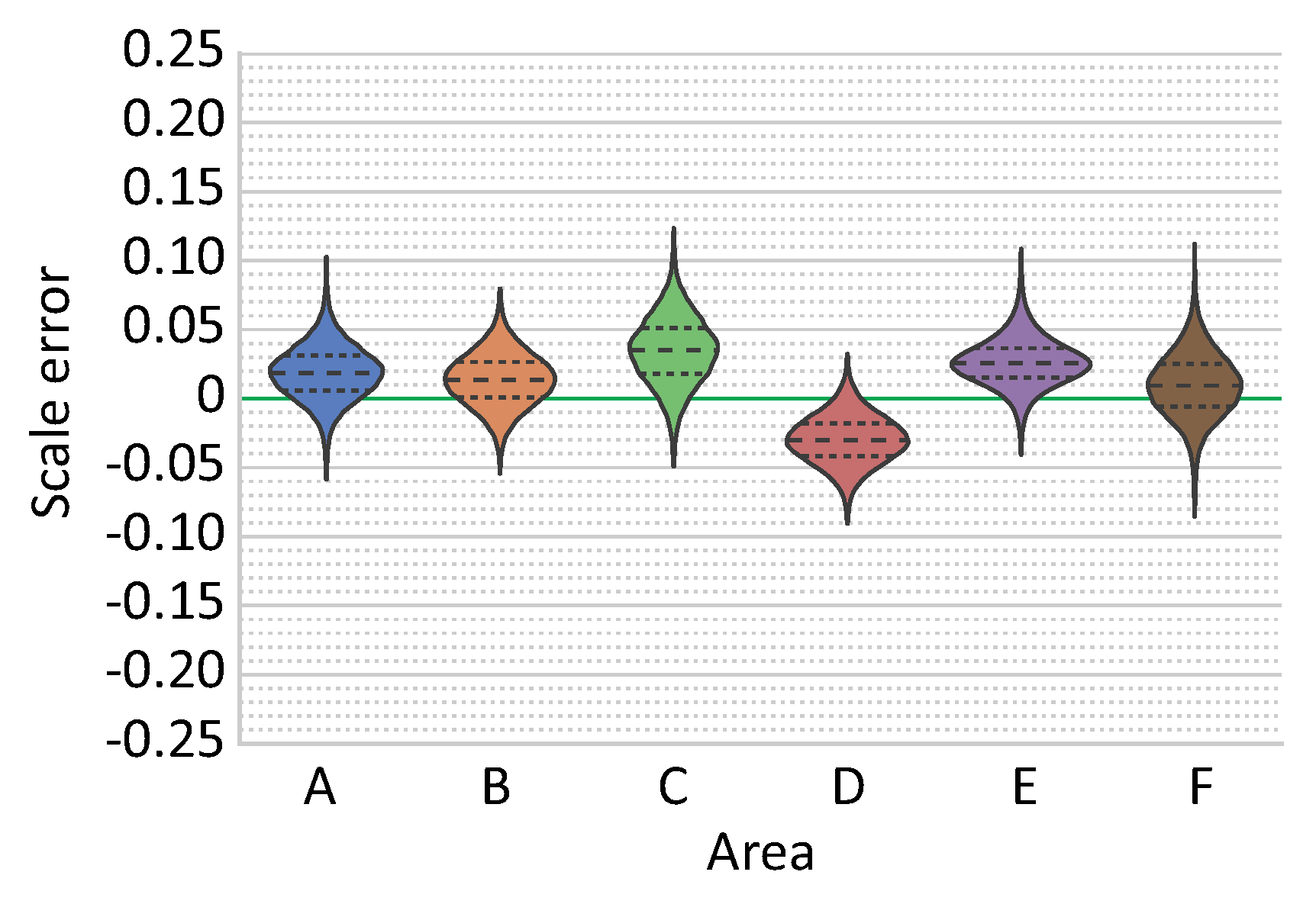
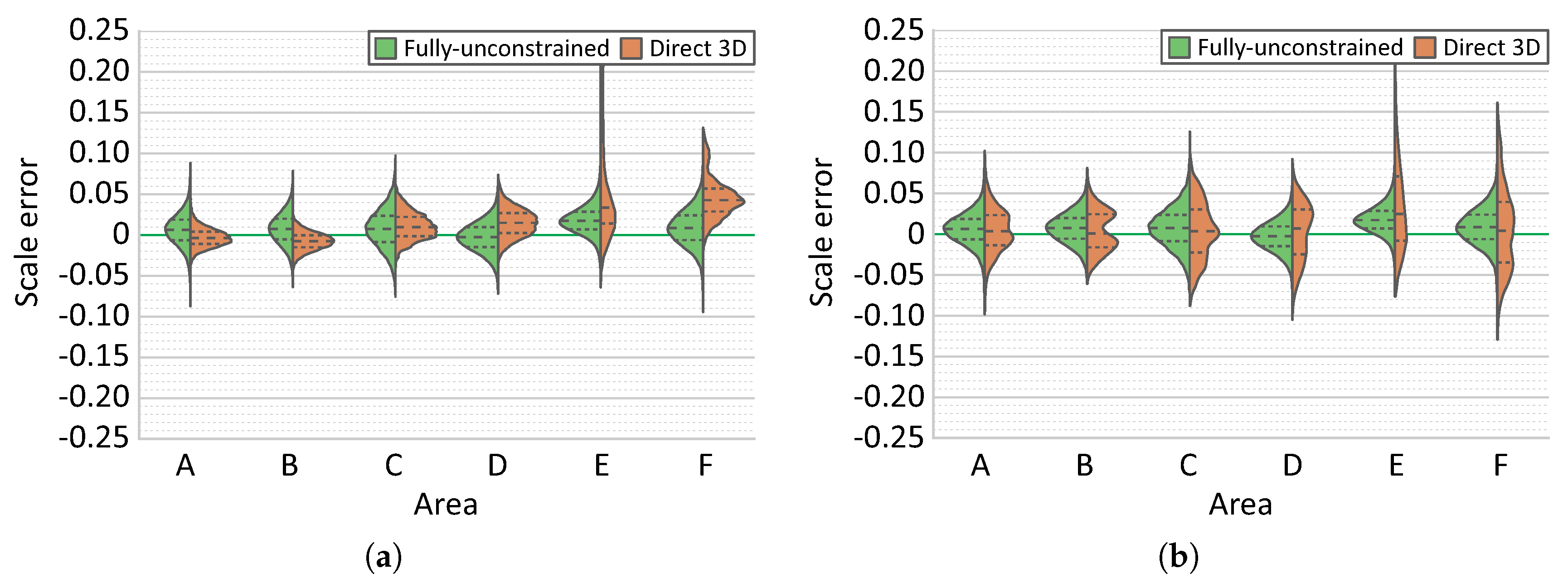
Finally, the comparison of results obtained using different reconstruction strategies were performed using two distinct survey scenarios. In surveys comprising a single dive and with multiple overlapping regions, the choice of reconstruction strategies is not critical, since all strategies perform adequately well. However, in more complex scenarios there is a significant benefit from using optimization including the navigation data. In all cases, the best reconstruction strategies produced models with scale errors inferior to $5\%$, with errors on the majority of each model area being around $1\%$. Acquisition of calibration data (points collected over a large range of distances) is indeed critical. Depending on laser setup, a modification of laser geometry is possible (e.g., during the process of diving due to pressure changes). As minor discrepancies in parallelism can cause significant offsets at the evaluating distance, performing a calibration in the field is desirable (e.g., approach of the scene illuminated with laser beams). Furthermore, our results also indicate and justify the importance of collecting a multitude of evaluation data at different locations and moments during the survey.

References

1. Lucieer, A.; de Jong, S.M.; Turner, D. Mapping landslide displacements using Structure from Motion (SfM) and image correlation of multi-temporal UAV photography. Prog. Phys. Geogr. Earth Environ. 2014, 38, 97–116. [Google Scholar] [CrossRef]
2. Javernick, L.; Brasington, J.; Caruso, B. Modeling the topography of shallow braided rivers using Structure-from-Motion photogrammetry. Geomorphology 2014, 213, 166–182. [Google Scholar] [CrossRef]
3. Marteau, B.; Vericat, D.; Gibbins, C.; Batalla, R.J.; Green, D.R. Application of Structure-from-Motion photogrammetry to river restoration. Earth Surf. Process. Landf. 2017, 42, 503–515. [Google Scholar] [CrossRef]
4. Mathews, A.J.; Jensen, J.L.R. Visualizing and Quantifying Vineyard Canopy LAI Using an Unmanned Aerial Vehicle (UAV) Collected High Density Structure from Motion Point Cloud. Remote Sens. 2013, 5, 2164–2183. [Google Scholar] [CrossRef] [Green Version]
5. Campos, R.; Garcia, R.; Alliez, P.; Yvinec, M. A surface reconstruction method for in-detail underwater 3D optical mapping. Int. J. Robot. Res. 2014, 64–89. [Google Scholar] [CrossRef]
6. Pizarro, O.; Friedman, A.; Bryson, M.; Williams, S.B.; Madin, J. A simple, fast, and repeatable survey method for underwater visual 3D benthic mapping and monitoring. Ecol. Evol. 2017, 7, 1770–1782. [Google Scholar] [CrossRef] [PubMed]
7. Bingham, B.; Foley, B.; Singh, H.; Camilli, R.; Delaporta, K.; Eustice, R.; Mallios, A.; Mindell, D.; Roman, C.; Sakellariou, D. Robotic tools for deep water archaeology: Surveying an ancient shipwreck with an autonomous underwater vehicle. J. Field Robot. 2010, 27, 702–717. [Google Scholar] [CrossRef] [Green Version]
8. Rossi, P.; Castagnetti, C.; Capra, A.; Brooks, A.; Mancini, F. Detecting change in coral reef 3D structure using underwater photogrammetry: Critical issues and performance metrics. Appl. Geomat. 2019, 1–15. [Google Scholar] [CrossRef]
9. Escartín, J.; Leclerc, F.; Olive, J.A.; Mevel, C.; Cannat, M.; Petersen, S.; Augustin, N.; Feuillet, N.; Deplus, C.; Bezos, A.; et al. First direct observation of coseismic slip and seafloor rupture along a submarine normal fault and implications for fault slip history. Earth Planet. Sci. Lett. 2016, 450, 96–107. [Google Scholar] [CrossRef]
10. Hartley, R.; Zisserman, A. Multiple View Geometry in Computer Vision, 2nd ed.; Cambridge University Press: New York, NY, USA, 2003. [Google Scholar] [CrossRef]
11. Soloviev, A.; Venable, D. Integration of GPS and vision measurements for navigation in GPS challenged environments. In Proceedings of the IEEE/ION Position, Location and Navigation Symposium, Indian Wells, CA, USA, 4–6 May 2010; pp. 826–833. [Google Scholar] [CrossRef]
12. Mian, O.; Lutes, J.; Lipa, G.; Hutton, J.; Gavelle, E.; Borghini, S. Accuracy assessment of direct georeferencing for photogrammetric applications on small unmanned aerial platforms. Int. Arch. Photogramm. Remote Sens. Spat. Inf. Sci. 2016, 40, 77. [Google Scholar] [CrossRef]
13. Forlani, G.; Dall’Asta, E.; Diotri, F.; Cella, U.M.d.; Roncella, R.; Santise, M. Quality Assessment of DSMs Produced from UAV Flights Georeferenced with On-Board RTK Positioning. Remote Sens. 2018, 10, 311. [Google Scholar] [CrossRef]
14. James, M.R.; Robson, S. Mitigating systematic error in topographic models derived from UAV and ground-based image networks. Earth Surf. Process. Landf. 2014, 39, 1413–1420. [Google Scholar] [CrossRef] [Green Version]
15. Eltner, A.; Schneider, D. Analysis of Different Methods for 3D Reconstruction of Natural Surfaces from Parallel-Axes UAV Images. Photogramm. Rec. 2015, 30, 279–299. [Google Scholar] [CrossRef]
16. Mertes, J.; Zant, C.; Gulley, J.; Thomsen, T. Rapid, quantitative assessment of submerged cultural resource degradation using repeat video surveys and Structure from Motion. J. Marit. Archaeol. 2017, 12, 91–107. [Google Scholar] [CrossRef]
17. Sedlazeck, A.; Koser, K.; Koch, R. 3D reconstruction based on underwater video from ROV Kiel 6000 considering underwater imaging conditions. In Proceedings of the OCEANS 2009-EUROPE, Bremen, Germany, 11–14 May 2009; pp. 1–10. [Google Scholar] [CrossRef]
18. Pizarro, O.; Eustice, R.M.; Singh, H. Large Area 3-D Reconstructions From Underwater Optical Surveys. IEEE J. Ocean. Eng. 2009, 34, 150–169. [Google Scholar] [CrossRef] [Green Version]
19. Campos, R.; Gracias, N.; Ridao, P. Underwater Multi-Vehicle Trajectory Alignment and Mapping Using Acoustic and Optical Constraints. Sensors 2016, 16, 387. [Google Scholar] [CrossRef] [PubMed]
20. Garcia, R.; Campos, R.; Escartín, J. High-resolution 3D reconstruction of the seafloor for environmental monitoring and modeling. In Proceedings of the 2011 IEEE/RSJ International Conference on Intelligent Robots and Systems: (IROS 2011), San Francisco, CA, USA, 25–30 September 2011. [Google Scholar]
21. Cocito, S.; Sgorbini, S.; Peirano, A.; Valle, M. 3-D reconstruction of biological objects using underwater video technique and image processing. J. Exp. Mar. Biol. Ecol. 2003, 297, 57–70. [Google Scholar] [CrossRef]
22. Kalacska, M.; Lucanus, O.; Sousa, L.; Vieira, T.; Arroyo-Mora, J. Freshwater fish habitat complexity mapping using above and underwater structure-from-motion photogrammetry. Remote Sens. 2018, 10, 1912. [Google Scholar] [CrossRef]
23. Neyer, F.; Nocerino, E.; Gruen, A. Monitoring coral growth - The dichotomy between underwater photogrammetry and geodetic control network. Int. Arch. Photogramm. Remote Sens. Spat. Inf. Sci. 2018, 42, 2. [Google Scholar] [CrossRef]
24. Pilgrim, D.A.; Parry, D.M.; Jones, M.B.; Kendall, M.A. ROV Image Scaling with Laser Spot Patterns. Underw. Technol. 2000, 24, 93–103. [Google Scholar] [CrossRef]
25. Davis, D.; Tusting, R. Quantitative Benthic Photography Using Laser Calibrations; Undersea World: San Diego, CA, USA, 1991. [Google Scholar]
26. Istenič, K.; Gracias, N.; Arnaubec, A.; Escartin, J.; Garcia, R. Automatic Scale Estimation of Structure from Motion based 3D Models using Laser Scalers. arXiv 2019, arXiv:1906.08019. [Google Scholar]
27. Nornes, S.M.; Ludvigsen, M.; Ødegard, Ø.; SØrensen, A.J. Underwater Photogrammetric Mapping of an Intact Standing Steel Wreck with ROV. IFAC-PapersOnLine 2015, 48, 206–211. [Google Scholar] [CrossRef]
28. Warren, M.; Corke, P.; Pizarro, O.; Williams, S.; Upcroft, B. Visual sea-floor mapping from low overlap imagery using bi-objective bundle adjustment and constrained motion. In Proceedings of the Australasian Conference on Robotics and Automation, Wellington, New Zealand, 3–5 December 2012. [Google Scholar]
29. Strasdat, H.; Montiel, J.; Davison, A.J. Scale drift-aware large scale monocular SLAM. Robot. Sci. Syst. VI 2010, 2, 7. [Google Scholar] [CrossRef]
30. Fonstad, M.A.; Dietrich, J.T.; Courville, B.C.; Jensen, J.L.; Carbonneau, P.E. Topographic structure from motion: A new development in photogrammetric measurement. Earth Surf. Process. Landf. 2013, 38, 421–430. [Google Scholar] [CrossRef]
31. Thoeni, K.; Giacomini, A.; Murtagh, R.; Kniest, E. A comparison of multi-view 3D reconstruction of a rock wall using several cameras and a laser scanner. Int. Arch. Photogramm. Remote Sens. Spat. Inf. Sci. 2014, 40, 573. [Google Scholar] [CrossRef]
32. Kalacska, M.; Chmura, G.; Lucanus, O.; Berube, D.; Arroyo-Mora, J. Structure from motion will revolutionize analyses of tidal wetland landscapes. Remote Sens. Environ. 2017, 199, 14–24. [Google Scholar] [CrossRef]
33. Bythell, J.; Pan, P.; Lee, J. Three-dimensional morphometric measurements of reef corals using underwater photogrammetry techniques. Coral Reef. 2001, 20, 193–199. [Google Scholar] [CrossRef]
34. Courtney, L.A.; Fisher, W.S.; Raimondo, S.; Oliver, L.M.; Davis, W.P. Estimating 3-dimensional colony surface area of field corals. J. Exp. Mar. Biol. Ecol. 2007, 351, 234–242. [Google Scholar] [CrossRef]
35. McKinnon, D.; He, H.; Upcroft, B.; Smith, R.N. Towards automated and in-situ, near-real time 3-D reconstruction of coral reef environments. In Proceedings of the OCEANS’11 MTS/IEEE KONA, Waikoloa, HI, USA, 19–22 September 2011; pp. 1–10. [Google Scholar] [CrossRef]
36. Lavy, A.; Eyal, G.; Neal, B.; Keren, R.; Loya, Y.; Ilan, M. A quick, easy and non-intrusive method for underwater volume and surface area evaluation of benthic organisms by 3D computer modeling. Methods Ecol. Evol. 2015, 6, 521–531. [Google Scholar] [CrossRef]
37. Gutiérrez-Heredia, L.; D’Helft, C.; Reynaud, E. Simple methods for interactive 3D modeling, measurements, and digital databases of coral skeletons. Limnol. Ocean. Methods 2015, 13, 178–193. [Google Scholar] [CrossRef]
38. Ferrari, R.; McKinnon, D.; He, H.; Smith, R.; Corke, P.; Gonzalez-Rivero, M.; Mumby, P.; Upcroft, B. Quantifying multiscale habitat structural complexity: A cost-effective framework for underwater 3D modeling. Remote Sens. 2016, 8, 113. [Google Scholar] [CrossRef]
39. Capra, A.; Dubbini, M.; Bertacchini, E.; Castagnetti, C.; Mancini, F. 3D reconstruction of an underwater archaelogical site: Comparison between low cost cameras. Int. Arch. Photogramm. Remote Sens. Spat. Inf. Sci. 2015, 40, 67–72. [Google Scholar] [CrossRef]
40. Guo, T.; Capra, A.; Troyer, M.; Grün, A.; Brooks, A.J.; Hench, J.L.; Schmitt, R.J.; Holbrook, S.J.; Dubbini, M. Accuracy Assessment of Underwater Photogrammetric Three Dimensional Modelling for Coral Reefs. Int. Arch. Photogramm. Remote Sens. Spat. Inf. Sci. 2016, 41. [Google Scholar] [CrossRef]
41. Raoult, V.; Reid-Anderson, S.; Ferri, A.; Williamson, J. How reliable is Structure from Motion (SfM) over time and between observers? A case study using coral reef bommies. Remote Sens. 2017, 9, 740. [Google Scholar] [CrossRef]
42. Gonzalez-Rivero, M.; Bongaerts, P.; Beijbom, O.; Pizarro, O.; Friedman, A.; Rodriguez-Ramirez, A.; Upcroft, B.; Laffoley, D.; Kline, D.; Bailhache, C.; et al. The Catlin Seaview Survey–kilometre-scale seascape assessment, and monitoring of coral reef ecosystems. Aquat. Conserv. Mar. Freshw. Ecosyst. 2014, 24, 184–198. [Google Scholar] [CrossRef]
43. Escartín, J.; Le Friant, A.; Feuillet, N. SUBSAINTES Cruise Report, N/O L’Atalante-ROV VICTOR-AUV AsterX. Fr. Oceanogr. Cruises 2017. [Google Scholar] [CrossRef]
44. Bryson, M.; Johnson-Roberson, M.; Pizarro, O.; Williams, S.B. True Color Correction of Autonomous Underwater Vehicle Imagery. J. Field Robot. 2015. [Google Scholar] [CrossRef]
45. Hernández, J.D.; Istenič, K.; Gracias, N.; Palomeras, N.; Campos, R.; Vidal, E.; Garcia, R.; Carreras, M. Autonomous underwater navigation and optical mapping in unknown natural environments. Sensors 2016, 16, 1174. [Google Scholar] [CrossRef]
46. Bouguet, J.Y. Pyramidal implementation of the affine lucas kanade feature tracker description of the algorithm. Int. Corp. 2001, 5, 4. [Google Scholar]
47. Prados, R.; Garcia, R.; Gracias, N.; Escartin, J.; Neumann, L. A novel blending technique for underwater gigamosaicing. IEEE J. Ocean. Eng. 2012, 37, 626–644. [Google Scholar] [CrossRef]
48. Andono, P.N.; Purnama, I.; Hariadi, M. Underwater image enhancement using adaptive filtering for enhanced sift-based image matching. J. Theor. Appl. Inf. Technol. 2013, 52. [Google Scholar] [CrossRef]
49. Bianco, G.; Neumann, L. A fast enhancing method for non-uniformly illuminated underwater images. In Proceedings of the OCEANS-Anchorage, Anchorage, AK, USA, 18–21 September 2017; pp. 1–6. [Google Scholar]
50. Alcantarilla, P.F.; Solutions, T. Fast explicit diffusion for accelerated features in nonlinear scale spaces. IEEE Trans. Pattern Anal. Mach. Intell. 2011, 34, 1281–1298. [Google Scholar] [CrossRef]
51. Agrawal, M.; Konolige, K.; Blas, M.R. Censure: Center surround extremas for realtime feature detection and matching. In European Conference on Computer Vision; Springer: Berlin, Germany, 2008; pp. 102–115. [Google Scholar] [CrossRef]
52. Moisan, L.; Moulon, P.; Monasse, P. Automatic homographic registration of a pair of images, with a contrario elimination of outliers. Image Process. On Line 2012, 2, 56–73. [Google Scholar] [CrossRef]
53. Moulon, P.; Monasse, P.; Marlet, R. OpenMVG. An Open Multiple View Geometry Library. Available online: https://github.com/openMVG/openMVG (accessed on 11 January 2018).
54. Triggs, B.; McLauchlan, P.F.; Hartley, R.I.; Fitzgibbon, A.W. Bundle adjustment—A modern synthesis. In Vision Algorithms: Theory and Practice; Springer: Berlin, Germany, 1999; pp. 298–372. [Google Scholar] [CrossRef]
55. Moulon, P.; Monasse, P.; Marlet, R. Adaptive structure from motion with a contrario model estimation. In Asian Conference on Computer Vision; Springer: Berlin, Germany, 2012; pp. 257–270. [Google Scholar] [CrossRef]
56. Moulon, P.; Monasse, P.; Marlet, R. Global fusion of relative motions for robust, accurate and scalable structure from motion. In Proceedings of the IEEE International Conference on Computer Vision, Sydney, NSW, Australia, 1–8 December 2013; pp. 3248–3255. [Google Scholar] [CrossRef]
57. Michot, J.; Bartoli, A.; Gaspard, F. Bi-objective bundle adjustment with application to multisensor SLAM. 3DPVT’10 2010, 3025. [Google Scholar]
58. Pareto, V. Cours D’Economie Politique; F. Rouge: Lausanne, Switzerland, 1896. [Google Scholar]
59. Aitken, A.C. On least squares and linear combination of observations. Proc. R. Soc. Edinb. 1936, 55, 42–48. [Google Scholar] [CrossRef]
60. Svärm, L.; Oskarsson, M. Structure from motion estimation with positional cues. In Scandinavian Conference on Image Analysis; Springer: Berlin, Germany, 2013; pp. 522–532. [Google Scholar] [CrossRef]
61. Shen, S. Accurate multiple view 3d reconstruction using patch-based stereo for large-scale scenes. IEEE Trans. Image Process. 2013, 22, 1901–1914. [Google Scholar] [CrossRef] [PubMed]
62. Jancosek, M.; Pajdla, T. Exploiting visibility information in surface reconstruction to preserve weakly supported surfaces. Int. Sch. Res. Not. 2014, 2014. [Google Scholar] [CrossRef]
63. Waechter, M.; Moehrle, N.; Goesele, M. Let there be color! Large-scale texturing of 3D reconstructions. In Computer Vision–ECCV; Springer: Berlin, Germany, 2014; pp. 836–850. [Google Scholar] [CrossRef]
64. Pérez, P.; Gangnet, M.; Blake, A. Poisson image editing. ACM Trans. Gr. (TOG) 2003, 22, 313–318. [Google Scholar] [CrossRef]
65. Ke, T.; Roumeliotis, S.I. An efficient algebraic solution to the perspective-three-point problem. In Proceedings of the IEEE Conference on Computer Vision and Pattern Recognition, Honolulu, HI, USA, 21–26 July 2017; pp. 7225–7233. [Google Scholar]
66. Caimi, F.M.; Kocak, D.M.; Dalgleish, F.; Watson, J. Underwater imaging and optics: Recent advances. In Proceedings of the OCEANS 2008, Quebec City, QC, Canada, 15–18 September 2008; pp. 1–9. [Google Scholar] [CrossRef]
67. Massot-Campos, M.; Oliver-Codina, G. Underwater Laser-based Structured Light System for one-shot 3D reconstruction. In Proceedings of the SENSORS, Valencia, Spain, 2–5 November 2014; pp. 1138–1141. [Google Scholar] [CrossRef]
68. Rzhanov, Y.; Mamaenko, A.; Yoklavich, M. UVSD: Software for detection of color underwater features. In Proceedings of the OCEANS 2005 MTS/IEEE, Washington, DC, USA, 19–23 September 2005; Volume 3, pp. 2189–2192. [Google Scholar] [CrossRef]
69. Schoening, T.; Kuhn, T.; Bergmann, M.; Nattkemper, T.W. DELPHI—Fast and adaptive computational laser point detection and visual footprint quantification for arbitrary underwater image collections. Front. Mar. Sci. 2015, 2, 20. [Google Scholar] [CrossRef]
70. Padfield, D. Masked FFT registration. In Proceedings of the 2010 IEEE Computer Society Conference on Computer Vision and Pattern Recognition, San Francisco, CA, USA, 13–18 June 2010; pp. 2918–2925. [Google Scholar] [CrossRef]
71. Evangelidis, G.D.; Psarakis, E.Z. Parametric image alignment using enhanced correlation coefficient maximization. IEEE Trans. Pattern Anal. Mach. Intell. 2008, 30, 1858–1865. [Google Scholar] [CrossRef]
72. Wan, E.A.; Van Der Merwe, R. The unscented Kalman filter for nonlinear estimation. In Proceedings of the IEEE 2000 Adaptive Systems for Signal Processing, Communications, and Control Symposium (Cat. No.00EX373), Lake Louise, AB, Canada, 4 October 2000; pp. 153–158. [Google Scholar] [CrossRef]
73. Michel, J.L.; Klages, M.; Barriga, F.J.; Fouquet, Y.; Sibuet, M.; Sarradin, P.M.; Siméoni, P.; Drogou, J.F. Victor 6000: Design, utilization and first improvements. In Proceedings of the Thirteenth International Offshore and Polar Engineering Conference, Honolulu, HI, USA, 25–30 May 2003. [Google Scholar]
74. Bouguet, J.Y. Camera Calibration Toolbox for Matlab (2008). Available online: http://www.vision.caltech.edu/bouguetj/calib_doc (accessed on 22 January 2018).
Figure 1. Flowchart of a 3D reconstruction process for underwater applications.
Remotesensing 11 02093 g001
Figure 2. (a) Original underwater (UW) image. (b) Chromatic components ( α , β ) of the estimated local illuminant. (c) White balanced image. (d) Final enhanced image.
Remotesensing 11 02093 g002
Figure 3. (a) Fully- and (b) partially-calibrated setup consisting of an optical camera and lasers, with the required information marked in red.
Remotesensing 11 02093 g003
Figure 4. Flowchart of the scale estimation process depicting three crucial steps in scale estimation: laser spot detection, pose estimation, and scale estimation.
Remotesensing 11 02093 g004
Figure 5. Scale estimation using (a) fully-unconstrained and (b) partially-constrained approach, based on the 3D model and optical image depicting the laser beam projection on the scene intersection with the scene.
Remotesensing 11 02093 g005
Figure 6. Monte Carlo simulation scheme used for propagating input uncertainties through the process of scale error estimation.
Remotesensing 11 02093 g006
Figure 7. Example of image used for scale error evaluation with enlarged laser area.
Remotesensing 11 02093 g007
Figure 8. Laser spot detection: (a) predicted ROI of original image, (b) aligned auxiliary patch, (c) ROI after the removal of texture information (intensity ×5), (d) potential laser pixels after color thresholding, (e) filtered laser pixels, (f,g) estimated laser beam luminosity without/with texture removal, and (h) detected laser spot with detection uncertainty.
Remotesensing 11 02093 g008
Figure 9. Characterization of image noise using an image from the FPA dataset: (a) image noise vs. pixel intensity, (b) distribution of noise per color channel and (c) standard deviation of estimated image noise for a series of images from multiple datasets and camera–scene distances, color-coded by the color channel.
Remotesensing 11 02093 g009
Figure 10. Examples of detected laser spot with uncertainty estimated through MC simulation for image shown in Figure 8. Individual detections and uncertainties are depicted with blue dots and red/green ellipses, while final uncertainty estimate is blue and cyan.
Remotesensing 11 02093 g010
Figure 11. (a) ROV VICTOR 6000 (IFREMER) [73]. (b) Enlarged camera and laser system.
Remotesensing 11 02093 g011
Figure 12. Textured 3D model of FPA area.
Remotesensing 11 02093 g012
Figure 13. Textured 3D model of AUTT28 area.
Remotesensing 11 02093 g013
Figure 14. (a) L-Curve for FPA dataset. (b) Curvature of L-Curve (shown on a smaller segment of weights for bigger clarity).
Remotesensing 11 02093 g014
Figure 15. Maximum expected scale difference compared to the results obtained using the optimal weight λ (shown over a smaller range of weights for clarity).
Remotesensing 11 02093 g015
Figure 16. Navigation data for AUTT28 model merged from multiple dives (654-blue; 658-red).
Remotesensing 11 02093 g016
Figure 17. (a) Calibration results for dives 653 / 654 and 658. Solid and dotted lines represent the projections of estimated laser beams on the image plane, while projected laser intersections with the scene are depicted as squares/circles. (b) Histogram of perpendicular distances between the projected laser beams and projected laser intersections for the two datasets and dives.
Remotesensing 11 02093 g017
Figure 18. Intermediate results of a scale estimation procedure.
Remotesensing 11 02093 g018
Figure 19. Evolution of scale error estimate with increasing number of MC iterations.
Remotesensing 11 02093 g019
Figure 20. Estimated scale error per laser using different methods of computation: (a) Simplistic, (b) partially-constrained method, (c) fully-unconstrained method, and (d) partially-constrained method corrected for errors induced by nonparallelism of laser beams.
Remotesensing 11 02093 g020
Figure 21. Error induced in scale error estimate due to disregarding nonparallelism of laser beams.
Remotesensing 11 02093 g021
Figure 22. 3D reconstruction with the distribution of laser observations per segment for FPA area.
Remotesensing 11 02093 g022
Figure 23. Estimated scale errors per segment for model FPA: (a/b) Global/Incremental SfM with similarity transformation navigation fusion. (c/d) Global/Incremental SfM with multiobjective BA navigation fusion.
Remotesensing 11 02093 g023
Figure 24. 3D reconstruction with the distribution of laser observations per segment for AUTT28 area. Blue and red dots correspond to VICTOR dives 654 and 658.
Remotesensing 11 02093 g024
Figure 25. Estimated scale errors per segment for model AUTT28: (a/b) Global/Incremental SfM with similarity transformation navigation fusion. (c/d) Global/Incremental SfM with multiobjective BA navigation fusion.
Remotesensing 11 02093 g025
Figure 26. Comparison of navigation fusion strategies used in the reconstruction of 3D models.
Remotesensing 11 02093 g026
Figure 27. Comparison of the effects of multisurvey data fusion strategies on the estimated camera path.
Remotesensing 11 02093 g027
Figure 28. Estimated scale errors per segment for AUTT28 model built with Global SfM with multiobjective BA navigation fusion without an additional offset vector.
Remotesensing 11 02093 g028
Figure 29. Comparison of estimated scale errors computed with fully-unconstrained and simplistic direct 3D method using (a) only nearly-parallel laser pairs and (b) all laser pairs.
Remotesensing 11 02093 g029
Figure 30. Comparison of estimated scale errors computed with fully- and partially-constrained method using (a) only nearly-parallel laser pairs; (b) all laser pairs.
Remotesensing 11 02093 g030