A GeoNode-Based Platform for an Effective Exploitation of Advanced DInSAR Measurements

Abstract

This work presents the development of an efficient tool for managing, visualizing, analysing, and integrating with other data sources, the deformation time-series obtained by applying the advanced differential interferometric synthetic aperture radar (DInSAR) techniques. To implement such a tool we extend the functionalities of GeoNode, which is a web-based platform providing an open source framework based on the Open Geospatial Consortium (OGC) standards, that allows development of Geospatial Information Systems (GIS) and Spatial Data Infrastructures (SDI). In particular, our efforts have been dedicated to enable the GeoNode platform to effectively analyze and visualize the spatio/temporal characteristics of the DInSAR deformation time-series and their related products. Moreover, the implemented multi-thread based new functionalities allow us to efficiently upload and update large data volumes of the available DInSAR results into a dedicated geodatabase. The examples we present, based on Sentinel-1 DInSAR results relevant to Italy, demonstrate the effectiveness of the extended version of the GeoNode platform.

1. Introduction

Earth Observation (EO), defined as the process of acquiring observations of the Earth’s surface and atmosphere via remote sensing instruments [1], allow unique investigation opportunities of our planet [2,3]. In particular, the EO techniques have proven to be very powerful for the analysis of surface deformation phenomena, providing critical insights into several processes of great interest for science and society, especially from the perspective of further understanding the Earth System [4,5,6,7,8,9,10,11] and the impact of human activities [12,13,14,15,16,17,18,19]. In this scenario, differential interferometric synthetic aperture radar (DInSAR) is regarded as one of the key EO methods for its ability to investigate surface displacements affecting large areas of the Earth with centimeter- to millimeter level accuracy and a remarkable cost effectiveness [20,21,22]. Basically, the DInSAR technique allows generation of spatially dense deformation maps by computing the phase difference (interferogram) between pairs of complex SAR images, relevant to acquisitions carried out at different times but with nearly the same illumination geometry and from sufficiently close flight tracks, whose separation is typically referred to as the baseline [23,24,25].

The DInSAR methodology has been originally applied to analyze single deformation episodes such as earthquakes and volcanic unrests [6,7,8,9]. However, thanks to the availability of long SAR data time-series, it is also possible to study the temporal evolution of the detected surface deformations. This is carried out through the exploitation of the so-called advanced DInSAR techniques, which properly combine the information available from a set of multi-temporal SAR acquisitions relevant to an area of interest, in order to compute the deformation time-series [26,27,28,29,30,31,32,33,34].

Currently, the DInSAR scenario is characterized by a huge availability of SAR data acquired during the last 25 years, comprising the long-term C-band European Space Agency (ESA) archives (e.g., ERS-1, ERS-2, and ENVISAT), the RADARSAT-1 and RADARSAT-2 C-band data sequences, those provided by the L-band ALOS and ALOS-2 sensors and by the X-band generation of SAR sensors, such as the COSMO-SkyMed (CSK) and TerraSAR-X constellations. Moreover, a massive and ever increasing data flow is currently supplied by the C-band Sentinel-1 (S1) constellation of the European Copernicus program [35,36] that is composed of twin SAR satellites, Sentinel-1A and Sentinel-1B, which were launched on April 2014 and April 2016, respectively, and are specifically oriented to DInSAR applications, for the imaging of land surfaces [36].

This Big Data DInSAR scenario needs the development of advanced methodologies and techniques to manage, visualize and analyze these data, and to integrate them with other sources. In this context the Spatial Data Infrastructures (SDI) may play a key role because they implement a framework of geographic data, metadata, users and tools that are interactively connected [37]. Moreover, a SDI is relevant because it represents a collection of technologies, policies, standards, human resources, and related activities permitting the acquisition, processing, distribution, use, maintenance, and preservation of spatial data [38]. We remark that in the SDI framework the technologies used have significantly changed over time and will certainly continue to evolve, thus implying a significant effort to integrate distributed data among the geospatial data producers, to fully benefit from new technologies. The Open Geospatial Consortium standards (OGC) [39] are an important component in this context, because the SDIs are data and network services dependent by open standards. Making policies that maximize the use of geospatial products, solutions and services compliant with the OGC standards, represents the best strategy to capitalize the results obtained from the implemented data services, supporting the interoperability functionalities. We underline that the interoperability concept can be defined, following the definition provided by the International Interoperability Working Group [40], as a characteristic of a product or system, whose interfaces are completely understood, to work with other products or systems, present or future, in either implementation or access, without any restrictions; more practically interoperability, in the context of the OpenGIS Specification, is software components operating reciprocally (working with each other) to overcome tedious batch conversion tasks, import/export obstacles, and distributed resource access barriers imposed by heterogeneous processing environments and heterogeneous data [41]. This is extremely important because interoperability allows the data producers to share geospatial information for all types of cooperative processes, thus avoiding duplication of efforts and costs.

In the past, governmental SDIs were mainly centralized structures whereas nowadays they are designed as interconnected local entities, with great interoperability and better cost optimization [38]. In this way, different types of data can be managed with a distribution of work and responsibility that simplifies the data sharing process between different organizations both public and private. Moreover, the interoperability allowed by the use of open standards has changed and made simpler the way of working and the coordination among institutions. Indeed, today OGC standards are widely implemented in many software platforms, both open source and proprietary ones, allowing data integration among different products. Indeed, it is now possible to access data and services from hundreds of sources through the use of Web interfaces, and the SDI administrators now may choose among several options. A Desktop Geographic Information System (GIS), which is a framework that acquires, analyzes, manages, stores, extracts, transforms and visualizes geographical and spatial data [39,42], can still have its original purpose, but now it can also be put online so that users can remotely access the data, becoming a web accessible resource. These sources can be recorded with metadata in catalogs available on the web so that they can be found and retrieved easily, making the integration easier than ever. Moreover, client applications and in some cases the server processes, can now run on mobile devices as easily as on desktops, making possible the development and exploitation of new applications [38].

On the other hand, we remark that the actual SDI users require the implementation of new functions that go beyond the traditional visualization and data management options. Indeed, researchers that traditionally were using GIS, now require data infrastructures that can integrate different types of data, in which there is not only the spatial but also the temporal component, that can be extremely relevant when analyzing surface deformation phenomena.

Accordingly we present in this work an efficient displacement measurements tool to perform analysis on both the spatial and temporal characteristics of the DInSAR displacements that, in this study, have been obtained through the advanced DInSAR approach referred to as Small BAseline Subset (SBAS) technique [29] and are relevant to acquisition in Italy of the Sentinel-1 SAR sensors constellation. In particular, we focus on the GeoNode platform [43] which was originally designed for building GIS and SDI, based on the OGC standards. The key idea of the paper is to extend the GeoNode functionalities in order to obtain an SDI allowing us to effectively manage, visualize, analyze, and integrate it with other data sources, large data volumes of DInSAR time-series and their related products. Moreover, the implemented modifications on the GeoNode platform permit the user to straightforwardly integrate the exploited DInSAR measurements with those obtained from other sources, such as, for example, digital cartography, maps extracted from data sensed from different satellite platforms, GPS measurements.

The paper is organized as follows: following a brief introduction, a short overview of the DInSAR techniques is presented in Section 2 while Section 3 provides a synthesis of the GeoNode platform main characteristics. Section 4 illustrates the GeoNode functionalities extension for the advanced DInSAR processing results exploitation. Moreover, several examples are shown in Section 5, in Section 6 a discussion is proposed and future research directions are highlighted, while in Section 7 some concluding remarks are provided.

2. DInSAR Techniques

Synthetic Aperture Radar (SAR) is currently one of the most relevant remote sensing systems for investigating the Earth’s surface characteristics. A SAR sensor is a coherent radar system, typically mounted on board satellites and/or aircraft (and more recently on ground-based platforms and drones/UAVs) which allows to effectively map the scattering properties of the Earth’s surface [24,44]. It operates in a side-looking illumination configuration by emitting microwave pulses and measuring the amplitude and the phase of the signals backscattered from the illuminated area of the Earth’s surface. The proper processing of the received backscattered radar signals (echoes), which accounts for both the physical characteristics of the imaged scene and the acquisition geometry, allows reconstructing complex radar images relevant to Earth’s surface with high spatial resolution, independent from the sensor altitude [44,45,46]. Being an active sensor, a SAR system provides its own illumination system; therefore, it does not need any external radiation source to work, thus permitting continuous (day and night) operation. Moreover, by working at the microwave frequencies of the electromagnetic spectrum (significantly lower than those of the visible spectrum region), it can be effectively used in the presence of fog, clouds, precipitations and ash, thus allowing an all-weather imaging.

SAR Interferometry (InSAR) is one of the most successful techniques based on the SAR sensor technology; it exploits the phase difference (interferogram) between pairs of SAR images, which are collected over an area of interest at different epochs (temporal baseline) and from typically different orbital positions (spatial baseline), in order to retrieve Earth’s surface geophysical parameters, such as the scene topography and/or its surface deformation [24,25]. In particular, the DInSAR technique [20,21,22,23,24,25] allows extracting information on the radar line-of-sight (LOS) projection of the surface displacements that occurred between two temporally separated observations (tipically referred to as master and slave acquisitions), acquired with nearly the same illumination geometry over an investigated area (see Figure 1).

Due to its capability to produce spatially dense maps of the surface displacements caused by a large variety of natural and anthropogenic hazards, such as earthquakes, volcanic unrests, landslides, subsidence phenomena [6,7,8,9,10,11,47,48], with accuracies on the order of fractions of the used wavelength (typically ranging from few centimeters to few tens of centimeters) [20,21,22,23,24,25], the DInSAR technique has progressively emerged as an effective, non-invasive tool in civil protection scenarios, with limited monitoring costs with respect to traditional in situ surveys. Nevertheless, standard DInSAR analyses are intrinsically limited because a single interferogram contains the information relevant to the overall deformation that occurred between the two acquisitions, whose separation in time can range from a few days to some months (or even years). Moreover, the presence of atmospheric artifacts that may affect the deformation maps can be particularly difficult to filter out from the single DInSAR interferograms, if no sophisticated atmospheric models are available [49]. To overcome these limitations, in the last 25 years several advanced DInSAR approaches have been developed, also fostered by the large availability of SAR data collected by the so-called “first generation” satellite systems, continuously acquiring data of the Earth’s surface since the 90s (e.g., ERS-1/2, ENVISAT, RADARSAT-1) with a nearly monthly revisit time, and ground resolution ranging from a few to tens of meters. Such advanced DInSAR approaches are based on the exploitation of long temporal sequences of SAR images collected over an investigated area, with the aim of following the temporal evolution of the detected displacements through the generation of deformation time-series, and to mitigate the effects of possible atmospheric artifacts [26,27,28,29,30,31,32,33,34].

In particular, the so-called advanced DInSAR techniques are based on a proper combination of a set of multi-temporal differential interferograms relevant to an area of interest, to compute the deformation time-series of the observed zone and the corresponding mean deformation velocity map.

In recent decades, several advanced (also referred to as multi-temporal) DInSAR algorithms, characterized by different interferograms selection/generation criteria, have been developed; they are usually grouped into two main categories, commonly referred to as Persistent Scatterer (PS) [26,27,28] and Small Baseline (SB) techniques [29,30,31], even though a solution that incorporates both PS and SB approaches has also been proposed [32,33]. The PS-based approaches are focused on the selection of all the interferometric data pairs with respect to one common master image, without imposing any baseline constraint on the interferograms used; accordingly, only single dominant scatterers are analysed, which are less affected by the temporal and spatial noise effects (referred to as decorrelation) which characterize the DInSAR interferograms [23]. Conversely, the SB algorithms investigate distributed scatterers (DS), by properly selecting multi-temporal interferometric data pairs characterized by small spatial and temporal baselines; this selection requires the introduction of constraints on the maximum allowed spatial and temporal baseline values of the DInSAR interferograms but permits mitigation of the decorrelation phenomena that affect the interferometric pairs, and, therefore, to significantly increase the spatial density of the retrieved DInSAR measurements, especially in semi-urbanized and rural areas. Among these SB methods, the SBAS approach [29] has successfully been applied to detect surface deformations caused by several natural and human-induced hazards [50,51,52,53,54,55,56,57,58,59,60,61,62,63,64,65,66,67]. It relies on the proper selection of a large number of SAR data pairs, which are used to generate a multi-temporal sequence of DInSAR interferograms with small temporal and spatial baselines in order to mitigate the decorrelation effects (see Figure 2). The appropriate combination of the computed interferograms allows retrieving information on the mean deformation velocity and the corresponding time-series for each pixel preserving the phase information (referred to as coherent pixel), with an accuracy of about 1–2 mm/year for the mean deformation velocity, and 5–10 mm for the single deformation measurements [68,69]. In particular, the SBAS-DInSAR technique permits easy retrieval of the deformation time-series relevant to each one of the investigated coherent pixels through the inversion of a linear system of equations by applying the Singular Value Decomposition (SVD) method [70] searching for a least squares solution with a minimum norm energy constraint [29]. The SBAS-DInSAR algorithm allows the investigation of ground deformation phenomena at two distinct spatial scales [31,71]: (1) a regional one (medium resolution scale), where it exploits averaged (multi-look) interferograms to detect and analyse deformation phenomena relevant to map large areas, with a spatial resolution ranging from about 30 to 100 m; (2) a local one (full resolution scale), where the SBAS-DInSAR approach exploits single-look interferograms, i.e., generated at the full sensor spatial resolution (typically down to a few meters), to study local deformations that may affect buildings and man-made structures. Moreover, the multi-scale SBAS-DInSAR algorithm allows time series computation from multi-sensor SAR data acquired by different radar systems but with the same illumination geometry, as for the case of the C-band ERS-1/2 and ENVISAT sensors [72,73] (see Figure 2).

Accordingly, the SBAS-DInSAR approach allows generating LOS displacement maps and associated time-series spanning very long periods (decades), thus guaranteeing the continuity in the monitoring of the Earth’s surface deformation phenomena, as well as providing unprecedented information for studying long-term ground movements at different spatial scales.

In recent years, the advanced DInSAR technologies have been rapidly changing to take into account the large availability of SAR data acquired by the so-called “second generation” satellite constellations, such as the X-band Italian COSMO-SkyMed (CSK) [74] and German TerraSAR-X (TSX) [75] systems. These new generation SAR systems are mainly characterized by a higher spatial resolution (of about 3 m for the stripmap mode, but potentially down to 1 m or less for the spotlight mode case) and a reduced revisit time (11 days for the TSX system, but as short as a few days for the CSK constellation) compared to the first generation SAR systems [34,69], thus leading to the rapid creation of large SAR data archives. Moreover, massive SAR data volume is supplied by the C-band Sentinel-1 (S1) SAR constellation, which is composed by twin satellite systems, launched on 3 April 2014 and the 25 April 2016, within the framework of the Copernicus (formerly GMES) Programme of the European Union [35]. In particular, the S1 systems have been designed to work over land by exploiting the innovative acquisition mode referred to as Terrain Observation with Progressive Scans (TOPS) mode [76], which allows collecting SAR images, referred to as S1 Interferometric Wide Swath (IWS) scenes, with a spatial resolution comparable to that of the ERS and ENVISAT satellites, but with a very wide swath (about 250 km, see Figure 3), and a “free and open access” data policy. Moreover, where both the acquisition of the S1-A and S1-B satellite are available (the entire Europe, for instance) the revisit time is 6 days, thus allowing us to follow the temporal evolution of significantly rapid phenomena. Accordingly, innovative and appropriate solutions are needed to effectively and routinely exploit the huge amount of surface deformation measurements produced by these new generation SAR sensors through the available advanced DInSAR methodologies [77,78].

3. GeoNode Platform

As previously mentioned, the term “Spatial Data Infrastructure” is used to denote a relevant collection of technologies, policies and institutional arrangements that facilitate the availability of and the access to spatial data. In particular, a SDI is a framework for spatial data analysis and application for users and providers within all levels of government, the commercial sector, academia and by citizens in general. Moreover, we remark that a SDI eases the access to geographically-related information by using a minimum set of standard practices, protocols, and specifications [37].

The GeoNode, born as a project from the labs of the Global Facility for Disaster Reduction and Recovery of the World Bank, is a web-based platform providing an open source framework to implement a GIS and a SDI [43]. Because interoperability is a key concept for the implementation of an SDI, GeoNode is based on technologies compliant with the standards of the Open Geospatial Consortium (OGC), an international organization that makes open standards for the global geospatial community to improve sharing of the world’s geospatial data [39]. In particular, GeoNode provides a complete environment with the following functionalities:

• spatial search of the data and metadata;
• management and sharing of raster, vector data and metadata;
• management of security policies on data sharing;
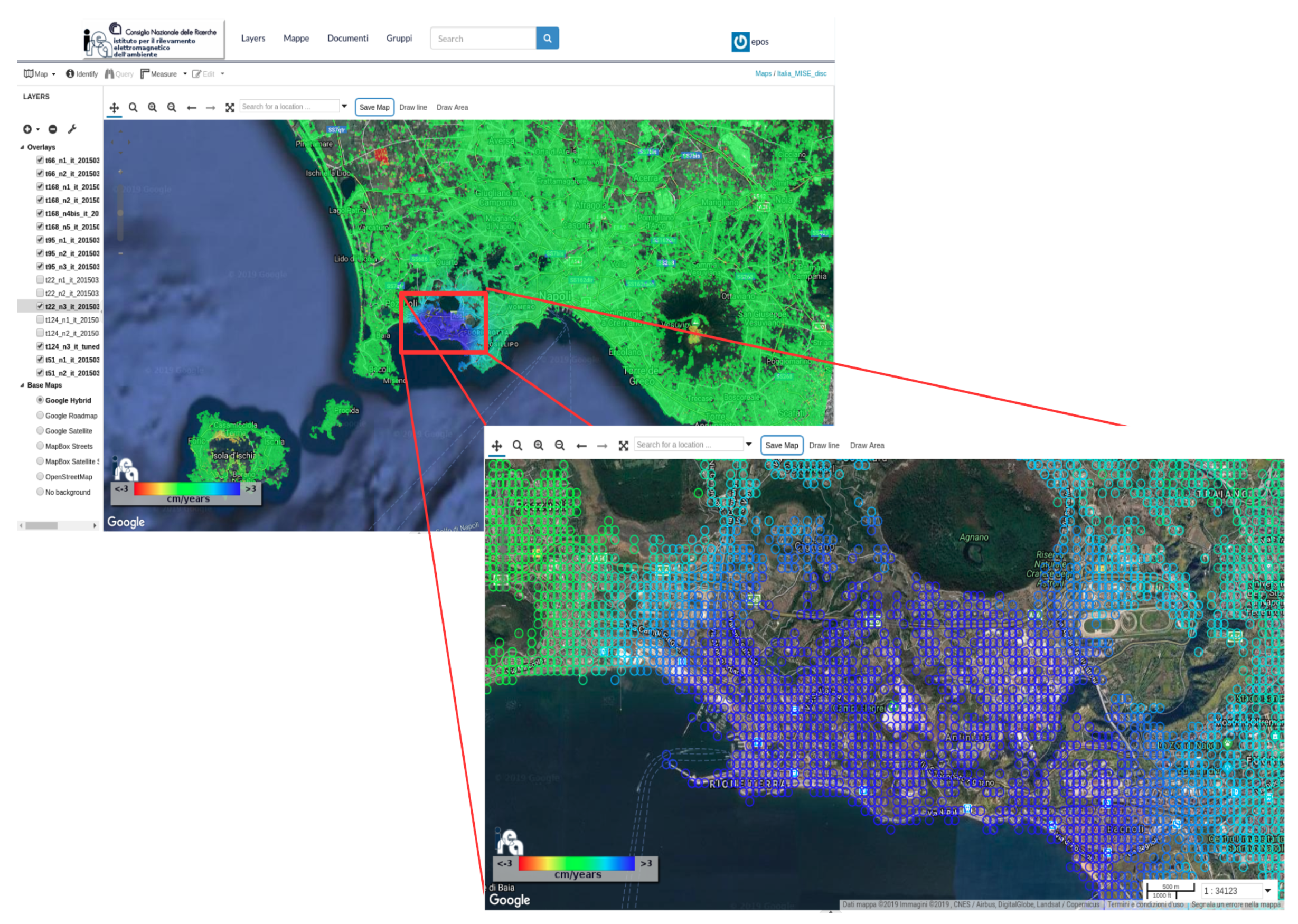
• data visualization and integration from different sources, both stored on infrastructures and from services supplied from outside through the Web Map Service (WMS) [79], by using an integrated WebGis environment to build interactive maps.

Moreover, we remark that GeoNode is written in the Python language [80] and leverages on well-known and robust Open Source products, which are summarized in the following:

• DJango: a high-level Python Web framework [81], used to develop GeoNode;
• GeoServer: an open source software server written in Java [82] that allows users to share and edit geospatial data. Note that, by using open standards set forth by the Open Geospatial Consortium (OGC), GeoServer allows GeoNode for great flexibility in map creation and data sharing [83];
• pyCSW: an OGC CSW server [84] written in Python. Note that, in GeoNode, pyCSW provides a standards based metadata and catalogue component [85];
• GeoExplorer: a webGIS component for GeoNode [86];
• GeoWebCache: a Java web application used to cache map to accelerate and optimize map image delivery [87];
• PostgreSQL: an object-relational database, allowing efficient storage, query, and analysis of the location information [88];
• PostGIS: a spatial database extender for PostgreSQL object-relational database. It adds support for geographic objects allowing location queries to be run in the Structured Query Language (SQL), a standard language for storing, manipulating and retrieving data in databases [89].

In Figure 4, the interactions among the GeoNode core components is shown.

GeoNode allows users to upload vector data and raster data. Vector data are uploaded in a PostgreSQL/PostGIS geodatabase as Shape Files, whereas satellite imagery and other kinds of raster data are retained as GeoTIFFs in the storage device of the file system. The uploaded data are then exported to the webGIS component of GeoNode, GeoExplorer, through GeoServer, by using GeoWebCache to accelerate and optimize the delivery of the map images. Moreover, Geoserver allows the access to PostgreSQL/PostGIS geodatabase, not only by using GeoExplorer, but also through other third part OGC compliant softwares, as for example QGIS [90] or arcGIS [91], to visualize and interact with the data.

As soon as the upload is finished, the user can fill the metadata in order to allow an easy data searching and retrieval through the CSW (OGC Catalogue Service) by pyCSW.

Moreover, once the data have been uploaded, GeoNode lets the user search by geographic coordinates or via keywords, in order to create maps with GeoExplorer. Note that all the layers are automatically re-projected to web Mercator for maps display, making possible the use of different popular base layers like Open Street Map [92] or Google Satellite [93]. Accordingly, the GeoNode capabilities make this platform a perfect candidate to build up a SDI for managing, visualizing, and analysing DInSAR deformation time-series and the related products, and for their integration with other data sources. In this context we remark that one of the key problems related to an effective exploitation of the advanced DInSAR products is the efficient handling of the spatio/temporal characteristics of these data, which may reach significantly large volumes, thus requiring the devolpment of innovative tools with respect to the already existing ones.

In the next Section we describe the necessary changes in the GeoNode platform functionalities in order to efficiently exploit the results achieved through advanced DInSAR processing techniques.

However, before going into details of these modifications, let us provide some words on the reason way we focused on GeoNode. Indeed, various open source software tools are available for building SDIs but GeoNode appeared to us as the most appropriate choice because:

• it permits development of geospatial services within a fully free and open source framework;
• it is an environment originally developed to manage geographic content that easily allows the extension of its functionalities.

To clarify the impact of these issues let us refer to another platform, named Easy SDI [94], which has various features similar to GeoNode.

In this case our preference goes to GeoNode because of the following considerations:

• GeoNode uses as geodatabase PostgreSQL/PostGIS, developed into the free and open framework of the Open Source Geospatial Foundation (OSGeo) [95], while Easy SDI uses mySQL [96] which is owned by the Oracle Corporation [97];
• GeoNode is a dedicated environment to the SDIs development which is build in Django, an environment that allows the easy extension of the GeoNode functionalities by using Python codes. Instead, Easy SDI is developed as a plug-in of the Joomla [98] Content Management System (CMS), a system not originally developed to manage geographic contents.

4. GeoNode Modifications for the Advanced DInSAR Processing Results Integration

We have already mentioned in the previous Section that the GeoNode platform provides two data formats for the data upload: a vector data format (Shape Files) and a raster data format (GeoTIFF), both importable through a GeoNode web interface (developed with Django). In particular, the vector data are stored in a PostgreSQL/PostGIS geodatabase table [88,89].

Accordingly, as a step of our work, it is necessary to implement a procedure to efficiently upload the available advanced DInSAR processing results. In particular, in our case, the upload procedure takes as input the ASCII text files produced by the SBAS-DInSAR processing chain (see Figure 2), which follows the standards defined within the European Plate Observing System (EPOS) [99] of the European Strategy Forum on Research Infrastructure (ESFRI) [100].

These DInSAR data files, as shown in Figure 5, are divided in two parts: (1) an header, which contains the metadata with the general information on the applied algorithm and the parameters of the sensor from which the SAR raw data have been obtained; (2) a part which contains, in each row, the deformation time-series and the related products for each of the coherent pixels of the SAR image sequence, which are represented, in our case, by: latitude, longitude, topography, mean deformation velocity, coherence, direction cosines [99]. Note that the direction cosines allow projecting the east, north and vertical deformation components into the radar LOS direction. The uploading process is based on “cutting” the deformation data measurements contained in each of the text files into several portions and stored in concurrent mode into the PostgreSQL /PostGIS geodatabase tables. Therefore, the number of these tables represents the level of parallelism of the loading data process and their size varies depending on the number of coherent pixels stored in the text file. On the other hand, in order to be imported into Geoserver as a single layer, the different tables are grouped into a virtual table (view), whose relation schema is showed in

Table 1. Relation schema of the geodatabase table.

Attribute Name	Attribute Type	Description
ID	long integer	numeric identification of the pixel
PLOT button	string	link calling a PHP module to visualize the deformation time-series, as specified in more detail later in this Section
lat	float	pixel latitude
lon	float	pixel longitude
topo	float	pixel altitude
vel	float	pixel deformation velocity
cohe	float	pixel coherence
cose	float	east direction cosine
cosn	float	north direction cosine
cosu	float	up direction cosine
zYYYY_xxxx (1)	float	reference deformation value of the time-series
zYYYY_xxxx (2)	float	second deformation value of the time-series
⋮	⋮	⋮
zYYYY_xxxx (n)	float	nth deformation value of the time-series

. We highlight that the attribute name zYYYY_xxxx (i) in Table 1 is the ith date of the deformation time-series, where YYYY represents the year and xxxx the fraction of the year.

Note that, apart from the PLOT button, the other attributes represent the products related to each coherent pixel of the deformation time-series and their deformation measurements.

This uploading procedure is written in the PERL programming language [101] by using the PERL threads module [102] to speed up the process, assigning each task of table loading to a separate thread and exploiting the multi-core architecture of the modern computing systems (see Figure 6). We point out that a PERL thread is a flow of control through a program with a single execution point [103]. The choice of the PERL programming language was determined by the fact that it is an interpreted language optimized for scanning text files and extracting information from them. Moreover, PERL is extendable through the Comprehensive Perl Archive Network (CPAN) [104] modules, providing many powerful extensions to the standard library, such as, for example, DBI [105] for database interface and PERL threads modules that we have extensively used in this work.

We further remark that the deformation measurements are loaded into the PostgreSQL/PostGIS geodatabase as polygon centered at the SBAS-DInSAR coordinates for each pixel, with an area representing the average extension of the SAR pixel (see Figure 7). With this regard, we remark that for sake of simplicity these polygons have been deliberately selected as symmetric although they may be modified to account for the typically non symmetric characteristics of the SAR pixels [24].

After uploading the DInSAR data in the PostgreSQL/PostGIS geodatabase, the data are further imported in Geoserver, by using the Geoserver REST API [106], applying a customized Styled Layer Descriptor (SLD) [107] to the mean velocity deformation map in order to highlight, with a color palette, the mean deformation velocity values on the investigated area (see Figure 7).

We underline that in our case we assumed that the mean velocity is the key parameter to be shown because it well represents the average deforming behavior of the area but, in principle, a different product included in the metadata could be shown.

Moreover, an updating procedure to refresh the already existing layer in the geodatabase, has also been implemented. This is similar to the uploading procedure described above, with the distinctive feature that, in this case, a set of tables related to the area under investigation already exists. In particular, the adopted strategy for updating an existing layer consists in emptying the tables content related to the time-series information and modifying the table structure by adding new columns to store new deformation measurements. Considering that GeoNode provides permissions policy, the choice to empty the table content instead of cancelling the tables preserves the users permissions on the data.

The next step of the modified GeoNode platform is the data synchronization between the Geoserver and the GeoNode webGIS interface (GeoExplorer), by using the GeoNode Management Commands updatelayers [108] which is essential for the visualization of the uploaded DInSAR measurements. Indeed, the visualization process of these data is not trivial, due to their huge amount to be displayed. To overcome this issue we use GeoWebCache, a Java web application, to cache the generated map tiles in order to accelerate and optimize the map image delivery. In particularly, we specifically chose to build for each dataset all the tiles before the data visualization in the GeoNode webGIS interface, by using the GeoWebCache REST API [109] to boost the performance of the map visualization (see Figure 8).

Another very relevant aspect, that has been already mentioned in the previous sections, is that the analysis of the advanced DInSAR processing results requires not only a space, but also a time representation. Although the SDI structures via the WMTS protocol [110] support time-dimension for visualizing and querying temporal information, we had to implement a dedicated functionality in PHP due to the relation schema of the geodatabase table we designed, according to the peculiarity of the data to be handled (see Table 1). More specifically, as defined in Table 1, in the relation schema of the geodatabase table there are no attributes of date type, but each date of the deformation time-series is identified by an attribute name (zYYYY_xxxx (1), for instance). Accordingly, each attribute name, relevant to a date of the deformation time-series, is associated with one deformation value. The reason for this choice is that it allows us to have any pixel represented by a single row of the geodatabase table. Moreover, this also allows us to dynamically update the table adding new columns in case new dates are added to the deformation time-series.

Specifically, in order to plot and over-plot graphs of the DInSAR deformation time-series relative to pixels belonging to the same layer or to different layers, we developed a PHP module based on the open source pChart library [111]. Accordingly, for each measurement pixel it has been added a plot button in the geodatabase record, which is nothing more that a link calling the PHP module to visualize the deformation time-series. Note that, the choice of using a link in each record of geodatabase has the advantage to visualize information by using different GIS clients, without developing a specific plug-in for each GIS client (see Figure 9).

Finally, two GeoNode webGIS plug-in have been also implemented, one to plot cross-sections of the mean deformation velocity layers (see Figure 10) and the other to download data from a selected area (see Figure 11). Both of these plug-in have been inserted in the map section of the GeoNode code and they permit us to retrieve information directly from the map, showing a pop-up with the list of intersected layers. Concerning the cross-sections plug-in, we highlight that it is possible to select one layer or more layers for which the spatial information of the mean deformation velocity have to be shown; instead, for the download plug-in it is possible to select only one layer at a time from which to download the pixel information included in the selected area. Both these routines are written in the Python Language and integrated in the section Map Code of GeoNode. This integration allows us to use the Django [81] framework for permissions management on the layers. Moreover, for the cross-section plug-in the open source library Bokeh [112] has also been used. Note that, the choice of a dedicated implementation of a web plug-in instead of using standard WPS [113] functionalities has been determined by the efficiency gained thanks to the direct access to geodatabase, which is even more relevant when considering the huge amount of data to be processed in our DInSAR scenario (multi-million pixels). In any case, we remark that a WPS service can be deployed as an alternative, less efficient—at the moment—solution.

5. Results

In order to demonstrate the effectiveness of the implemented extension of the GeoNode platform functionalities, we show in the following some examples relevant to the analysis of a DInSAR dataset of over all Italy.

In particular, we focus on the DInSAR time-series relevant to the acquisitions of the Sentinel-1 constellation, collected during the 2015–2018 time interval from descending orbits. Note that this dataset has been generated through the SBAS-DInSAR processing approach and is composed by 17 frames [77,78]. They have a maximum spatial extension of 56,000 km${}^2$ and are relevant to a temporal sequence of Sentinel-1 images ranging from a minimum number of 152 to a maximum one of 181. Let us start our analysis by considering Figure 12, where we show a synoptic view of the mean deformation velocity map over Italy relevant to the considered 17 SAR frames, represented on the latitude-longitude grid.

In addition, we show in Figure 13 some sample frames relevant to four selected zones composing the overall dataset of Figure 12. We remark that the DInSAR deformation results corresponding to each frame are included into txt files whose format has been shown in the previous Section (see Figure 5).

Considering that for the investigated case study each txt file corresponding to the multi-temporal DInSAR deformation information relevant to a single frame has an average size of 1.5 GB, the overall dataset dimension is approximately equal to 26 GB; they correspond to a total of 17 million SAR pixels and for each of these a deformation time-series and the related products are available.

We highlight that the average time needed to load in the PostgreSQL/PostGIS geodatabase the text file relevant to a selected frame is approximately 10 min. With this regard it is worth underlining that the DInSAR dataset loading, as well as the overall analysis presented in the following, is based on a mid-range performance server, characterized by an AMD Quad-Core Opteron TMProcessor 2356 architecture, equipped with 32 GB of RAM and a 5 TB disk configurated as a Linux software RAID5 with a storage extension of 11 TB. The Operating System (OS) used is the Ubuntu [114] distribution 14.04 LTS. The amount of disk storage for GeoWebCache and PostgreSQL/PostGIS geodatabase necessary for the creation of the interactive web map of Italy, is about 3 GB. We also remark that the exploited GeoWebCache architecture, as already discussed in Section 3 and Section 4, allows us to speed up the simultaneous display of all areas, making the map an interactive web-based consultation tool, compatible with OGC standards. Moreover, the temporal and spatial deformation information stored in the geodatabase as tables, are effectively loaded on the map of GeoNode webGIS interface by using the strategy to exploit pre-build tiles of size 256 × 256 pixels for each area and related zoom level (see Figure 8). Thanks to this strategy we may, for instance, very efficiently zoom in the different areas of the exploited DInSAR dataset, as for the case of the Campi Flegrei caldera (Southern Italy) shown in Figure 14.

In this case we may clearly see the coherent SAR pixels, each of which is represented on the ground by a polygon with an area of about 90 m × 90 m, whose color is associated with its mean velocity value. Note also that the area extension of each polygon is consistent with the SRTM DEM [115] used to geocode the DInSAR results.

Let us now show the implemented deformation time-series visualization functionality. To do this we consider the example shown in Figure 15, which is relevant to the deformation time-series of two selected pixels. The capability of visualizing multiple deformation time-series is evident as well as the possibility provided by the developed tool to automatically adapt the dynamic range in the y-direction in order to account for the different ranges of the considered time-series. Moreover, a similar capability has also been developed for the temporal scale represented by the x-axis of the available plots.

Subsequently, we present through Figure 16 the implemented functionality allowing us to visualize cross-sections of the mean deformation velocity information. Note that the abscissa of the plot refers to the distance expressed in kilometres of the points included in the considered cross-section segment; in this case the possibility of considering areas belonging to the different overlapping frames is also accounted for, because both the y- and x-axis are automatically scaled, depending on the DInSAR deformation velocities dynamic range and spatial extensions. Moreover, the coordinates, expressed in latitude and longitude, of the first and last pixel belonging to the traced segment are also automatically printed.

We further remark that the implemented time-series and cross-section deformation measurements visualization and analysis tools also allow us to straightforwardly save the corresponding data in the txt format shown in Figure 5. Similarly, it has been also implemented a functionality allowing us to save, in the already mentioned txt format, a portion of the overall DInSAR dataset, whose spatial extension can be a priori defined together with the overall preferences of the user account (see Figure 17).

We also underline that, an efficient procedure to save as “png” format image the content of the GeoNode webGIS component (GeoExplorer), has been implemented. The solution implemented a GeoExplorer plug-in, written in the JavaScript programming language [116] and using the html2canvas library [117], that makes a screen capture of the webGIS content, building the png image starting from the visualized tiles (see Figure 18). Note that, the implemented procedures allow us to avoid the high computational costs of the build-in GeoNode image generation procedure that makes the parsing of all the points composing the visualized area, which are stored as polygons in the PostgreSQL/PostGIS geodatabase.

As final example we show in Figure 19 the possibility to jointly analyze different data sources in addition to the uploaded DInSAR measurements. In particular, in this case we have overlapped to the mean deformation velocity map of Figure 12, the Italian municipalities seismic classification map relevant to the zone affected by the 2016–2017 seismic crisis in central Italy [118]. The multi-source data analysis capability provided by the extended version of the GeoNode platform is evident.

6. Discussion

SAR technology has already proven to be a key solution for monitoring wide areas of the Earth’s surface. In particular, the DInSAR techniques have demonstrated their capabilities to generate deformation maps and time-series suitable to detect, map and analyse the on-going surface displacement phenomena with centimetre to millimetre accuracy. Despite the huge range of applications developed in recent years, the operational use of DInSAR results obtained from the new generation satellite systems, such as the Sentinel-1 constellation, is hindered by the large amount of available measurements (note that the Sentinel-1 constellation already collects more than 10 TByte of data per day). Accordingly it is evident the need for developing advanced methodologies and techniques to handle such large DInSAR datasets of deformation maps and time-series. This work concerns the implementation of a SDI for managing, visualizing, analysing, and integrating with other data sources, large volumes of DInSAR results.

In particular, we focused on the GeoNode platform infrastructure which represents an excellent framework to implement a SDI and to extend the SDI functionalities in order to adapt them to our DInSAR-related requirements. More specifically, we underline that GeoNode:

(a)

permits development of geospatial services within a fully free and open source framework;

(b)

is an environment originally developed to manage geographic contents that easily allows the extension of its functionalities.

Moreover, as future perspectives, the use of a completely open source architecture like GeoNode gives us the possibility to distribute the developed codes under a GNU General Public Licence (GPL) [119]. In addition, a further improvement could be represented by the development of tools for animations relevant to the deformation time-series of a single pixel or for those of an area of interest.

We further remark that, since one of the most appreciated characteristics of GeoNode is the possibility to access to the data by using open standards endorsed by OGC (i.e., WMS and WFS for accessing maps and data and CSW as metadata catalogue), the proposed approach may contribute in paving the path to build a straightforward environment to find and share DInSAR data in an interoperable way and throughout multiple initiatives and projects, thus encouraging their reuse. Indeed, the available data can be offered through standard webservices, which are fundamental components of SDIs. We further remark that in the SDIs a particular attention is requested by metadata, an essential enabling factor for geospatial assets because discovery, retrieval, actual usage and re-use of data are tightly bound to the readability and quality of these descriptions. Like in many other use-cases, where geospatial metadata are often encoded in formats that are not aimed at easing searching and retrieval, also for the DInSAR data they are particularly difficult to be read and interpret, making more puzzling and boring the task of users who must fill metadata resources. To this purpose an open-source editing tool has been developed [120], which can be easily included in the overall architecture depicted in Figure 4 and in the flow chart of Figure 6, so that numeric metadata values in the DInSAR header can be made clear to generic users’ interpretation and users’ searching can be made more effective. These tasks are certainly worthy of future analysis.

7. Conclusions

In this paper we have presented the extension of the GeoNode platform functionalities in order to implement a SDI with the capability to effectively exploit DInSAR deformation time-series and their related products. In particular, the proposed implementation allows the users to efficiently investigate both the spatial and temporal characteristics of the DInSAR measurements, uploaded and updated in a PostgreSQL/PostGIS geodatabase which can reach a large data volume. Moreover, the capability of the modified platform to integrate DInSAR measurements with other data sources is straightforwardly achieved.

In particular, the implementation of the new GeoNode functionalities has been focused on the development of the following procedures:

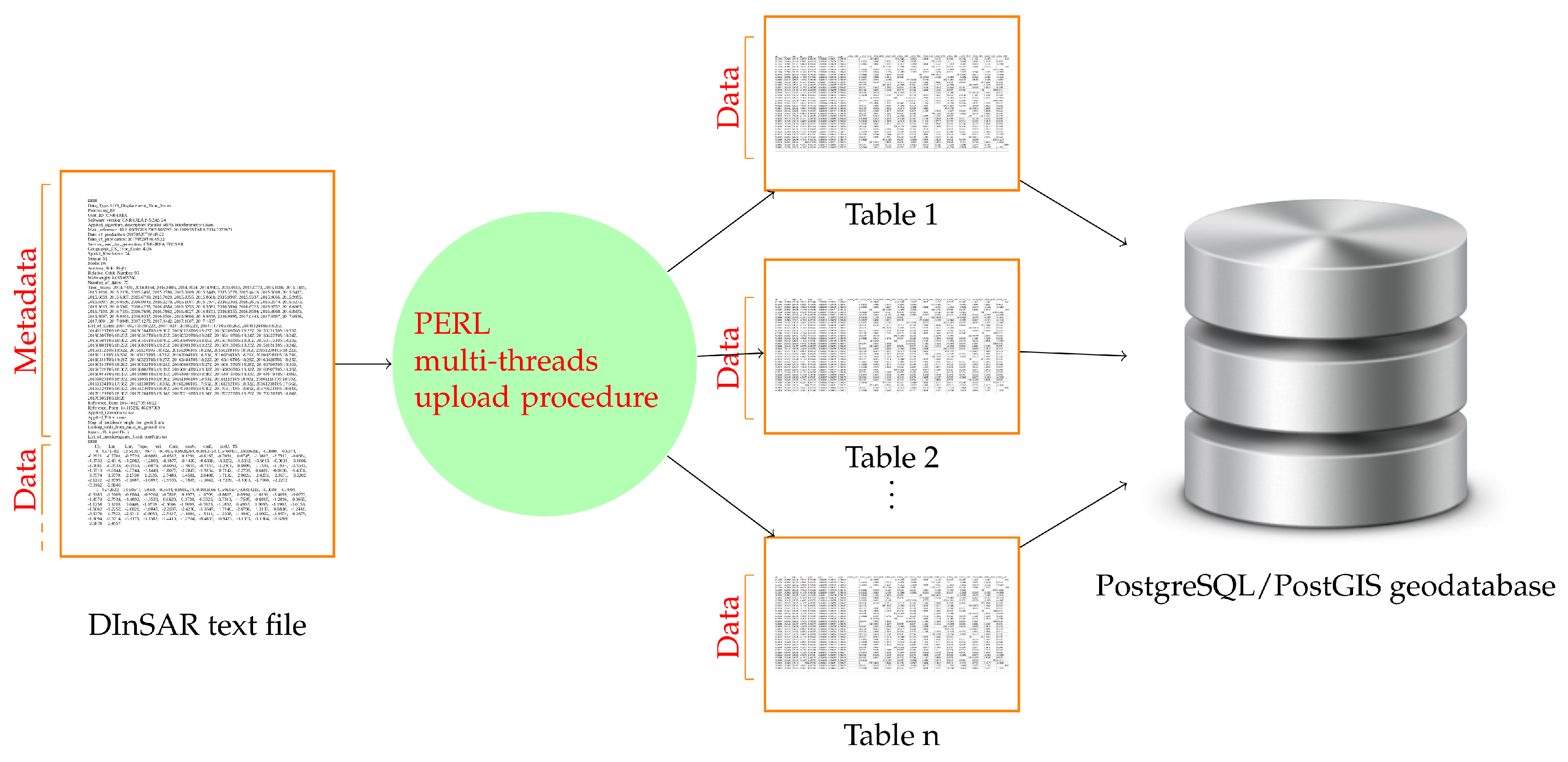
• upload/update of the DInSAR measurements in a PostgreSQL/PostGIS geodatabase;
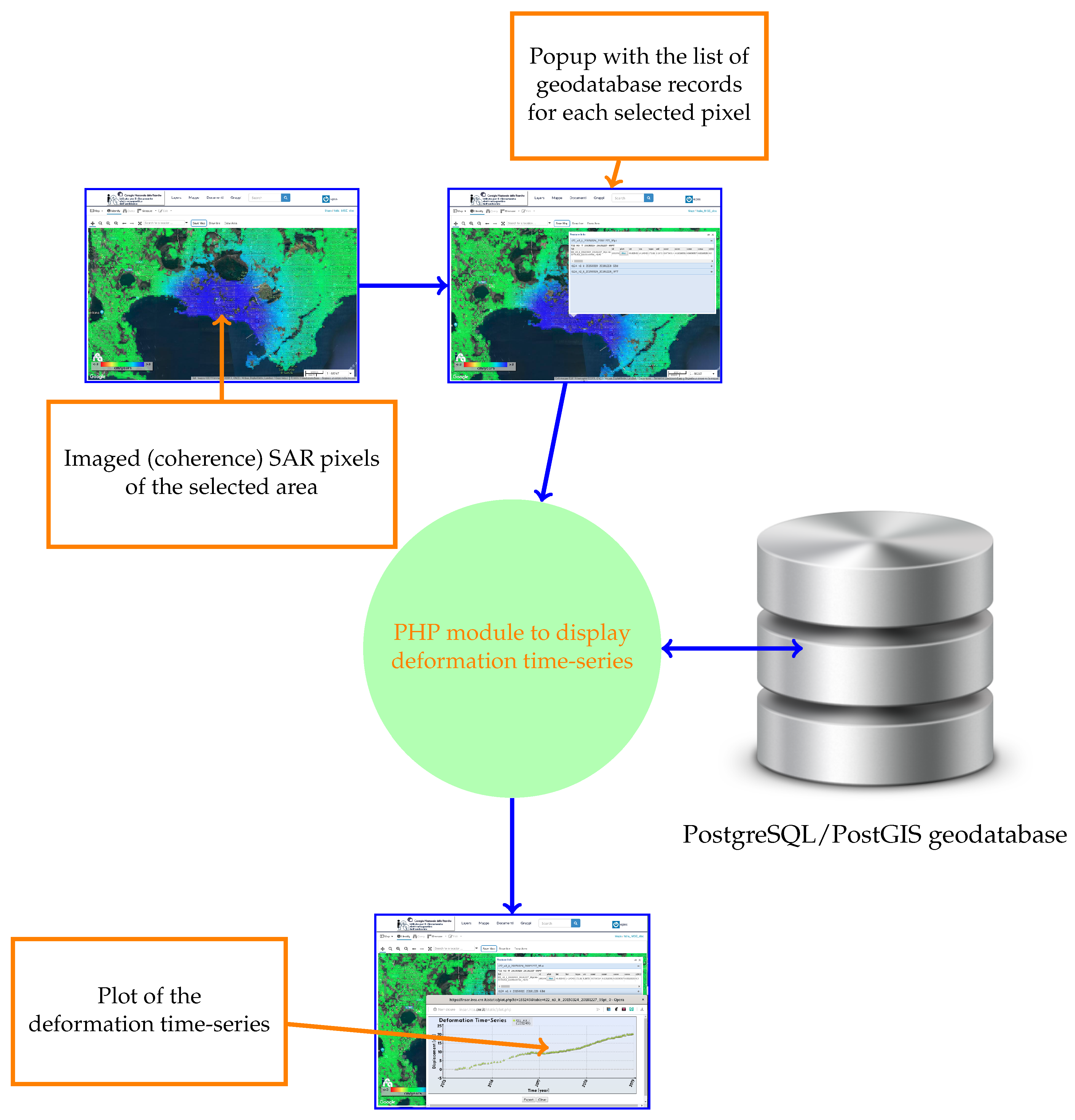
• visualization and analysis of the DInSAR deformation time-series, with the possibility to compare on the same graph the temporal evolution of multiple data pixels on different temporal spans belonging to the same processed dataset or to different ones;
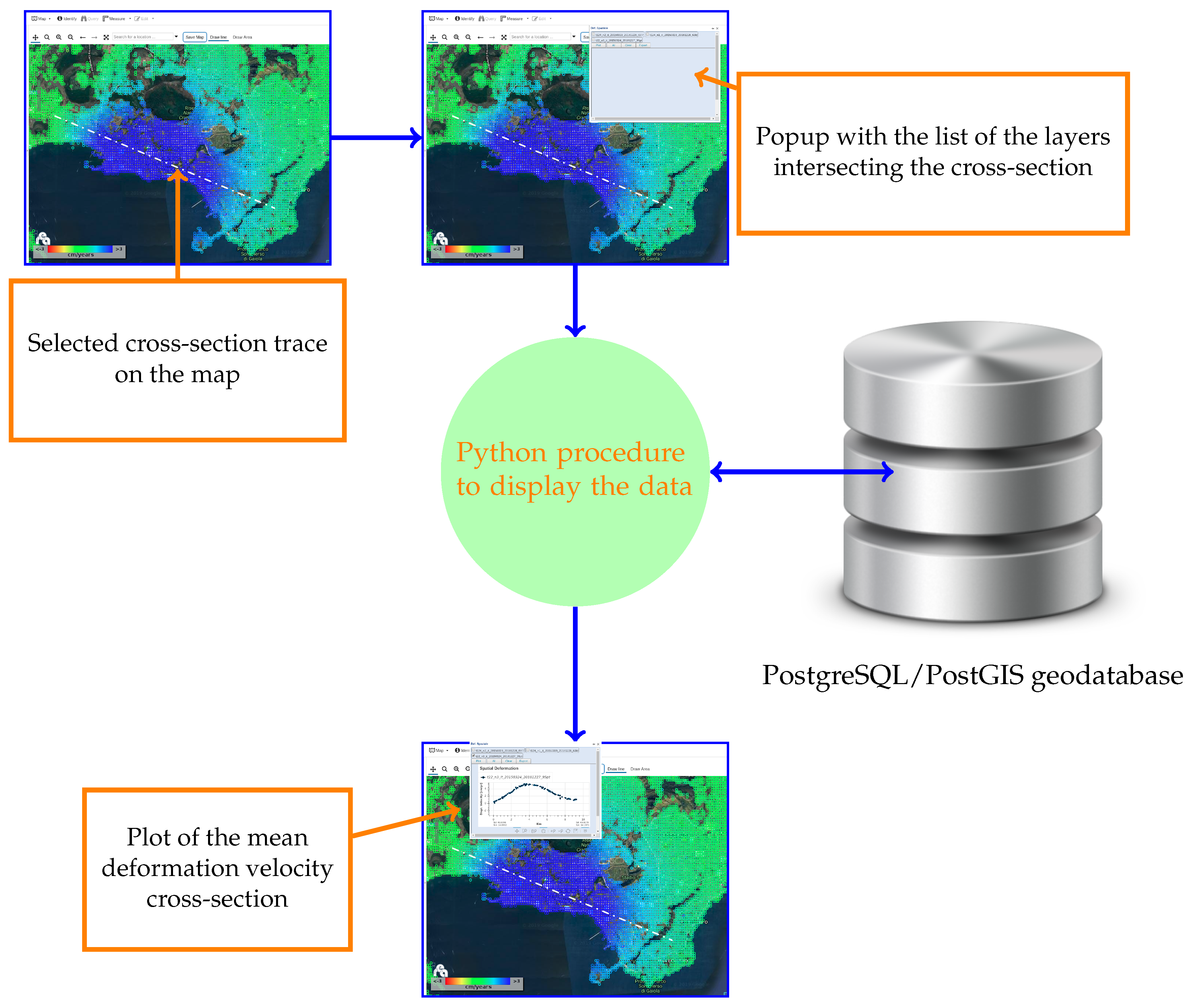
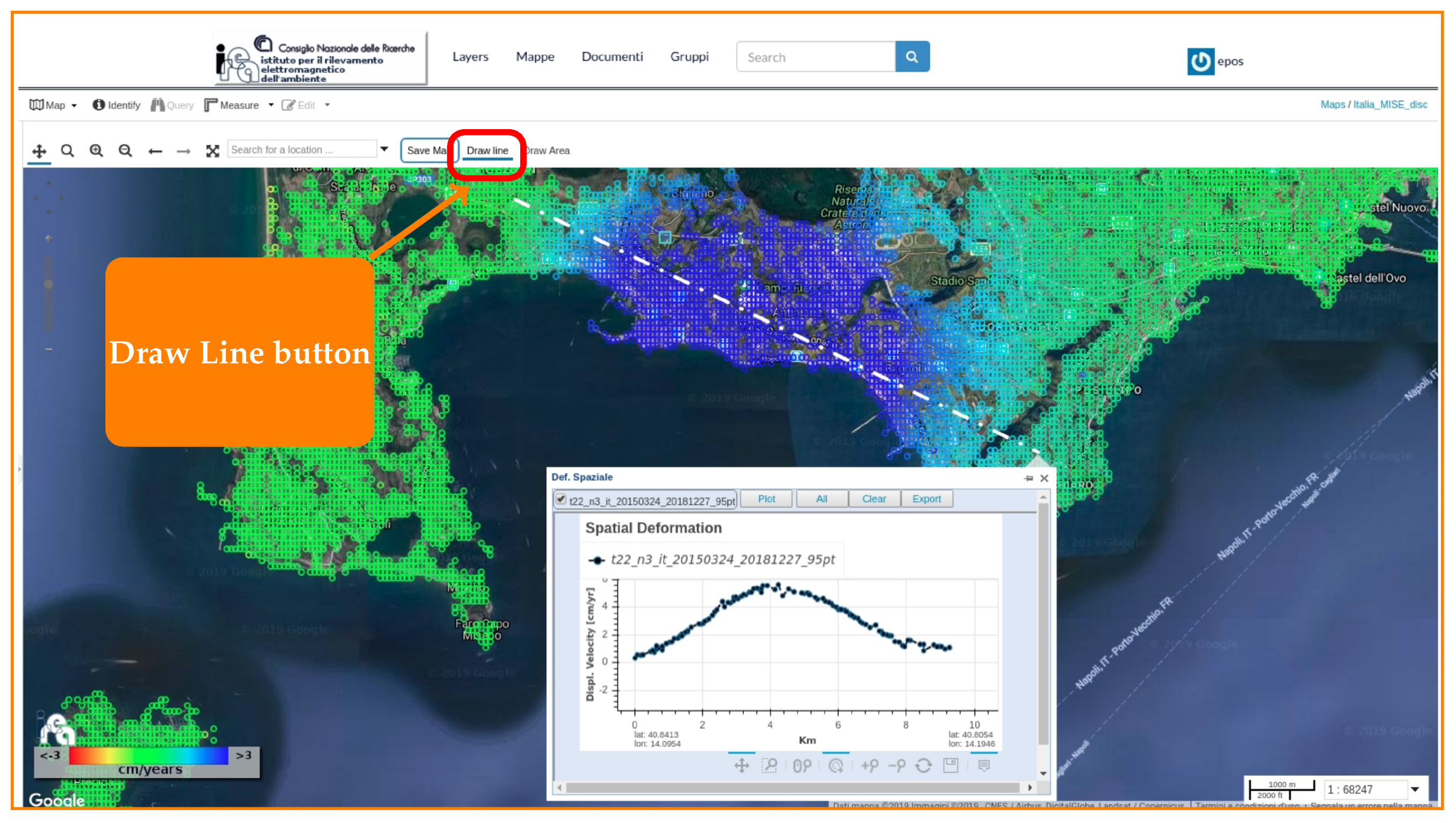
• visualization and analysis of the DInSAR mean deformation velocity cross-sections for each pixel belonging to a drawn segment on the map;
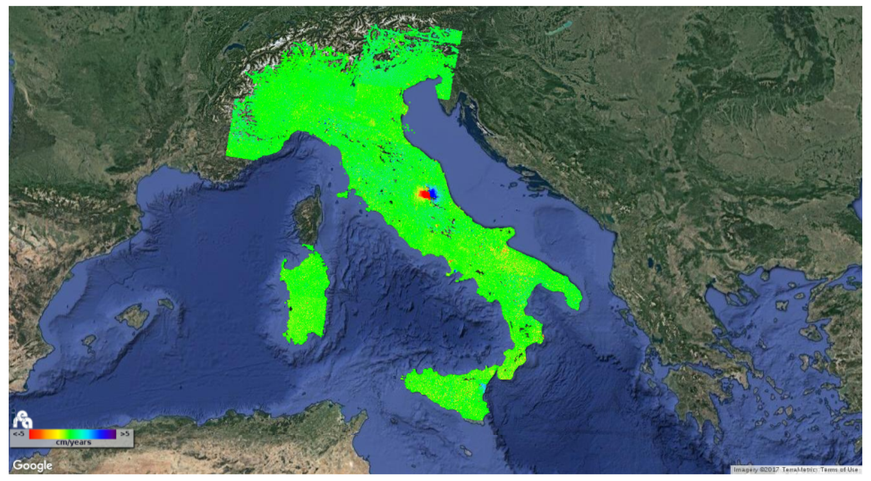
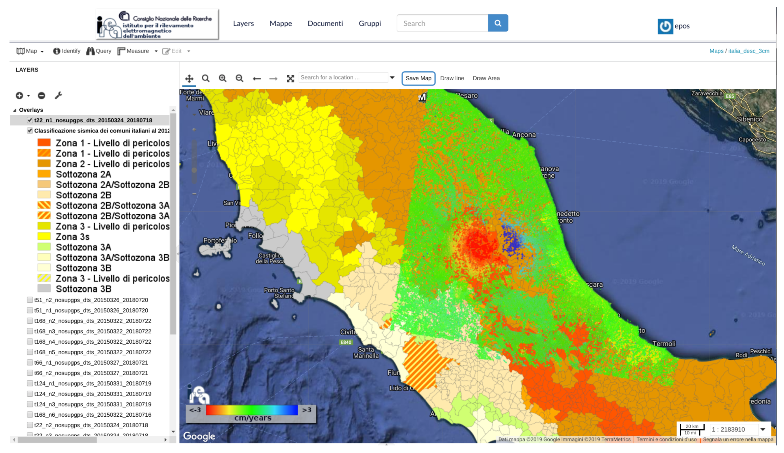
• visualization and analysis of the DInSAR mean deformation velocity maps;
• generation of a personalized color table (palette) for an appropriate visualization of the DInSAR mean deformation velocity values;
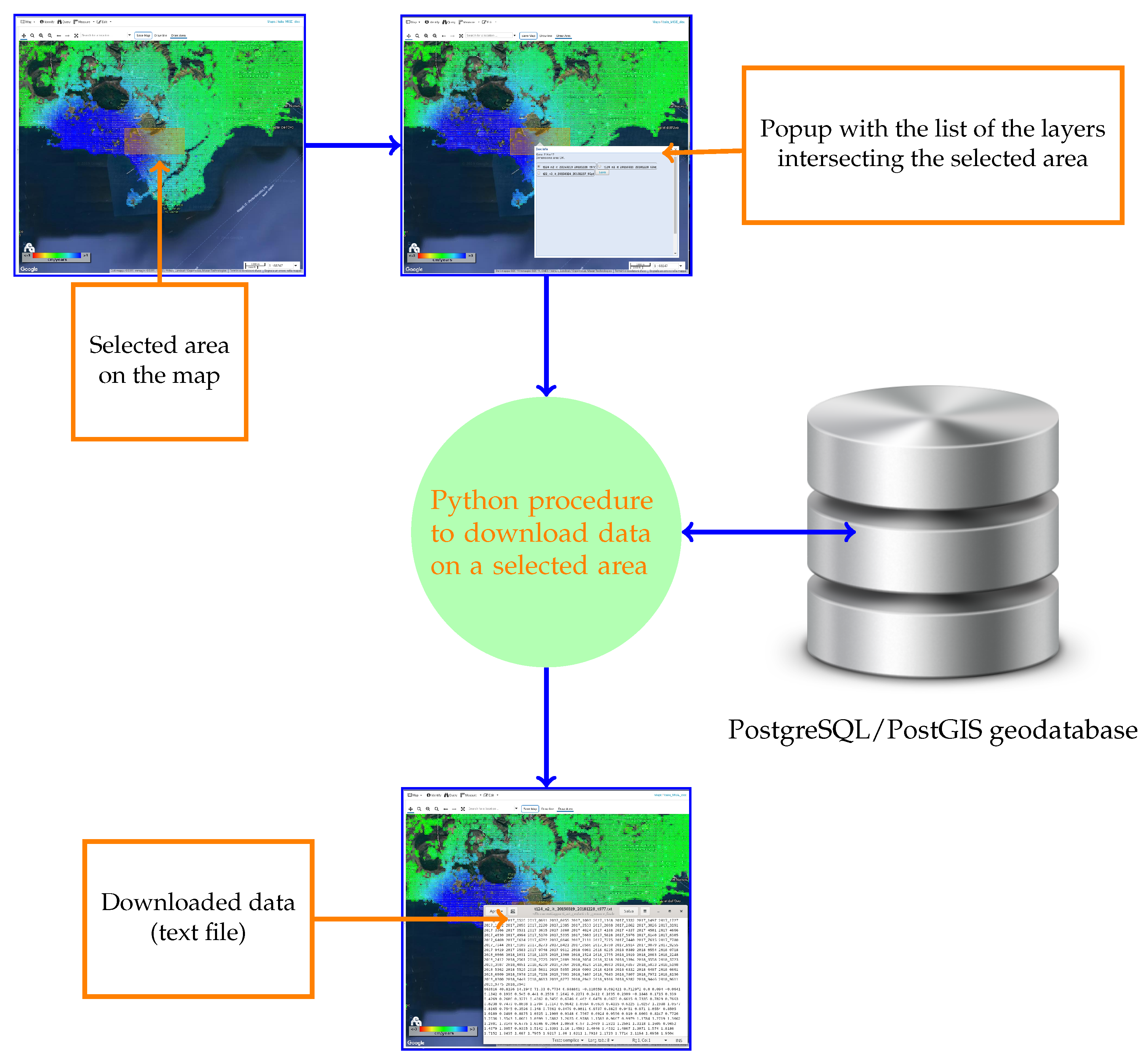
• download of data belonging to a selected area;
• creation of “png” format images to save the visualized layers in the GeoNode webGIS interface (GeoExplorer).

To demonstrate the effectiveness of the implemented extension of the GeoNode platform functionalities, results relevant to a Sentinel-1 DInSAR dataset of the Italian country have been extensively shown.

We find that the presented extension of the GeoNode platform, maintaining the original compliance with the OGC standards, can provide a useful contribution to the Big Data scenario which is characterizing the ongoing developments of the Earth Observation services.

References

1. VV.AA. 2019. Available online: https://business.esa.int/newcomers-earth-observation-guide (accessed on 31 July 2019).
2. Mathieu, P.P.; Borgeaud, M.; Desnos, Y.L.; Rast, M.; Brockmann, C.; See, L.; Kapur, R.; Mahecha, M.; Benz, U.; Fritz, S. The ESA’s Earth Observation Open Science Program [Space Agencies]. IEEE Geosci. Remote Sens. Mag. 2017, 5, 86–96. [Google Scholar] [CrossRef]
3. Borowitz, M. Open Space: The Global Effort for Open Access to Environmental Satellite Data; Information Policy; MIT Press: Cambridge, MA, USA, 2017. [Google Scholar]
4. Kiyoo, M. Relations between the eruptions of various volcanoes and the deformations of the ground surfaces around them. Earthq. Res. Inst. 1958, 36, 99–134. [Google Scholar]
5. Chinnery, M.A. The deformation of the ground around surface faults. Bull. Seismol. Soc. Am. 1961, 51, 355–372. [Google Scholar]
6. Massonnet, D.; Rossi, M.; Carmona, C.; Adragna, F.; Peltzer, G.; Feigl, K.; Rabaute, T. The displacement field of the Landers earthquake mapped by radar interferometry. Nature 1993, 364, 138–142. [Google Scholar] [CrossRef]
7. Massonnet, D.; Briole, P.; Arnaud, A. Deflation of Mount Etna monitored by spaceborne radar interferometry. Nature 1995, 375, 567. [Google Scholar] [CrossRef]
8. Peltzer, G.; Rosen, P. Surface Displacement of the 17 May 1993 Eureka Valley, California, Earthquake Observed by SAR Interferometry. Science 1995, 268, 1333–1336. [Google Scholar] [CrossRef]
9. Fialko, Y.; Simons, M.; Agnew, D. The complete (3-D) surface displacement field in the epicentral area of the 1999 MW7.1 Hector Mine Earthquake, California, from space geodetic observations. Geophys. Res. Lett. 2001, 28, 3063–3066. [Google Scholar] [CrossRef]
10. Cascini, L.; Ferlisi, S.; Fornaro, G.; Lanari, R.; Peduto, D.; Zeni, G. Subsidence monitoring in Sarno urban area via multi-temporal DInSAR technique. Int. J. Remote Sens. 2006, 27, 1709–1716. [Google Scholar] [CrossRef]
11. Colesanti, C.; Wasowski, J. Investigating landslides with space-borne Synthetic Aperture Radar (SAR) interferometry. Eng. Geol. 2006, 88, 173–199. [Google Scholar] [CrossRef]
12. Clough, R.; Woodward, R. Analysis of Embankment Stresses and Deformations; Soil Mechanics and Bituminous Materials Laboratory, University of California: Berkeley, CA, USA, 1966. [Google Scholar]
13. Yerkes, R.; Castle, R. Surface deformation associated with oil and gas field operations in the United States. Land Subsid. 1969, 1, 55–64. [Google Scholar]
14. Farrell, W.E. Deformation of the Earth by surface loads. Rev. Geophys. 1972, 10, 761–797. [Google Scholar] [CrossRef]
15. Orr, M., Jr. CO2 capture and storage: Are we ready? Energy Environ. Sci. 2009, 2, 449–458. [Google Scholar] [CrossRef]
16. O’Reilly, M.; New, B. Settlements above tunnels in the United Kingdom—Their magnitude and prediction. In Proc. Tunnelling ’82; Institution of Mining & Metallurgy: London, UK, 1982; pp. 173–181. [Google Scholar]
17. Hsieh, P.A. Deformation-Induced Changes in Hydraulic Head During Ground-Water Withdrawal. Groundwater 1996, 34, 1082–1089. [Google Scholar] [CrossRef]
18. Gourmelen, N.; Amelung, F.; Casu, F.; Manzo, M.; Lanari, R. Mining-related ground deformation in Crescent Valley, Nevada: Implications for sparse GPS networks. Geophys. Res. Lett. 2007, 34. [Google Scholar] [CrossRef] [Green Version]
19. Rackley, S.A. Carbon Capture and Storage; Butterworth-Heinemann: Oxford, UK, 2017. [Google Scholar]
20. Gabriel, A.K.; Goldstein, R.M.; Zebker, H.A. Mapping small elevation changes over large areas: Differential radar interferometry. J. Geophys. Res. Solid Earth 1989, 94, 9183–9191. [Google Scholar] [CrossRef]
21. Massonnet, D.; Feigl, K.L. Radar interferometry and its application to changes in the Earth’s surface. Rev. Geophys. 1998, 36, 441–500. [Google Scholar] [CrossRef]
22. Bürgmann, R.; Rosen, P.A.; Fielding, E.J. Synthetic Aperture Radar Interferometry to Measure Earth’s Surface Topography and Its Deformation. Annu. Rev. Earth Planet. Sci. 2000, 28, 169–209. [Google Scholar] [CrossRef]
23. Zebker, H.A.; Villasenor, J. Decorrelation in interferometric radar echoes. IEEE Trans. Geosci. Remote Sens. 1992, 30, 950–959. [Google Scholar] [CrossRef] [Green Version]
24. Franceschetti, G.; Lanari, R. Synthetic Aperture Radar Processing; CRC: Boca Raton, FL, USA, 1999. [Google Scholar]
25. Rosen, P.A.; Hensley, S.; Joughin, I.R.; Li, F.K.; Madsen, S.N.; Rodriguez, E.; Goldstein, R.M. Synthetic aperture radar interferometry. Proc. IEEE 2000, 88, 333–382. [Google Scholar] [CrossRef]
26. Ferretti, A.; Prati, C.; Rocca, F. Permanent scatterers in SAR interferometry. IEEE Trans. Geosci. Remote Sens. 2001, 39, 8–20. [Google Scholar] [CrossRef]
27. Werner, C.; Wegmuller, U.; Strozzi, T.; Wiesmann, A. Interferometric point target analysis for deformation mapping. In Proceedings of the IGARSS 2003 IEEE International Geoscience and Remote Sensing Symposium, Proceedings (IEEE Cat. No.03CH37477), Toulouse, France, 21–25 July 2003; Volume 7, pp. 4362–4364. [Google Scholar] [CrossRef]
28. Hooper, A.; Zebker, H.; Segall, P.; Kampes, B. A new method for measuring deformation on volcanoes and other natural terrains using InSAR persistent scatterers. Geophys. Res. Lett. 2004, 31. [Google Scholar] [CrossRef]
29. Berardino, P.; Fornaro, G.; Lanari, R.; Sansosti, E. A New Algorithm for Surface Deformation Monitoring Based on Small Baseline Differential SAR Interferograms. IEEE Trans. Geosci. Remote Sens. 2002, 40, 2375–2383. [Google Scholar] [CrossRef]
30. Mora, O.; Mallorqui, J.J.; Broquetas, A. Linear and nonlinear terrain deformation maps from a reduced set of interferometric SAR images. IEEE Trans. Geosci. Remote Sens. 2003, 41, 2243–2253. [Google Scholar] [CrossRef]
31. Lanari, R.; Mora, O.; Manunta, M.; Mallorquí, J.J.; Berardino, P.; Sansosti, E. A small baseline approach for investigating deformations on full resolution differential SAR interferograms. IEEE Trans. Geosci. Remote Sens. 2004, 42, 1377–1386. [Google Scholar] [CrossRef]
32. Hooper, A. A multi-temporal InSAR method incorporating both persistent scatterer and small baseline approaches. Geophys. Res. Lett. 2008, 35. [Google Scholar] [CrossRef] [Green Version]
33. Ferretti, A.; Fumagalli, A.; Novali, F.; Prati, C.; Rocca, F.; Rucci, A. A New Algorithm for Processing Interferometric Data-Stacks: SqueeSAR. IEEE Trans. Geosci. Remote Sens. 2011, 49, 3460–3470. [Google Scholar] [CrossRef]
34. Sansosti, E.; Berardino, P.; Bonano, M.; Calò, F.; Castaldo, R.; Casu, F.; Manunta, M.; Manzo, M.; Pepe, A.; Pepe, S.; et al. How second generation SAR systems are impacting the analysis of ground deformation. Int. J. Appl. Earth Obs. Geoinf. 2014, 28, 1–11. [Google Scholar] [CrossRef] [Green Version]
35. Copernicus. 2019. Available online: https://www.copernicus.eu/ (accessed on 31 July 2019).
36. Torres, R.; Snoeij, P.; Geudtner, D.; Bibby, D.; Davidson, M.; Attema, E.; Potin, P.; Rommen, B.; Floury, N.; Brown, M.; et al. GMES Sentinel-1 mission. Remote Sens. Environ. 2012, 120, 9–24. [Google Scholar] [CrossRef]
37. VV.AA. SDI Cookbook; Technical Report; Global Spatial Data Infrastructure Association: Gilbertville, IA, USA, 2012. [Google Scholar]
38. The White House; Office of Management and Budget (OMB). Circular No. A-16 Revised; 19 August 2002; Office of Management and Budget, US Government: Executive Office of the President of the United States: Washington, DC, USA, 2002.
39. VV.AA. 2019. Available online: https://www.opengeospatial.org/ (accessed on 31 July 2019).
40. VV.AA. 2019. Available online: http://interoperability-definition.info/en/ (accessed on 31 July 2019).
41. VV.AA. 2019. Available online: https://www.opengeospatial.org/ogc/glossary/i (accessed on 31 July 2019).
42. VV.AA. 2019. Available online: https://researchguides.library.wisc.edu/c.php?g=178144&p=1169699 (accessed on 31 July 2019).
43. VV.AA. 2019. Available online: http://geonode.org/ (accessed on 31 July 2019).
44. Elachi, C.; Geoscience, I.; Society, R.S. Spaceborne Radar Remote Sensing: Applications and Techniques; IEEE Press: New York, NY, USA, 1987. [Google Scholar]
45. Curlander, J.C.; McDonough, R.N. Synthetic Aperture Radar—Systems And Signal Processing; John Wiley & Sons, Inc.: Hoboken, NJ, USA, 1991. [Google Scholar]
46. Cumming, I.; Wong, F. Digital Processing of Synthetic Aperture Radar Data: Algorithms and Implementation; Artech House: Boston, MA, USA, 2005. [Google Scholar]
47. Rignot, E. Radar interferometry detection of hinge-line migration on Rutford Ice Stream and Carlson Inlet, Antarctica. Ann. Glaciol. 1998. [Google Scholar] [CrossRef]
48. Tesauro, M.; Berardino, P.; Lanari, R.; Sansosti, E.; Fornaro, G.; Franceschetti, G. Urban subsidence inside the city of Napoli (Italy) Observed by satellite radar interferometry. Geophys. Res. Lett. 2000, 27, 1961–1964. [Google Scholar] [CrossRef]
49. Hanssen, R. Radar Interferometry: Data Interpretation and Error Analysis (Remote Sensing and Digital Image Processing); Springer: Dordrecht, The Netherlands, 2006. [Google Scholar]
50. Lanari, R.; De Natale, G.; Berardino, P.; Sansosti, E.; Ricciardi, G.P.; Borgstrom, S.; Capuano, P.; Pingue, F.; Troise, C. Evidence for a peculiar style of ground deformation inferred at Vesuvius volcano. Geophys. Res. Lett. 2002, 29, 6-1–6-4. [Google Scholar] [CrossRef]
51. Manzo, M.; Ricciardi, G.; Casu, F.; Ventura, G.; Zeni, G.; Borgström, S.; Berardino, P.; Gaudio, C.D.; Lanari, R. Surface deformation analysis in the Ischia Island (Italy) based on spaceborne radar interferometry. J. Volcanol. Geotherm. Res. 2006, 151, 399–416. [Google Scholar] [CrossRef]
52. Lanari, R.; Zeni, G.; Manunta, M.; Guarino, S.; Berardino, P.; Sansosti, E. An integrated SAR/GIS approach for investigating urban deformation phenomena: A case study of the city of Naples, Italy. Int. J. Remote Sens. 2004, 25, 2855–2867. [Google Scholar] [CrossRef]
53. Perrone, A.; Zeni, G.; Piscitelli, S.; Pepe, A.; Loperte, A.; Lapenna, V.; Lanari, R. Joint analysis of SAR interferometry and electrical resistivity tomography surveys for investigating ground deformation: The case-study of Satriano di Lucania (Potenza, Italy). Eng. Geol. 2006, 88, 260–273. [Google Scholar] [CrossRef]
54. Fernández, J.; Tizzani, P.; Manzo, M.; Borgia, A.; González, P.J.; Martí, J.; Pepe, A.; Camacho, A.G.; Casu, F.; Berardino, P.; et al. Gravity-driven deformation of Tenerife measured by InSAR time series analysis. Geophys. Res. Lett. 2009, 36. [Google Scholar] [CrossRef] [Green Version]
55. Ruch, J.; Manconi, A.; Zeni, G.; Solaro, G.; Pepe, A.; Shirzaei, M.; Walter, T.R.; Lanari, R. Stress transfer in the Lazufre volcanic area, central Andes. Geophys. Res. Lett. 2009, 36. [Google Scholar] [CrossRef] [Green Version]
56. Hunstad, I.; Pepe, A.; Atzori, S.; Tolomei, C.; Salvi, S.; Lanari, R. Surface deformation in the Abruzzi region, Central Italy, from multitemporal DInSAR analysis. Geophys. J. Int. 2009, 178, 1193–1197. [Google Scholar] [CrossRef] [Green Version]
57. Manconi, A.; Walter, T.R.; Manzo, M.; Zeni, G.; Tizzani, P.; Sansosti, E.; Lanari, R. On the effects of 3-D mechanical heterogeneities at Campi Flegrei caldera, southern Italy. J. Geophys. Res. 2010, 115, B08405. [Google Scholar] [CrossRef]
58. Lanari, R.; Berardino, P.; Bonano, M.; Casu, F.; Manconi, A.; Manunta, M.; Manzo, M.; Pepe, A.; Pepe, S.; Sansosti, E.; et al. Surface displacements associated with the L’Aquila 2009 Mw 6.3 earthquake (central Italy): New evidence from SBAS-DInSAR time series analysis. Geophys. Res. Lett. 2010, 37. [Google Scholar] [CrossRef]
59. Zeni, G.; Bonano, M.; Casu, F.; Manunta, M.; Manzo, M.; Marsella, M.; Pepe, A.; Lanari, R. Long-term deformation analysis of historical buildings through the advanced SBAS-DInSAR technique: The case study of the city of Rome, Italy. J. Geophys. Eng. 2011, 8, S1. [Google Scholar] [CrossRef]
60. Manzo, M.; Fialko, Y.; Casu, F.; Pepe, A.; Lanari, R. A Quantitative Assessment of DInSAR Measurements of Interseismic Deformation: The Southern San Andreas Fault Case Study. Pure Appl. Geophys. 2011, 166, 1–20. [Google Scholar] [CrossRef]
61. Calò, F.; Ardizzone, F.; Castaldo, R.; Lollino, P.; Tizzani, P.; Guzzetti, F.; Lanari, R.; Angeli, M.G.; Pontoni, F.; Manunta, M. Enhanced landslide investigations through advanced DInSAR techniques: The Ivancich case study, Assisi, Italy. Remote Sens. Environ. 2014, 142, 69–82. [Google Scholar] [CrossRef] [Green Version]
62. Zhao, Q.; Pepe, A.; Gao, W.; Lu, Z.; Bonano, M.L.; He, M.; Wang, J.; Tang, X. A DInSAR Investigation of the Ground Settlement Time Evolution of Ocean-Reclaimed Lands in Shanghai. IEEE J. Sel. Top. Appl. Earth Obs. Remote Sens. 2015, 8, 1–19. [Google Scholar] [CrossRef]
63. Notti, D.; Caló, F.; Cigna, F.; Manunta, M.; Herrera, G.; Berti, M.; Meisina, C.; Tapete, D.; Zucca, F. A User-Oriented Methodology for DInSAR Time Series Analysis and Interpretation: Landslides and Subsidence Case Studies. Pure Appl. Geophys. 2015, 172, 1–25. [Google Scholar] [CrossRef]
64. Diao, F.; Walter, T.R.; Solaro, G.; Wang, R.; Bonano, M.; Manzo, M.; Ergintav, S.; Zheng, Y.; Xiong, X.; Lanari, R. Fault locking near Istanbul: Indication of earthquake potential from InSAR and GPS observations. Geophys. J. Int. 2016, 205, ggw048. [Google Scholar] [CrossRef]
65. Scifoni, S.; Bonano, M.; Marsella, M.; Sonnessa, A.; Tagliafierro, V.; Manunta, M.; Lanari, R.; Ojha, C.; Sciotti, M. On the joint exploitation of long-term DInSAR time series and geological information for the investigation of ground settlements in the town of Roma (Italy). Remote Sens. Environ. 2016, 182, 113–127. [Google Scholar] [CrossRef]
66. Bonano, M.; Manzo, M.; Casu, F.; Manunta, M.; Lanari, R. DinSAR for the monitoring of cultural heritage sites. In Sensing the Past; Springer: Berlin/Heidelberg, Germany, 2017; pp. 117–134. [Google Scholar]
67. Solari, L.; Ciampalini, A.; Raspini, F.; Bianchini, S.; Zinno, I.; Bonano, M.; Manunta, M.; Moretti, S.; Casagli, N. Combined Use of C- and X-Band SAR Data for Subsidence Monitoring in an Urban Area. Geosciences 2017, 7, 21. [Google Scholar] [CrossRef]
68. Casu, F.; Manzo, M.; Lanari, R. A quantitative assessment of the SBAS algorithm performance for surface deformation retrieval from DInSAR data. Remote Sens. Environ. 2006, 102, 195–210. [Google Scholar] [CrossRef]
69. Bonano, M.; Manunta, M.; Pepe, A.; Paglia, L.; Lanari, R. From Previous C-Band to New X-Band SAR Systems: Assessment of the DInSAR Mapping Improvement for Deformation Time-Series Retrieval in Urban Areas. IEEE Trans. Geosci. Remote Sens. 2013, 51, 1973–1984. [Google Scholar] [CrossRef]
70. Golub, G.H.; Van Loan, C.F. Matrix Computations, 3rd ed.; Johns Hopkins University Press: Baltimore, MD, USA, 1996. [Google Scholar]
71. Manunta, M.; Marsella, M.; Zeni, G.; Sciotti, M.; Atzori, S.; Lanari, R. Two-scale surface deformation analysis using the SBAS-DInSAR technique: A case study of the city of Rome, Italy. Int. J. Remote Sens. 2008, 29, 1665–1684. [Google Scholar] [CrossRef]
72. Pepe, A.; Sansosti, E.; Berardino, P.; Lanari, R. On the generation of ERS/ENVISAT DInSAR time-series via the SBAS technique. IEEE Geosci. Remote Sens. Lett. 2005, 2, 265–269. [Google Scholar] [CrossRef]
73. Bonano, M.; Manunta, M.; Marsella, M.; Lanari, R. Long-term ERS/ENVISAT deformation time-series generation at full spatial resolution via the extended SBAS technique. Int. J. Remote Sens. 2012, 33, 4756–4783. [Google Scholar] [CrossRef]
74. ASI. 2019. Available online: https://www.asi.it/scienze-della-terra/cosmo-skymed/ (accessed on 31 July 2019).
75. DLR. 2019. Available online: https://www.dlr.de/dlr/en/desktopdefault.aspx/tabid-10377/565_read-436/#/gallery/350 (accessed on 31 July 2019).
76. De Zan, F.; Monti Guarnieri, A. TOPSAR: Terrain Observation by Progressive Scans. IEEE Trans. Geosci. Remote Sens. 2006, 44, 2352–2360. [Google Scholar] [CrossRef]
77. Manunta, M.; De Luca, C.; Zinno, I.; Casu, F.; Manzo, M.; Bonano, M.; Fusco, A.; Pepe, A.; Onorato, G.; Berardino, P.; et al. The Parallel SBAS Approach for Sentinel-1 Interferometric Wide Swath Deformation Time-Series Generation: Algorithm Description and Products Quality Assessment. IEEE Trans. Geosci. Remote Sens. 2019, 57, 1–23. [Google Scholar] [CrossRef]
78. Zinno, I.; Bonano, M.; Buonanno, S.; Casu, F.; De Luca, C.; Manunta, M.; Manzo, M.; Lanari, R. National Scale Surface Deformation Time Series Generation through Advanced DInSAR Processing of Sentinel-1 Data within a Cloud Computing Environment. IEEE Trans. Big Data 2019, 1. [Google Scholar] [CrossRef]
79. VV.AA. 2019. Available online: http://www.opengeospatial.org/standards/wms (accessed on 31 July 2019).
80. VV.AA. 2019. Available online: https://www.python.org/ (accessed on 31 July 2019).
81. VV.AA. 2019. Available online: https://www.djangoproject.com/ (accessed on 31 July 2019).
82. VV.AA. 2019. Available online: https://www.java.com/it/download/faq/whatis_java.xml (accessed on 31 July 2019).
83. VV.AA. 2019. Available online: http://geoserver.org/about/ (accessed on 31 July 2019).
84. VV.AA. 2019. Available online: https://www.opengeospatial.org/standards/cat (accessed on 31 July 2019).
85. VV.AA. 2019. Available online: https://pycsw.org (accessed on 31 July 2019).
86. VV.AA. 2019. Available online: http://93.187.166.52:8081/opengeo-docs/geoexplorer/index.html (accessed on 31 July 2019).
87. VV.AA. 2019. Available online: https://www.osgeo.org/projects/geowebcache/ (accessed on 31 July 2019).
88. VV.AA. 2019. Available online: https://www.postgresql.org/ (accessed on 31 July 2019).
89. VV.AA. 2019. Available online: http://postgis.net/ (accessed on 31 July 2019).
90. VV.AA. 2019. Available online: https://qgis.org/it/site/ (accessed on 31 July 2019).
91. VV.AA. 2019. Available online: https://www.arcgis.com/index.html (accessed on 31 July 2019).
92. VV.AA. 2019. Available online: https://www.openstreetmap.org/#map=6/42.088/12.564 (accessed on 31 July 2019).
93. VV.AA. 2019. Available online: https://www.google.com/maps/ (accessed on 31 July 2019).
94. VV.AA. 2019. Available online: http://www.easysdi.org (accessed on 31 July 2019).
95. VV.AA. 2019. Available online: https://www.osgeo.org (accessed on 31 July 2019).
96. VV.AA. 2019. Available online: https://www.oracle.com/it/MySQL/ (accessed on 31 July 2019).
97. VV.AA. 2019. Available online: https://www.oracle.com/index.html (accessed on 31 July 2019).
98. VV.AA. 2019. Available online: https://www.joomla.org (accessed on 31 July 2019).
99. European Research Infrastructure on Solid Earth. Available online: https://www.epos-ip.org/tcs/satellite-data (accessed on 31 July 2019).
100. VV.AA. 2019. Available online: http://www.esfri.eu/ (accessed on 31 July 2019).
101. VV.AA. 2019. Available online: https://www.perl.org/ (accessed on 31 July 2019).
102. VV.AA. 2019. Available online: https://perldoc.perl.org/threads.html (accessed on 31 July 2019).
103. VV.AA. 2019. Available online: https://perldoc.perl.org/perlthrtut.html (accessed on 31 July 2019).
104. VV.AA. 2019. Available online: hhttps://www.cpan.org/ (accessed on 31 July 2019).
105. VV.AA. 2019. Available online: https://dbi.perl.org/ (accessed on 31 July 2019).
106. VV.AA. 2019. Available online: https://docs.geoserver.org/stable/en/user/rest/ (accessed on 31 July 2019).
107. VV.AA. 2019. Available online: https://www.opengeospatial.org/standards/sld/ (accessed on 31 July 2019).
108. VV.AA. 2019. Available online: https://geonodegeonode.readthedocs.io/en/latest/tutorials/admin/admin_mgmt_commands/index.html (accessed on 31 July 2019).
109. VV.AA. 2019. Available online: https://docs.geoserver.org/stable/en/user/geowebcache/rest/index.html (accessed on 31 July 2019).
110. VV.AA. 2019. Available online: https://www.opengeospatial.org/standards/wmts (accessed on 31 July 2019).
111. VV.AA. 2019. Available online: http://www.pchart.net/ (accessed on 31 July 2019).
112. VV.AA. 2019. Available online: http://bokeh.pydata.org/ (accessed on 31 July 2019).
113. VV.AA. 2019. Available online: https://www.opengeospatial.org/standards/wps (accessed on 31 July 2019).
114. VV.AA. 2019. Available online: http://www.ubuntu.com/ (accessed on 31 July 2019).
115. NASA. 2019. Available online: https://www2.jpl.nasa.gov/srtm/ (accessed on 31 July 2019).
116. VV.AA. 2019. Available online: https://developer.mozilla.org/en-US/docs/Web/JavaScript/Reference (accessed on 31 July 2019).
117. Von Hertzen, N. 2017. Available online: https://html2canvas.hertzen.com/e (accessed on 31 July 2019).
118. Ministero dell’Ambiente e della Tutela del Territorio e del Mare. 2017. Available online: http://wms.pcn.minambiente.it/ogc?map=%2Fms_ogc%2FWMS_v1.3%2FVettoriali%2FClassificazione_sismica_2012.map (accessed on 31 July 2019).
119. VV.AA. 2019. Available online: https://www.gnu.org/licenses/licenses.en.html (accessed on 31 July 2019).
120. Fugazza, C.; Pepe, M.; Oggioni, A.; Tagliolato, P.; Pavesi, F.; Carrara, P. Describing Geospatial Assets in the Web of Data: A Metadata Management Scenario. ISPRS Int. J. Geo-Inf. 2016, 5, 229. [Google Scholar] [CrossRef]
Figure 1. Pictorial representation of the DInSAR scenario; note that in this case we are assuming the ideal case of subsequent acquisitions carried out from the same orbital path.
Remotesensing 11 02133 g001
Figure 2. The SBAS-DInSAR algorithm processing flow: from left to right, large number of SAR data are processed to generate a stack of interferograms with small temporal and spatial baselines, from which velocity deformation maps and deformation time-series are estimated.
Remotesensing 11 02133 g002
Figure 3. TOPS mode Sentinel-1 amplitude image of Italy; the 250 Km swath extension is highlighted.
Remotesensing 11 02133 g003
Figure 4. Flow chart of the GeoNode core components interactions.
Remotesensing 11 02133 g004
Figure 5. Sample text file showing the exploited DInSAR results data format; note that the metadata and deformation measurements are highlighted.
Remotesensing 11 02133 g005
Figure 6. Flow chart of the uploading information procedure.
Remotesensing 11 02133 g006
Figure 7. Polygons representing the imaged (coherent) SAR pixels; note that the color of each polygon is associated to its mean deformation velocity value. Moreover, in the highlighted squared rectangle the color palette is presented.
Remotesensing 11 02133 g007
Figure 8. Pictorial representation of the pre-build tiles for different levels of zoom.
Remotesensing 11 02133 g008
Figure 9. Flow chart of the deformation time-series plotting procedure.
Remotesensing 11 02133 g009
Figure 10. Flow chart of the mean deformation velocity cross-section plotting procedure.
Remotesensing 11 02133 g010
Figure 11. Flow chart of the procedure for download data on a selected area.
Remotesensing 11 02133 g011
Figure 12. Sentinel-1 DInSAR mean deformation velocity map of whole Italian territory uploaded to the extended GeoNode platform.
Remotesensing 11 02133 g012
Figure 13. Mean deformation velocity maps relevant to a selection of four frames of the overall DInSAR dataset shown in Figure 12 including the: (a) Lombardia, Emilia-Romagna, Veneto and Trentino Alto Adige Regions, (b) Marche, Umbria, Lazio, Abruzzo, Molise and Campania Regions, (c) Lazio, Campania, Abruzzo and Molise Regions, and (d) Sicily and Calabria Regions.
Remotesensing 11 02133 g013
Figure 14. Zoomed view of the Sentinel-1 SBAS-DInSAR mean deformation velocity map relevant to the Campi Flegrei caldera (Italy): each polygon represents an area on the ground of about 90 m × 90 m.
Remotesensing 11 02133 g014
Figure 15. Example of the implemented deformation time-series plot visualization and analysis functionality.
Remotesensing 11 02133 g015
Figure 16. Example of the implemented mean deformation velocity cross-sections visualization and analysis functionality.
Remotesensing 11 02133 g016
Figure 17. Example of the implemented download web plug-in on a selected area.
Remotesensing 11 02133 g017
Figure 18. Example of saving as "png" format image an area visualized in GeoExplorer; highlighted in the red rectangle is the Save Map button.
Remotesensing 11 02133 g018
Figure 19. Example of joint analysis of different data sources: overlap of the DInSAR mean deformation velocity (see Figure 10) and the Italian municipalities seismic classification [118] maps relevant to the zone affected by the 2016-2017 seismic crisis in central Italy.
Remotesensing 11 02133 g019