Classifications of Forest Change by Using Bitemporal Airborne Laser Scanner Data

Abstract

Changes in forest areas have great impact on a range of ecosystem functions, and monitoring forest change across different spatial and temporal resolutions is a central task in forestry. At the spatial scales of municipalities, forest properties and stands, local inventories are carried out periodically to inform forest management, in which airborne laser scanner (ALS) data are often used to estimate forest attributes. As local forest inventories are repeated, the availability of bitemporal field and ALS data is increasing. The aim of this study was to assess the utility of bitemporal ALS data for classification of dominant height change, aboveground biomass change, forest disturbances, and forestry activities. We used data obtained from 558 field plots and four repeated ALS-based forest inventories in southeastern Norway, with temporal resolutions ranging from 11 to 15 years. We applied the k-nearest neighbor method for classification of: (i) increasing versus decreasing dominant height, (ii) increasing versus decreasing aboveground biomass, (iii) undisturbed versus disturbed forest, and (iv) forestry activities, namely untouched, partial harvest, and clearcut. Leave-one-out cross-validation revealed overall accuracies of 96%, 95%, 89%, and 88% across districts for the four change classifications, respectively. Thus, our results demonstrate that various changes in forest structure can be classified with high accuracy at plot level using data from repeated ALS-based forest inventories.

1. Introduction

Changes in land use and land cover have great implications on a range of ecosystem functions [1,2,3]. Particularly changes in forest areas have received considerable research attention in recent years, due to their impacts on biodiversity and carbon pools [4,5]. Resultantly, the development of reliable and timely systems for monitoring forest change across different spatial and temporal scales has become a central task in forestry. Primary motives have been the provision of data for national users such as government and conservation agencies, forest organizations and industries, and international reporting in accordance with treaties and conventions. Although forest changes typically are monitored in national programs [6,7] and reported at a national level, forest management decisions that directly induce those changes are made locally, namely at the level of municipalities, forest properties, and stands, i.e., treatment units. At such local scales, sampling rates of national monitoring programs are too low to obtain the necessary information [8], and local inventories are carried out to inform forest management.

Remote sensing provides a means to collect large amounts of information on forest attributes, and recent decades have witnessed substantial innovations in remote sensing technologies and data processing algorithms [9,10]. This has greatly facilitated the use of remotely sensed data for forest monitoring across various spatial and temporal scales. At global and national levels, coarse resolution optical satellite imagery provides useful information for estimating forest cover [11,12] and biomass [13,14]. At the level of forest properties and stands, high-resolution three-dimensional data have proven particularly useful for forest inventory applications [15]. Airborne laser scanning (ALS) provides accurate three-dimensional data on terrain surface and vegetation height, and in forest management inventories in numerous countries across the globe, it is common practice to use ALS data in estimating and mapping forest attributes [16] for local management needs.

ALS-based forest management inventories typically cover areas in the range of 100–1000 km² per project [17], in which forest attributes are commonly estimated and mapped using the area-based approach [18,19]. This approach involves developing statistical relationships between forest attributes and ALS metrics at the level of sample plots and predicting the attributes over a grid tessellating the entire inventory area into smaller cells. In stand-level forest inventories, model predictions for grid cells within stands are typically aggregated to obtain stand estimates. Alternatively, cell-level predictions can be used for wall-to-wall mapping of forest attributes [20], or as auxiliary information in probability-based sampling designs [21]. Parametric modeling techniques such as linear regression have widely been used due to their familiarity and practicality; however, they require assumptions regarding the distribution of the response variable, the model errors, and the absence of multicollinearity and autocorrelation. Because such assumptions may be violated in certain forest inventory applications for which remotely sensed data are used, nonparametric approaches have been studied extensively, such as nearest neighbor methods [22], regression trees [23], and neural networks [24]. Among these, nearest neighbor methods have become very popular in the field of forest inventory because they can easily be used for a wide range of applications, including classification, univariate and multivariate prediction, imputation, mapping, and inference [25].

The availability of multitemporal ALS data is increasing as ALS-based forest inventories are repeated through multiple cycles. Bitemporal ALS data have proven useful for estimating forest height growth [26,27] and aboveground biomass (AGB) change [28,29,30]. Although the quantification of changes in the mentioned attributes is highly relevant for forest planning, many applications in forestry require classification into discrete categories. Categorical variables such as dominant tree species, forest development class, and forest productivity have long been fundamental in forest planning. As ALS-based forest inventories are starting to be repeated in many countries, possibilities for new classification systems emerge that allow for temporal change monitoring.

A range of forest inventory applications may benefit from change classification. First, recent studies have shown that canopy height growth as depicted by bitemporal ALS data enables the estimation of forest productivity [31,32,33]. Forest productivity is among the most essential variables in forest management and is expensive to record in field surveys. The estimation of forest productivity requires the height of dominant trees (Hdom) to have increased during the observation period, as forest productivity would be underestimated in cases where Hdom growth has been disrupted. This calls for a classification of forest into positive and negative Hdom development prior to the estimation of forest productivity itself. Second, AGB change classes can be used as post-strata in AGB change estimation [34], and changes can be projected spatially to identify areas where changes have occurred, their spatial extents alone being relevant reporting units. Third, forest disturbance events such as storm damage and harvest have gained relevance due to their impacts on forest ecosystems [35,36,37,38] and carbon balances [30,39]. Finally, classification of forestry activities such as untouched, partial harvest, and clearcut are crucial for estimating and reporting net forest carbon fluxes, given that carbon emissions and removals must be attributed to certain offset activities [34].

Previous research has shown that single-date ALS data can be used to indicate past forest disturbances and silvicultural operations. For example, d’Oliveira et al. [40] used structural ALS metrics over a tropical forest in Brazil to identify selective logging. Other studies using single-date ALS data discriminated between forest development classes [41,42,43] and forest/non-forest classes for the purpose of stand delineation [44,45,46]. To monitor changes in forest structure over time, however, multitemporal data are needed. Bitemporal ALS data have been used to identify single harvested trees [47] and monitor canopy gap dynamics [48,49,50]. Næsset et al. [34] used bitemporal ALS data with a temporal resolution of 11 years to classify untouched, partial harvest, and clearcut forest at plot-level in a boreal forest in southeastern Norway using multinomial logistic regression. To the best of our knowledge, however, no further research has been done on the use of multitemporal ALS data for forest change classification. Here, we present the first study assessing the use of bitemporal ALS data for classification of various changes in forest structure. We used data acquired as part of repeated operational inventories carried out by a forest owner’s cooperative and demonstrated how such data can be used for local forest change monitoring.

The objective of this study was to assess the utility of bitemporal ALS data for classification of Hdom change, AGB change, forest disturbances and forestry activities. We distinguished between the following change classes: (i) increasing versus decreasing Hdom, (ii) increasing versus decreasing AGB, (iii) undisturbed versus disturbed forest and (iv) forestry activities namely untouched, partial harvest and clearcut.

2. Material and Methods

2.1. Study Areas

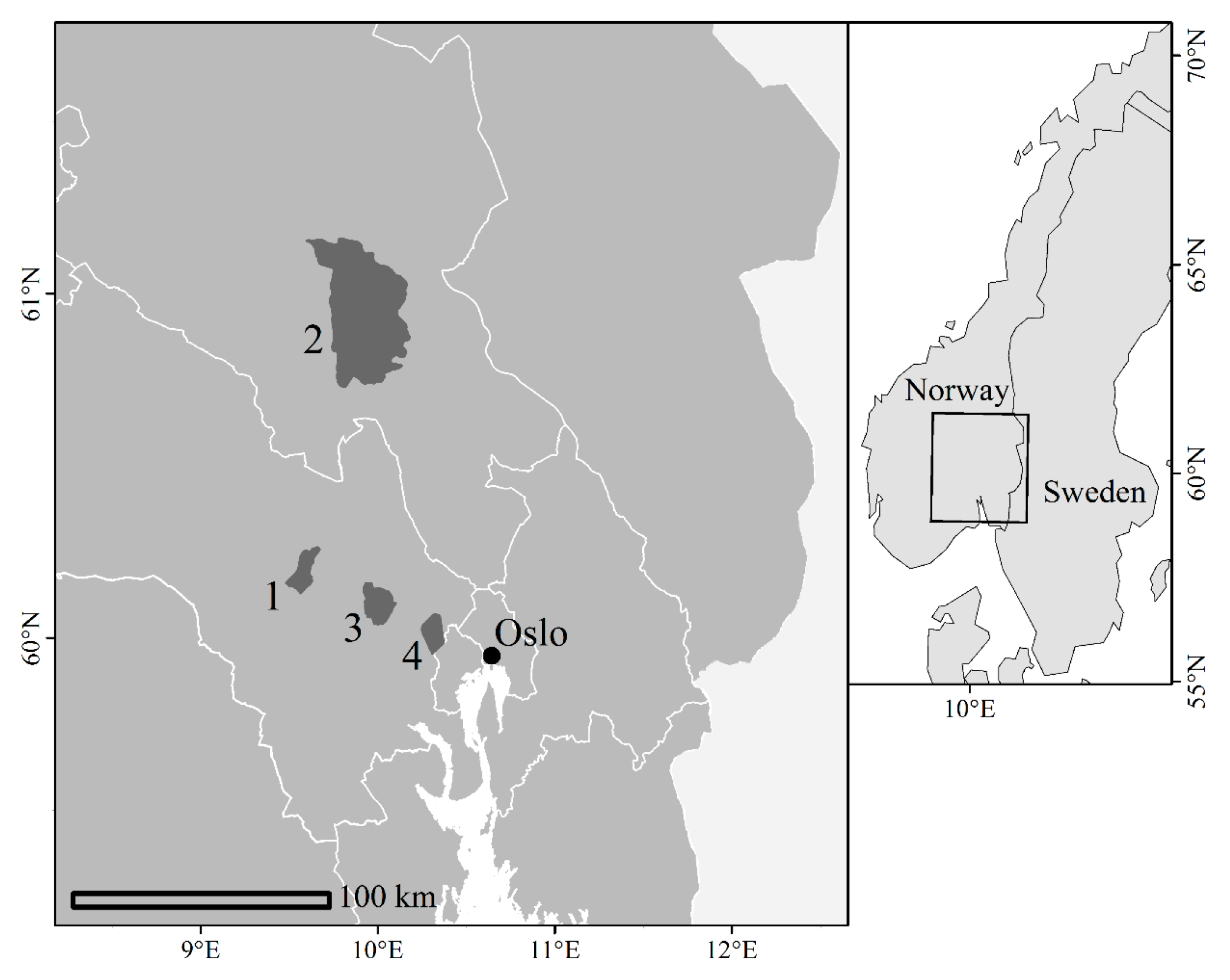
We used bitemporal field and ALS data acquired as part of four repeated forest inventories in southeastern Norway (Figure 1). The inventories were carried out by Viken Skog SA, a Norwegian forest owner’s cooperative, and were among the first commercial ALS-based trials in the early 2000s [17]. They were also among the first repeated ALS-based inventories. District 1 was part of the municipality of Krødsherad (60°10′N 9°35′E, 130–660 m above sea level) and comprised about 5000 ha productive forest [51]. The dominant tree species in the area are Norway spruce (Picea abies (L.) Karst.) and Scots pine (Pinus sylvestris L.). District 2 comprised about 49,000 ha productive forest in the municipality of Nordre Land (60°50′N 10°5′E, 140–900 m above sea level) [52], also mainly composed of Norway spruce and Scots pine. District 3, the district of Tyristrand (60°6′N 10°2′E, 150–480 m above sea level), comprised about 13,000 ha productive forest where Scots pine is the main species [17]. Lastly, District 4 was part of the municipality of Hole (60°1′N 10°20′E, 240–540 m above sea level) which comprises 6500 ha productive forest, dominated by Norway spruce [53].

2.2. Field Data

During the first inventory cycle (t₁), circular sample plots were distributed systematically throughout the districts by means of systematic stratified sampling designs. The sample plots had a radius of 8.61 m for district 1 and 8.92 m for the remaining districts, resulting in plot sizes of 233 m² and 250 m², respectively (

Table 1. Summary of the inventories and number of plots within forest development classes.

District	Name	Plot Size (m2)	First Inventory Cycle			Second Inventory Cycle
			Year	No. of Plots, Development Class * 2	No. of Plots, Development Classes 3–5	Year	No. of Plots, Development Class 2	No. of Plots, Development Classes 3–5
1	Krødsherad	233	2001	39	111	2016	19	131
2	Nordre Land	250	2003	0	198	2017	21	177
3	Tyristrand	250	2006	0	111	2017	3	108
4	Hole	250	2005	0	99	2017	12	87

* development class 2 = regeneration forest, class 3 = young forest, class 4 = mature forest, class 5 = forest ready for harvest.

). These are typical plot sizes in Norwegian operational forest inventories [54]. Stratification was carried out according to dominant tree species, site productivity, and forest development class as interpreted from aerial images, for details see [17,51,52,53]. In Norway, development classes represent the succession of production forest [55], where class 1 represents clear-felled stands, class 2 represents regeneration forests, typically with a height <10 m, class 3 represents young forest, class 4 represents mature forest, and class 5 represents forest ready for harvest. Development class 1 was omitted from the inventories, and at t₁, development class 2 was only included in the inventory of district 1. During the second inventory cycle (t₂), all plots were revisited, and they were remeasured unless a final harvest recently had taken place. For plots that had been subject to final harvest, those for which sufficient time had passed for regeneration to occur were remeasured if the regenerated forest had reached a height >0.5 m. Table 1 provides an overview of the inventories and the number of plots within forest development classes.

2.3. Plot Positioning

At t₁, plot center coordinates were determined using differential global navigation satellite systems (dGNSS) with Javad Legacy 20-channel receivers. The receivers measured pseudorange and carrier phase observables of the global positioning system (GPS) and the global navigation satellite system (GLONASS). A Javad Legacy served as a local base station. During post-processing, the coordinates were corrected against the collected reference data, and average accuracies of the planimetric plot center coordinates were <50 cm according to the positional standard errors reported by the Pinnacle 1.0 post-processing software. Plot centers were marked with wooden sticks. Upon revisiting the plots at t₂, a 226-channel Topcon HiPer SR was used in real-time kinematic mode to navigate to the plot centers. In case the wooden stick was not found, the position was remeasured using a Topcon Legacy E 40-channel receiver. During post-processing, the coordinates were corrected against reference data from the base stations of the Norwegian Mapping Authority using the software Magnet Tools [56].

2.4. Tree Measurements

On plots within forest development classes 3–5, the diameter at breast height (DBH) of trees exceeding given lower caliper limits was measured using a caliper during both inventory cycles. The lower caliper limits varied across districts and forest development classes, however on all plots, trees with a DBH ≥10 cm were calipered. For consistency, we excluded trees with a DBH <10 cm from the analysis across all districts and development classes. Furthermore, a sample of about 10 trees per plot was selected using a relascope and their heights were measured using a Vertex hypsometer.

On regeneration plots in district 1 and 2, four circular subplots of 40 m² were measured in cardinal directions from the plot center at a distance of 5.10 m. In district 3 and 4, three subplots of 40 m² were measured in north, southwest, and southeast directions at a distance of 5.35 m from the plot center. The radius around subplot centers was determined using a telescopic rod of 3.57 m. The subplots were divided into four quadrants in cardinal directions, and tree measurements were carried out within the separate quadrants. DBHs were not measured, as plot volumes were not calculated for regeneration plots in the inventories. The heights of the first tree in each quadrant, counting in a clockwise direction, and the first subjectively chosen dominant tree in each quadrant were measured using a height pole for trees with a height <8 m and a Vertex hypsometer for taller trees. A maximum of two dominant trees were selected in each quadrant.

2.5. Computation of Forest Attributes

Tree heights had only been measured for sample trees on plots of development classes 3–5. Thus, we estimated the heights of all calipered trees using a ratio estimator described in detail in Ørka et al. [57], based on the ratio between heights predicted with empirical DBH-height models and field-measured heights. We then computed Hdom as the mean predicted height of the trees corresponding to the largest 100 trees per ha, according to DBH [58]. Furthermore, we computed N as the number of calipered trees on each plot, scaled to a per hectare basis. Lastly, we predicted the AGB of individual trees using allometric models estimated by Marklund [59], and computed plot-level AGB as the sum of biomass predictions scaled to a per hectare basis.

For regeneration plots, we computed Hdom as the mean heights of dominant trees. We assumed values of AGB on regeneration plots to be negligible and thus zero. A summary of the computed field plot data is shown in Figure 2.

2.6. Field Data Classification

We assigned forest change classes to each plot according to changes in the computed forest attributes, dividing the plots into distinct change classes for the four classification schemes. The classification schemes were aimed at distinguishing between different changes in forest structure with increasing complexity. For classification of Hdom change, we discriminated between plots on which Hdom had increased and decreased during the observation period (

Table 2. Criteria for the classification schemes and numbers of plots within classes.

Classification	Class	Criteria *	No. of Plots
			District 1	District 2	District 3	District 4
Dominant height change	Increase	Hdomt2 > Hdomt1	118	165	99	83
	Decrease	All other plots	32	33	12	16
Aboveground biomass change	Increase	AGBt2 > AGBt1	118	148	81	79
	Decrease	All other plots	32	40	30	20
Forest disturbance	Undisturbed	Hdomt2 > Hdomt1 & AGBt2 > AGBt1 & Nt2 > 0.7×Nt1	75	149	68	77
	Disturbed	All other plots	75	49	43	22
Forestry activity	Untouched	Hdomt2 > Hdomt1 & AGBt2 > AGBt1 & Nt2 > 0.7×Nt1	75	149	68	77
	Partial harvest	Hdomt2 < Hdomt1 or AGBt2 < AGBt1 or Nt2 < 0.7×Nt1 & AGBt2 ≥ 0.1AGBt1	56	28	40	10
	Clearcut	Hdomt2 < Hdomt1 or AGBt2 < AGBt1 or Nt2 < 0.7×Nt1 & AGBt2 < 0.1AGBt1	19	21	3	12

* Hdom_t2 and Hdom_t1 = dominant height (m) during the second and first inventory cycles, respectively, AGB_t2 and AGB_t1 = aboveground biomass (Mg ha⁻¹) and, N_t2 and N_t1 = stem number (ha⁻¹), during the second and first inventory cycles, respectively.

). For classification of AGB change, the classes were defined as increased or decreased AGB. For the classification of forest disturbance, the classes were defined as undisturbed plots or disturbed plots, using changes in forest structure as proxies for disturbances. We applied the rule that a decrease in Hdom or AGB, or a reduction in N of at least 30% indicated that a disturbance had taken place during the observation period. Such reductions in forest attributes would rule out a natural succession and corresponding growth and mortality rates, and would therefore indicate that a substantial disturbance such as storm damage or thinning had occurred. For the classification of forestry activity, we further separated these changes by distinguishing between untouched, partial harvest and clearcut classes. The untouched class comprised plots on which no activity had taken place, i.e., undisturbed plots. The partial harvest class included plots that had been subject to a temporary reduction in Hdom, AGB, or N. The undisturbed class comprised plots on which the same reductions had occurred, and additionally, a reduction in AGB of at least 90%.

2.7. ALS Data

At t₁, four ALS surveys were carried out using the Optech instruments ALTM 1233 and ALTM 3100 in the years 2001–2005, the acquisition parameters are shown in

Table 3. Airborne laser scanning acquisition parameters.

District	Year	Flight Dates	Instrument	PRF a (kHz)	Scanning Frequency (Hz)	Mean Flying Altitude (m)	Return Density (m−2)
First inventory cycle
1	2001	June 23–August 1	Optech ALTM 1233	50	21	650	1
2	2003	July 10–August 26	Optech ALTM 1233	33	40	800	1
3	2005	October 14	Optech ALTM 3100	50	32	1600	1
4	2004	September 16	Optech ALTM 1233	50	21	1200	1
Second inventory cycle
1	2016	June 7–July 31	Riegl LMS Q-1560	534	115	1300	12
2	2016	September 5–13	Riegl LMS Q-1560	400	100	2900	4
3	2016	June 7–July 31	Riegl LMS Q-1560	534	115	1300	8
4	2016	June 7–July 31	Riegl LMS Q-1560	534	115	1300	10

^a Pulse repetition frequency.

. At t₂, two ALS surveys were flown with a Riegl LMS Q-1560 scanner, where one of two surveys covered districts 1, 3, and 4. All ALS data were acquired under leaf-on conditions. The contractors Fotonor AS and TerraTec AS processed the ALS data and generated terrain surface models as triangulated irregular networks from laser returns classified as ground. Heights relative to the ground were computed for the remaining laser returns by subtracting the terrain height from ellipsoidal height.

2.8. ALS Metrics

For each plot, we extracted the laser returns for both points in time using the plot coordinates measured at t₂. We computed ALS metrics from the height distributions of first returns only because we expected them to be most sensitive to canopy changes. Considering all first returns with a height >2 m relative to the ground as vegetation returns, we computed heights at the 10th, 20th, …, 90th percentiles, denoted h₁₀, h₂₀, …, h₉₀, and the maximum and mean vegetation return heights, denoted h_max and h_mean, respectively. Furthermore, we computed the standard deviation, kurtosis, coefficient of variation, and skewness of the vegetation return height distributions, denoted h_sd, h_kurt, h_cv, and h_skewness, respectively. We computed canopy density metrics by partitioning the range of vegetation return heights into 10 vertical fractions of equal height and dividing the cumulative number of returns within each fraction by the total number of returns. Density metrics were denoted d₀, d_1, …, d₉. We also computed the total number of vegetation returns, denoted n. ALS metrics from the first and second inventory cycles were denoted _t1 and _t2, respectively. Finally, we computed differential (Δ) ALS metrics as the differences between corresponding ALS metrics computed for t₁ and t₂.

2.9. Forest Change Classification

We used the k-nearest neighbor (kNN) method [60] to classify forest change at plot-level on the basis of the computed ALS metrics described in the previous section. The method is known to be well suited to datasets with large numbers of ALS height and density metrics that may be correlated [61]. In kNN classification, each target unit is classified based on the k closest reference units in the feature space. The reference set comprises a set of labeled examples, and proximity must be determined on the basis of the distance between reference and target units using a given distance metric. Many distance metrics have been proposed, the Euclidian metric being the most common in forestry applications where nearest neighbor approaches are applied to remotely sensed data [22]. We used the Minkowski metric:

$$\mathrm{distance}={\left({\displaystyle \sum }_{\mathrm{i}=1}^{\mathrm{m}}{\left|x_{\mathrm{i}}-y_{\mathrm{i}}\right|}^{\mathrm{p}}\right)}^{1/\mathrm{p}}$$

where $x_{\mathrm{i}}\mathrm{and}{y}_{\mathrm{i}}$ are m-dimensional vectors of ALS metrics and p is the Minkowski parameter. Note that the Minkowski metric equals the Manhattan metric given p = 1 and the Euclidian metric given p = 2. We performed the classification for each district separately, using the kknn package in R. Allowing a maximum of three ALS metrics to avoid overfitting, we implemented a grid search over all potential combinations of ALS metrics, k = 1, 3, 5, 7, and 9, and p = 1 and 2 to select the classifier that yielded the highest kappa [62] in leave-one-out cross-validation. We considered kappa to be a suitable criterion due to the uneven class sizes (Table 2).

2.10. Accuracy Assessment

We assessed the performance of the classifiers according to their overall accuracy, user’s accuracy, and kappa as obtained from leave-one-out cross-validation. We computed the overall accuracy as the percentage of correct classifications, the user’s accuracy as the percentage of correct classifications in each predicted class, and the kappa as the chance-standardized version of the overall accuracy [63]. We also computed accuracies across the four districts using aggregated confusion matrices for each classification scheme.

3. Results

The ALS metrics and classification parameters that yielded the highest kappa values are shown in

Table 4. k-nearest neighbor classification parameters.

District	Dominant Height Change			Aboveground Biomass Change			Forest Disturbance			Forestry Activity
	ALS Metrics	k	p	ALS Metrics	k	p	ALS Metrics	k	p	ALS Metrics	k	p
1	d3_t1 + Δhsd + Δd6	1	2	Δhskewness + Δh60 + Δd2	1	2	hSd_t2 + d0_t2 + Δd3	5	2	d5_t1 + Δhsd + Δd4	1	2
2	d0_t1 + d1_t2 + Δh50	3	2	d7_t1 + d2_t2	3	1	hmax_t2 + d4_t2 + Δd6	3	2	hmax_t2 + d4_t2 + Δd6	3	2
3	h20_t1 + Δd6 + Δn	1	1	h80_t1 + d2_t1 + Δd5	1	1	hsd_t1 + d7_t2 + Δd2	3	1	h10_t2 + d0_t2 + Δd0	3	2
4	h50_t1 + Δhmax + Δd4	1	2	h10_t2 + n_t2 + Δd0	1	2	h10_t2 + Δd5 + Δn	1	2	d2_t2 + Δd0 + Δn	1	1

k = number of nearest neighbors, p = Minkowski parameter, see 2.8 for a description of ALS metrics.

. Differential ALS metrics were selected for most classifiers, frequently in combination with an ALS metric from t₁ or t₂. For most classifications, the highest kappa was obtained by including three ALS metrics and one or three nearest neighbors. In most cases, a Minkowski distance parameter of 2 was selected, although in many cases, a Minkowski parameter of 1 and/or other combinations of ALS metrics produced similar or identical values of kappa.

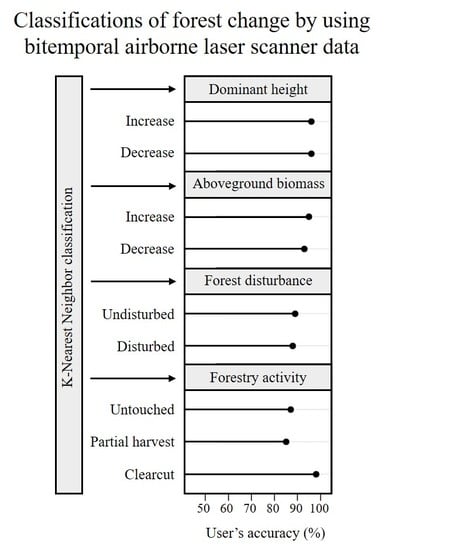
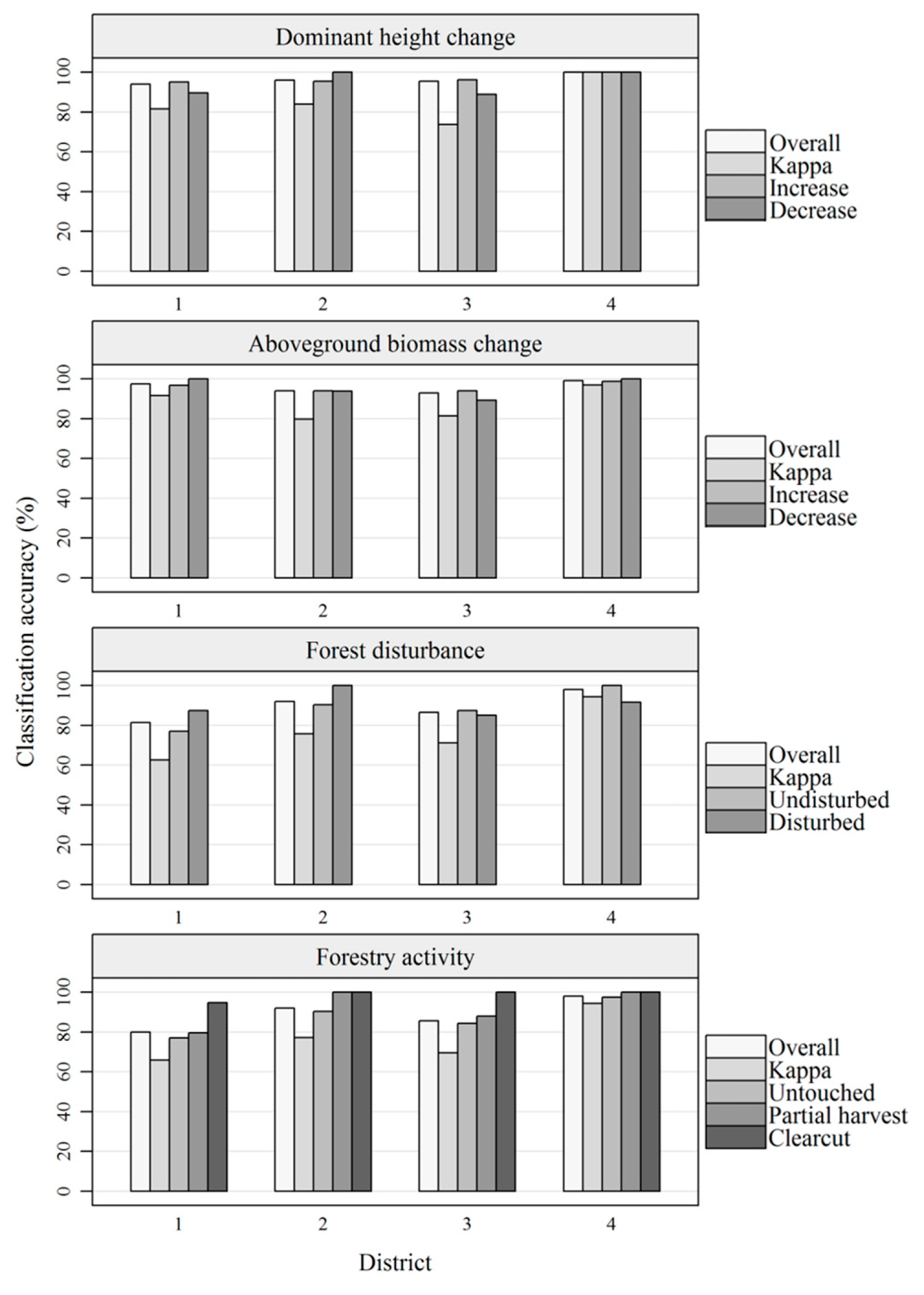
Overall accuracies obtained for Hdom and AGB change classifications were similar across the four districts, however, highest for district 4 (Figure 3). For forest disturbance and forestry activity classifications, overall accuracies differed substantially across districts, also being highest for district 4. For the classification of forestry activity, the lowest accuracies were obtained for class A, i.e., untouched forest. Classifications of clearcut plots were 100% accurate in districts 2, 3, and 4; however, in district 1, one clearcut plot was misclassified as partially harvested.

Regarding the accuracies calculated from aggregated confusion matrices for the four districts, user’s accuracies tended to be similar across classes (

Table 5. Aggregated confusion matrix of dominant height change classifications for the four districts.

Predicted	Reference		Total	User’s Accuracy (%)
	Increase	Decrease
Increase	462	20	480	96
Decrease	3	73	76	96
Total	465	93	558
Kappa			0.83
Overall accuracy (%)			96

,

Table 6. Aggregated confusion matrix of aboveground biomass change classifications for the four districts.

Predicted	Reference		Total	User’s Accuracy (%)
	Increase	Decrease
Increase	429	22	451	95
Decrease	7	100	107	93
Total	436	122	558
Kappa			0.83
Overall accuracy (%)			95

,

Table 7. Aggregated confusion matrix of forest disturbance classifications for the four districts.

Predicted	Reference		Total	User’s Accuracy (%)
	Undisturbed	Disturbed
Undisturbed	350	44	394	89
Disturbed	19	145	164	88
Total	369	189	558
Kappa			0.74
Overall accuracy (%)			89

, and

Table 8. Aggregated confusion matrix of forestry activity classifications for the four districts.

Predicted	Reference			Total	User’s Accuracy (%)
	Untouched	Partial Harvest	Clearcut
Untouched	355	50	1	406	87
Partial harvest	14	83	1	98	85
Clearcut	0	1	53	54	98
Total	369	134	55	558
Kappa				0.74
Overall accuracy (%)				88

). However, the forestry activity class “clearcut” stood out with particularly high accuracy. The misclassifications of forestry activity were mainly caused by confusion between “untouched” and “partial harvest” classes.

4. Discussion

Our results show that bitemporal data acquired as part of repeated ALS-based forest inventories are highly suitable for plot-level forest change classification. Forest planning systems in Norway, as well as many other countries, rely on information acquired in local forest inventories, and monitoring forest change at local levels is fundamental for sustainable forest management. The kNN method proved to be a practical and effective way of classifying the different changes in forest structure and yielded high accuracies. This is encouraging because the availability of bitemporal datasets will increase as local ALS-based forest inventories are repeated. The area-based approach is the most common method for predicting forest attributes from ALS data, and the methods proposed here can thus easily be applied in repeated ALS-based inventories.

Changes in ALS data proved to be good indicators of various types of forest change. This was expected because the ALS metrics that we computed characterize the height and density of the canopy at t₁ and t₂, and changes therein. Some sources of uncertainty must, however, be anticipated at the separate points in time, such as measurement errors, co-location errors between field and ALS data, and allometric errors. Moreover, additional sources of uncertainty arise when employing bitemporal field and ALS data for change detection, such as co-location errors between t₁ and t₂ plot center coordinates which may have influenced classifications negatively. Although state of the art positioning systems were used during both inventory cycles, the locations of plot centers differed in cases where the center mark was not found at t₂. In those cases, mean distances between post-processed t₁ and t₂ center coordinates were minimal, i.e., 1.1, 0.5, 0.3, and 0.5 m for districts 1–4, respectively. Nevertheless, even small positional errors will likely result in trees being in- or excluded in the plot data from the respective inventory cycles, and will therefore have caused inconsistencies in the classification of field data into change classes. Furthermore, changes in boundary effects may have added to this uncertainty. Different portions of the canopy returns within plots will have belonged to trees of which the stem was located outside of the plot and vice versa, and such boundary effects will not have been constant for t₁ and t₂.

In spite of the abovementioned challenges, classifications of Hdom change yielded high overall accuracies, and even 100% accuracy for both Hdom change classes in district 4. Local differences in species compositions may partly explain the obtained accuracies being particularly high in district 4, as it is spruce-dominated and noticeably homogenous compared to other districts. Resultantly, the forest canopy structure can also be expected to be relatively homogeneous. Crown shapes of spruce and pine trees differ, which is known to influence the values of ALS height and density metrics [64]. Tree crowns of spruce trees are narrower, longer, and more cone-shaped than those of pine and deciduous trees, which will generally skew ALS height and density metrics toward lower values [51]. Therefore, stratification according to species and forest productivity is common practice in Norwegian forest inventories, and the two are strongly linked because spruce typically grows on high productivity sites and pine on poorer sites. Stratification can potentially improve the accuracy of ALS-based predictions [65], and stratification by dominant tree species may have improved classification accuracies in other districts. However, we chose to pool all plots together to maintain large reference sets covering a broad and continuous range of forest change examples, and thus to limit the number of classifications for target units of which ALS metrics fall outside the range of the reference set.

We obtained high overall accuracies for classifications of AGB change. A kappa value of 0.87 across districts indicated an “almost perfect” agreement between observed and predicted classes according to Landis and Koch [66]. This result was expected, as ALS is a proven tool for AGB estimation [67,68,69,70], and bitemporal ALS data can therefore be expected to be well suited for classification of AGB change. The classification for district 4 yielded the highest overall accuracy, likely due to the homogeneity of the species composition. Findings presented by Næsset and Gobakken [17] also support this, as they found that tree species had a strong effect on relationships between AGB and ALS data. The classifier for district 1 performed nearly as well, with an overall accuracy of 97%, which may be explained by the relatively large portion of plots that had been harvested during the observation period (Table 1), in which case changes in AGB are particularly distinct.

Using decreases in Hdom, AGB, and N as proxies for forest disturbances, our results demonstrated that such changes in forest structure can be detected reliably from bitemporal ALS data. The use of remotely sensed data for forest disturbance detection has been studied extensively, although most studies have focused on the use of spectral-temporal information derived from time series of satellite imagery. The overall accuracy of 89% across districts is in line with accuracies reported in many of those studies. Using the Landsat archive, high overall accuracies have been reported for stand-replacing forest disturbance classifications, for example 93% [71], 88% [72], 90% [73], and 88% [74]. However, studies that included non-stand replacing disturbances in the classification reported lower overall accuracies; 75% [73] and 80% [75], likely because subtle forest changes do not tend to display a clear spectral change that can be linked to a change in land cover class [76,77]. Thus far, however, no study has investigated the use of bitemporal ALS data for the classification of structural forest changes that indicate disturbance at plot-level, and our results demonstrate that also minor decreases in Hdom, ABG, and N can be detected reliably using such data.

It must be noted, however, that defining forest disturbance on the basis of forest inventory data is not trivial. Essentially, a forest disturbance can be any event that leads to a substantial reduction in structural forest attributes and can be caused by a range of anthropogenic or naturogenic factors. Different types and intensities of disturbances can occur, and particularly minor disturbances may be challenging to detect from bitemporal ALS data with time intervals >10 years. For example, selective harvest, disease, or insect damage may have disturbed even those plots for which field-based criteria indicated they were undisturbed. A shorter observation period may ensure that such minor disturbances are detected; Yu et al. [47] showed that single harvested trees can be detected reliably from bitemporal ALS data with a temporal resolution of two years. In this study, however, we used bitemporal data with intervals of 11–15 years, which are common temporal resolutions in repeated ALS-based forest management inventories, meaning that minor disturbances may not always be captured.

We obtained high overall accuracies for the classification of forestry activities, which revealed that disturbed plots can reliably be further classified into “partial harvest” and “clearcut”. Clearcut plots were easily identified, which can be expected because a substantial loss of AGB should be easy to detect from changes in ALS metrics that reflect canopy height and density. Overall accuracies ranged from 80% to 98% across districts, with a mean of 88%. These results are similar to findings reported by Næsset et al. [34], who obtained an overall accuracy of 94% for classification of the same activity classes from bitemporal ALS data. In the mentioned study, identical field-based criteria were used to define the activity classes, a temporal resolution similar to those used in this study was used; 11 years, however, the study area was substantially smaller. Comparable to their results, discriminating between untouched and partially harvested plots proved difficult in comparison to discriminating between partially harvested and clearcut plots. This may be expected as certain subtle changes in Hdom, AGB, and especially N may not be detectable from bitemporal ALS data at temporal resolutions >10 years. ALS data are poorly suited to characterize N in comparison to other forest attributes commonly estimated in forest inventories [53], and the detection of changes in N can therefore be expected to be more challenging than changes in Hdom and AGB.

5. Conclusions

Our results show that bitemporal data acquired as part of repeated ALS-based forest inventories can be used to classify various changes in forest structure reliably. At the spatial resolution of plots used in this study and at temporal resolutions of 11–15 years, changes in Hdom and AGB can be expected to be classified with overall accuracies >90%. Forest disturbances and forestry activities were classified with overall accuracies of 89 and 88%, respectively. These results are encouraging because the availability of bitemporal field and ALS data can be expected to increase as local forest inventories are repeated, enabling the operational application of the methods proposed here.

References

- Foley, J.A.; DeFries, R.; Asner, G.P.; Barford, C.; Bonan, G.; Carpenter, S.R.; Gibbs, H.K. Global consequences of land use. Science 2005, 309, 570–574. [Google Scholar] [CrossRef] [PubMed]
- Meyer, W.B.; Turner, B.L. Human Population Growth and Global Land-Use/Cover Change. Annu. Rev. Ecol. Syst. 1992, 23, 39–61. [Google Scholar] [CrossRef]
- Yang, S.; Zhao, W.; Liu, Y.; Wang, S.; Wang, J.; Zhai, R. Influence of land use change on the ecosystem service trade-offs in the ecological restoration area: Dynamics and scenarios in the Yanhe watershed, China. Sci. Total Environ. 2018, 644, 556–566. [Google Scholar] [CrossRef] [PubMed]
- Chaplin-Kramer, R.; Sharp, R.P.; Mandle, L.; Sim, S.; Johnson, J.; Butnar, I.; Mueller, C. Spatial patterns of agricultural expansion determine impacts on biodiversity and carbon storage. Proc. Natl. Acad. Sci. USA 2015, 112, 7402–7407. [Google Scholar] [CrossRef] [PubMed] [Green Version]
- Mazor, T.; Doropoulos, C.; Schwarzmueller, F.; Gladish, D.W.; Kumaran, N.; Merkel, K.; Gagic, V. Global mismatch of policy and research on drivers of biodiversity loss. Nat. Ecol. Evol. 2018, 2, 1071. [Google Scholar] [CrossRef] [PubMed]
- Tomppo, E.; Gschwantner, T.; Lawrence, M.; McRoberts, R.E.; Gabler, K.; Schadauer, K.; Cienciala, E. National Forest Inventories. Pathways for Common Reporting; European Science Foundation: Strasbourg, France, 2010; pp. 541–553. [Google Scholar]
- Vidal, C.; Alberdi, I.; Redmond, J.; Vestman, M.; Lanz, A.; Schadauer, K. The role of European National Forest Inventories for international forestry reporting. Ann. For. Sci. 2016, 73, 793–806. [Google Scholar] [CrossRef] [Green Version]
- Breidenbach, J.; Astrup, R. Small area estimation of forest attributes in the Norwegian National Forest Inventory. Eur. J. For. Res. 2012, 131, 1255–1267. [Google Scholar] [CrossRef]
- Houborg, R.; Fisher, J.B.; Skidmore, A.K. Advances in Remote Sensing of Vegetation Function and Traits; Elsevier: Amsterdam, The Netherlands, 2015. [Google Scholar]
- White, J.C.; Coops, N.C.; Wulder, M.A.; Vastaranta, M.; Hilker, T.; Tompalski, P. Remote sensing technologies for enhancing forest inventories: A review. Can. J. Remote Sens. 2016, 42, 619–641. [Google Scholar] [CrossRef]
- Hansen, M.C.; Potapov, P.V.; Moore, R.; Hancher, M.; Turubanova, S.A.; Tyukavina, A.; Townshend, J.R.G. High-Resolution Global Maps of 21st-Century Forest Cover Change. Science 2013, 342, 850–853. [Google Scholar] [CrossRef] [Green Version]
- Sexton, J.O.; Song, X.P.; Feng, M.; Noojipady, P.; Anand, A.; Huang, C.; DiMiceli, C. Global, 30-m resolution continuous fields of tree cover: Landsat-based rescaling of MODIS vegetation continuous fields with lidar-based estimates of error. Int. J. Digit. Earth 2013, 6, 427–448. [Google Scholar] [CrossRef] [Green Version]
- Duncanson, L.; Armston, J.; Disney, M.; Avitabile, V.; Barbier, N.; Calders, K.; Crowther, T. The importance of consistent global forest aboveground biomass product validation. Surv. Geophys. 2019, 40, 979–999. [Google Scholar] [CrossRef] [PubMed]
- Herold, M.; Carter, S.; Avitabile, V.; Espejo, A.B.; Jonckheere, I.; Lucas, R.; McRoberts, R.; Næsset, E.; Nightingale, J.; Petersen, R.; et al. The Role and Need for Space-Based Forest Biomass-Related Measurements in Environmental Management and Policy. Surv. Geophys. 2019, 40, 757–778. [Google Scholar] [CrossRef] [Green Version]
- Vauhkonen, J.; Maltamo, M.; McRoberts, R.; Næsset, E. Introduction to Forestry Applications of Airborne Laser Scanning. In Forestry Applications of Airborne Laser Scanning; Maltamo, M., Næsset, E., Vauhkonen, J., Eds.; Springer: Dordrecht, The Netherlands, 2014; Volume 27, pp. 1–16. [Google Scholar]
- Maltamo, M.; Næsset, E.; Vauhkonen, J. Forestry Applications of Airborne Laser Scanning. Concepts and Case Studies; Managing Forest Ecosystems; Springer: Dordrecht, The Netherlands, 2014; Volume 27, p. 460. [Google Scholar]
- Næsset, E.; Gobakken, T. Estimation of above-and below-ground biomass across regions of the boreal forest zone using airborne laser. Remote Sens. Environ. 2008, 112, 3079–3090. [Google Scholar] [CrossRef]
- Næsset, E. Predicting forest stand characteristics with airborne scanning laser using a practical two-stage procedure and field data. Remote Sens. Environ. 2002, 80, 88–99. [Google Scholar] [CrossRef]
- White, J.C.; Wulder, M.A.; Varhola, A.; Vastaranta, M.; Coops, N.C.; Cook, B.D.; Woods, M. A best practices guide for generating forest inventory attributes from airborne laser scanning data using an area-based approach. For. Chron. 2013, 89, 722–723. [Google Scholar] [CrossRef] [Green Version]
- Niemi, M.; Vastaranta, M.; Peuhkurinen, J.; Holopainen, M. Forest inventory attribute prediction using airborne laser scanning in low-productive forestry-drained boreal peatlands. Silva Fenn. 2015. [Google Scholar] [CrossRef]
- Ståhl, G.; Holm, S.; Gregoire, T.G.; Gobakken, T.; Næsset, E.; Nelson, R. Model-based inference for biomass estimation in a LiDAR sample survey in Hedmark County, Norway. Can. J. For. Res. 2010, 41, 96–107. [Google Scholar] [CrossRef]
- Chirici, G.; Mura, M.; McInerney, D.; Py, N.; Tomppo, E.O.; Waser, L.T.; McRoberts, R.E. A meta-analysis and review of the literature on the k-Nearest Neighbors technique for forestry applications that use remotely sensed data. Remote Sens. Environ. 2016, 176, 282–294. [Google Scholar] [CrossRef]
- Xu, M.; Watanachaturaporn, P.; Varshney, P.K.; Arora, M.K. Decision tree regression for soft classification of remote sensing data. Remote Sens. Environ. 2005, 97, 322–336. [Google Scholar] [CrossRef]
- Niska, H.; Skon, J.P.; Packalen, P.; Tokola, T.; Maltamo, M.; Kolehmainen, M. Neural networks for the prediction of species-specific plot volumes using airborne laser scanning and aerial photographs. IEEE Trans. Geosci. Remote Sens. 2009, 48, 1076–1085. [Google Scholar] [CrossRef]
- McRoberts, R.E. Estimating forest attribute parameters for small areas using nearest neighbors techniques. For. Ecol. Manag. 2012, 272, 3–12. [Google Scholar] [CrossRef]
- Næsset, E.; Gobakken, T. Estimating forest growth using canopy metrics derived from airborne laser scanner data. Remote Sens. Environ. 2005, 96, 453–465. [Google Scholar] [CrossRef]
- Yu, X.; Hyyppä, J.; Kukko, A.; Maltamo, M.; Kaartinen, H. Change detection techniques for canopy height growth measurements using airborne laser scanner data. Photogramm. Eng. Remote Sens. 2006, 72, 1339–1348. [Google Scholar] [CrossRef]
- Økseter, R.; Bollandsås, O.M.; Gobakken, T.; Næsset, E. Modeling and predicting aboveground biomass change in young forest using multi-temporal airborne laser scanner data. Scand. J. For. Res. 2015, 30, 458–469. [Google Scholar] [CrossRef]
- Skowronski, N.S.; Clark, K.L.; Gallagher, M.; Birdsey, R.A.; Hom, J.L. Airborne laser scanner-assisted estimation of aboveground biomass change in a temperate oak–pine forest. Remote Sens. Environ. 2014, 151, 166–174. [Google Scholar] [CrossRef]
- Zhao, K.; Suarez, J.C.; Garcia, M.; Hu, T.; Wang, C.; Londo, A. Utility of multitemporal lidar for forest and carbon monitoring: Tree growth, biomass dynamics, and carbon flux. Remote Sens. Environ. 2018, 204, 883–897. [Google Scholar] [CrossRef]
- Bollandsås, O.M.; Ørka, H.O.; Dalponte, M.; Gobakken, T.; Næsset, E. Modelling Site Index in Forest Stands Using Airborne Hyperspectral Imagery and Bi-Temporal Laser Scanner Data. Remote Sens. 2019, 11, 1020. [Google Scholar] [CrossRef]
- Noordermeer, L.; Bollandsås, O.M.; Gobakken, T.; Næsset, E. Direct and indirect site index determination for Norway spruce and Scots pine using bitemporal airborne laser scanner data. For. Ecol. Manag. 2018, 428, 104–114. [Google Scholar] [CrossRef]
- Solberg, S.; Kvaalen, H.; Puliti, S. Age-independent site index mapping with repeated single-tree airborne laser scanning. Scand. J. For. Res. 2019, 1–31. [Google Scholar] [CrossRef]
- Næsset, E.; Bollandsås, O.M.; Gobakken, T.; Gregoire, T.G.; Ståhl, G. Model-assisted estimation of change in forest biomass over an 11 year period in a sample survey supported by airborne LiDAR: A case study with post-stratification to provide “activity data”. Remote Sens. Environ. 2013, 128, 299–314. [Google Scholar] [CrossRef]
- Daskalova, G.N.; Myers-Smith, I.H.; Bjorkman, A.D.; Blowes, S.A.; Supp, S.R.; Magurran, A.; Dornelas, M. Forest loss as a catalyst of population and biodiversity change. bioRxiv 2018, 473645. [Google Scholar] [CrossRef]
- Franklin, J.F.; Spies, T.A.; Van Pelt, R.; Carey, A.B.; Thornburgh, D.A.; Berg, D.R.; Shaw, D.C. Disturbances and structural development of natural forest ecosystems with silvicultural implications, using Douglas-fir forests as an example. For. Ecol. Manag. 2002, 155, 399–423. [Google Scholar] [CrossRef]
- Seidl, R.; Thom, D.; Kautz, M.; Martin-Benito, D.; Peltoniemi, M.; Vacchiano, G.; Honkaniemi, J. Forest disturbances under climate change. Nat. Clim. Chang. 2017, 7, 395. [Google Scholar] [CrossRef]
- Thom, D.; Seidl, R. Natural disturbance impacts on ecosystem services and biodiversity in temperate and boreal forests. Biol. Rev. 2016, 91, 760–781. [Google Scholar] [CrossRef]
- Raymond, C.L.; Healey, S.; Peduzzi, A.; Patterson, P. Representative regional models of post-disturbance forest carbon accumulation: Integrating inventory data and a growth and yield model. For. Ecol. Manag. 2015, 336, 21–34. [Google Scholar] [CrossRef]
- d’Oliveira, M.V.; Reutebuch, S.E.; McGaughey, R.J.; Andersen, H.E. Estimating forest biomass and identifying low-intensity logging areas using airborne scanning lidar in Antimary State Forest, Acre State, Western Brazilian Amazon. Remote Sens. Environ. 2012, 124, 479–491. [Google Scholar] [CrossRef]
- Falkowski, M.J.; Evans, J.S.; Martinuzzi, S.; Gessler, P.E.; Hudak, A.T. Characterizing forest succession with lidar data: An evaluation for the Inland Northwest, USA. Remote Sens. Environ. 2009, 113, 946–956. [Google Scholar] [CrossRef] [Green Version]
- Valbuena, R.; Maltamo, M.; Packalen, P. Classification of multilayered forest development classes from low-density national airborne lidar datasets. For. Int. J. For. Res. 2016, 89, 392–401. [Google Scholar] [CrossRef] [Green Version]
- Van Ewijk, K.Y.; Treitz, P.M.; Scott, N.A. Characterizing forest succession in Central Ontario using LiDAR-derived indices. Photogramm. Eng. Remote Sens. 2011, 77, 261–269. [Google Scholar] [CrossRef]
- Eysn, L.; Hollaus, M.; Schadauer, K.; Pfeifer, N. Forest delineation based on airborne LIDAR data. Remote Sens. 2012, 4, 762–783. [Google Scholar] [CrossRef]
- Olofsson, K.; Holmgren, J. Forest stand delineation from lidar point-clouds using local maxima of the crown height model and region merging of the corresponding Voronoi cells. Remote Sens. Lett. 2014, 5, 268–276. [Google Scholar] [CrossRef]
- Sačkov, I.; Kardoš, M. Forest delineation based on LiDAR data and vertical accuracy of the terrain model in forest and non-forest area. Ann. For. Res. 2014, 57, 119–136. [Google Scholar] [CrossRef]
- Yu, X.; Hyyppä, J.; Kaartinen, H.; Maltamo, M. Automatic detection of harvested trees and determination of forest growth using airborne laser scanning. Remote Sens. Environ. 2004, 90, 451–462. [Google Scholar] [CrossRef]
- Nyström, M.; Holmgren, J.; Olsson, H. Change detection of mountain birch using multi-temporal ALS point clouds. Remote Sens. Lett. 2013, 4, 190–199. [Google Scholar] [CrossRef]
- Solberg, S. Mapping gap fraction, LAI and defoliation using various ALS penetration variables. Int. J. Remote Sens. 2010, 31, 1227–1244. [Google Scholar] [CrossRef]
- St-Onge, B.; Vepakomma, U. Assessing forest gap dynamics and growth using multi-temporal laser-scanner data. Int. Arch. Photogramm. Remote Sens. Spat. Inf. Sci. 2004, 36, 173–178. [Google Scholar]
- Næsset, E. Practical large-scale forest stand inventory using a small-footprint airborne scanning laser. Scand. J. For. Res. 2004, 19, 164–179. [Google Scholar] [CrossRef]
- Næsset, E. Accuracy of forest inventory using airborne laser scanning: Evaluating the first Nordic full-scale operational project. Scand. J. For. Res. 2004, 19, 554–557. [Google Scholar] [CrossRef]
- Næsset, E. Airborne laser scanning as a method in operational forest inventory: Status of accuracy assessments accomplished in Scandinavia. Scand. J. For. Res. 2007, 22, 433–442. [Google Scholar] [CrossRef]
- Gobakken, T.; Næsset, E. Assessing effects of laser point density, ground sampling intensity, and field sample plot size on biophysical stand properties derived from airborne laser scanner data. Can. J. For. Res. 2008, 38, 1095–1109. [Google Scholar] [CrossRef]
- Anonymous. Handbok for Planlegging I Skogbruket; Landbruksforlaget: Oslo, Norway, 1987; Available online: https://www.nb.no/nbsok/nb/c55d16a811d846645632638cb893d749 (accessed on 23 August 2019).
- Topcon Positioning Systems. MAGNET Tools 1.0.; Topcon Positioning Systems Inc.: Livermore, CA, USA, 2012. [Google Scholar]
- Ørka, H.O.; Bollandsås, O.M.; Hansen, E.H.; Næsset, E.; Gobakken, T. Effects of terrain slope and aspect on the error of ALS-based predictions of forest attributes. For. Int. J. For. Res. 2018, 91, 225–237. [Google Scholar] [CrossRef] [Green Version]
- García, O. Estimating top height with variable plot sizes. Can. J. For. Res. 1998, 28, 1509–1517. [Google Scholar] [CrossRef]
- Marklund, L.G. Biomass Functions for Pine, Spruce and Birch in Sweden; Rapport-Sveriges Lantbruksuniversitet, Institutionen foer Skogstaxering: Uppsala, Sweden, 1988. [Google Scholar]
- Cover, T.M.; Hart, P. Nearest neighbor pattern classification. IEEE Trans. Inf. Theory 1967, 13, 21–27. [Google Scholar] [CrossRef]
- Maltamo, M.; Malinen, J.; Packalén, P.; Suvanto, A.; Kangas, J. Nonparametric estimation of stem volume using airborne laser scanning, aerial photography, and stand-register data. Can. J. For. Res. 2006, 36, 426–436. [Google Scholar] [CrossRef]
- Cohen, J. A coefficient of agreement for nominal scales. Educ. Psychol. Meas. 1960, 20, 37–46. [Google Scholar] [CrossRef]
- Hand, D.J. Assessing the Performance of Classification Methods. Int. Stat. Rev. 2012, 80, 400–414. [Google Scholar] [CrossRef]
- Nelson, R. Modeling forest canopy heights: The effects of canopy shape. Remote Sens. Environ. 1997, 60, 327–334. [Google Scholar] [CrossRef]
- Næsset, E. Area-based inventory in Norway–from innovation to an operational reality. In Forestry Applications of Airborne Laser Scanning; Springer: Berlin/Heidelberg, Germany, 2014; pp. 215–240. [Google Scholar]
- Landis, J.R.; Koch, G.G. The measurement of observer agreement for categorical data. Biometrics 1977, 33, 159–174. [Google Scholar] [CrossRef]
- Aardt, J.A.V.; Wynne, R.H.; Oderwald, R.G. Forest volume and biomass estimation using small-footprint lidar-distributional parameters on a per-segment basis. For. Sci. 2006, 52, 636–649. [Google Scholar]
- Bortolot, Z.J.; Wynne, R.H. Estimating forest biomass using small footprint LiDAR data: An individual tree-based approach that incorporates training data. ISPRS J. Photogramm. Remote Sens. 2005, 59, 342–360. [Google Scholar] [CrossRef]
- Gregoire, T.G.; Ståhl, G.; Næsset, E.; Gobakken, T.; Nelson, R.; Holm, S. Model-assisted estimation of biomass in a LiDAR sample survey in Hedmark County, Norway. Can. J. For. Res. 2010, 41, 83–95. [Google Scholar] [CrossRef]
- Jochem, A.; Hollaus, M.; Rutzinger, M.; Höfle, B. Estimation of aboveground biomass in alpine forests: A semi-empirical approach considering canopy transparency derived from airborne LiDAR data. Sensors 2011, 11, 278–295. [Google Scholar] [CrossRef]
- Cohen, W.B.; Fiorella, M.; Gray, J.; Helmer, E.; Anderson, K. An efficient and accurate method for mapping forest clearcuts in the Pacific Northwest using Landsat imagery. Photogramm. Eng. Remote Sens. 1998, 64, 293–299. [Google Scholar]
- Cohen, W.B.; Spies, T.A.; Alig, R.J.; Oetter, D.R.; Maiersperger, T.K.; Fiorella, M. Characterizing 23 years (1972–95) of stand replacement disturbance in western Oregon forests with Landsat imagery. Ecosystems 2002, 5, 122–137. [Google Scholar] [CrossRef]
- Ahmed, O.S.; Wulder, M.A.; White, J.C.; Hermosilla, T.; Coops, N.C.; Franklin, S.E. Classification of annual non-stand replacing boreal forest change in Canada using Landsat time series: A case study in northern Ontario. Remote Sens. Lett. 2017, 8, 29–37. [Google Scholar] [CrossRef]
- Huo, L.Z.; Boschetti, L.; Sparks, A.M. Object-Based Classification of Forest Disturbance Types in the Conterminous United States. Remote Sens. 2019, 11, 477. [Google Scholar] [CrossRef]
- Huang, C.; Goward, S.N.; Masek, J.G.; Thomas, N.; Zhu, Z.; Vogelmann, J.E. An automated approach for reconstructing recent forest disturbance history using dense Landsat time series stacks. Remote Sens. Environ. 2010, 114, 183–198. [Google Scholar] [CrossRef]
- Franklin, S.E.; Ahmed, O.S.; Wulder, M.A.; White, J.C.; Hermosilla, T.; Coops, N.C. Large area mapping of annual land cover dynamics using multitemporal change detection and classification of Landsat time series data. Can. J. Remote Sens. 2015, 41, 293–314. [Google Scholar] [CrossRef]
- Hermosilla, T.; Wulder, M.A.; White, J.C.; Coops, N.C.; Hobart, G.W. Regional detection, characterization, and attribution of annual forest change from 1984 to 2012 using Landsat-derived time-series metrics. Remote Sens. Environ. 2015, 170, 121–132. [Google Scholar] [CrossRef]
Figure 1.
Map of southeastern Norway showing the location of the four districts. White lines represent county borders.
Figure 2.
Box plots showing the distribution of computed field plot data.
Figure 3.
Classification accuracies.