1. Introduction
Latent and sensible heat fluxes (LHF and SHF, respectively) over the Earth’s oceans, produced by turbulent flow within the planetary boundary layer, can have a significant effect on the genesis and evolution of various weather and climate systems. LHF and SHF are primarily driven by surface wind speeds and differences in temperature and specific humidity between the lowest levels of the atmosphere (~10 meters above the surface) and the sea surface [
1]. Influxes of moisture and thermal energy can decrease the static stability within the boundary layer, decreasing the height of the lifted condensation level, potentially leading to the development of dry and moist convection [
2,
3]. The energy transported between the ocean surface and lower atmosphere influences the development of various weather systems from the microscale up to the synoptic scale, including—isolated and organized convection [
4], tropical [
5] and extratropical cyclones [
6] and large-scale waves (e.g. Madden-Julian Oscillation (MJO)) [
7].
There are several methods that can be used to estimate surface heat fluxes but the most common method utilizes the bulk aerodynamic formulas. These formulas relate the turbulent fluxes to the observable spatial and temporal averages [
1,
8] and can be written as follows:
Here, ρa is the air density at the surface [kg m−3]; Lv is the latent heat of condensation (2.5 × 10⁶ J kg−1); and cp is specific heat at constant pressure (1004 J K−1 kg−1). CDE and CDH are, respectively, the exchange coefficients of moisture and sensible heat [unitless]; U is the magnitude of the surface wind speed [m s−1], Ts and qs are temperature [K] and specific humidity [kg kg−1], respectively, at the surface, while Ta and qa are the same but at 10 meters above the surface.
Given the impacts LHF and SHF have on weather systems at multiple scales and their rapid spatial and temporal variations, routine and widespread measurements of the surface heat fluxes are necessary. In-situ observations from flux towers and buoys have been and will continue to be the standard for LHF and SHF measurements over the world’s oceans, but they are limited spatially and temporally. While spaceborne instruments are currently unable to directly measure surface heat fluxes, they can be used to estimate the components, like temperature, humidity and wind speed, which are needed to estimate LHF and SHF through the bulk aerodynamic formulas [
9]. However, these instruments, such as microwave radiometers and scatterometers in a polar-orbit, have their own limitations. Their orbits can cause them to miss large spatial areas and/or feature infrequent sampling, especially over the lower latitudes. Additionally, their measurements are often affected by the presence of precipitation, leading to inaccurate or missing surface measurements. By utilizing its surface wind speed observations (coupled with estimates of thermodynamic variables from other sources), the Cyclone Global Navigation Satellite System (CYGNSS) can provide improved coverage of surface heat fluxes over the tropical and subtropical oceans with its high temporal and spatial sampling of ocean surface wind speed. Though CYGNSS is in a tropical orbit (35° orbit inclination), it can still observe a large swath of surface heat fluxes over the world’s tropical and subtropical oceans.
The largest latent and sensible heat fluxes are often observed in the extratropical regions during the respective winter seasons of both hemispheres [
10]. This is because surface wind speeds and differences in temperature and humidity are consistently at their greatest during the winter. These large heat fluxes are typically concentrated near coastlines where warm ocean waters interact with cold and dry air masses originating over continental landmasses, such as the Western Pacific and Western Atlantic Oceans, which can affect the formation of rapidly developing extratropical cyclones (ETCs) [
11,
12]. While these fluxes are at their maximum at middle and high latitudes, CYGNSS can make consistent observations up to 38° latitude in both hemispheres [
13,
14]. As Figure 2 from Yu and Weller [
10] indicates, some of the highest fluxes typically observed over the world’s oceans occur within CYGNSS’s observational range.
This paper describes the development of a Level-2 (L2) ocean Surface Heat Flux product for the entire CYGNSS mission, which utilizes its L2 wind speed retrievals, coupled with a reanalysis dataset for the thermodynamic variables (temperature and humidity). The goal of this product is to, along with in-situ and other remote sensing observations, aid the scientific community’s understanding of how latent and sensible heat fluxes impact the genesis and evolution of various weather and climate patterns across the globe by utilizing CYGNSS’s frequent sampling over the tropical and subtropical oceans.
The structure of the paper is as follows—
Section 2 introduces in detail the data that are used to estimate the surface heat fluxes for the CYGNSS mission.
Section 3 discusses the algorithm being used for the product.
Section 4 discusses initial results from the CYGNSS Surface Heat Flux Product across the globe and for two case studies.
Section 5 focuses on the comparisons with LHF and SHF estimates from buoy data, as well as how differences in the inputs (wind, temperature, humidity) correlated with differences in the fluxes.
Section 6 includes a simple uncertainty and sensitivity analysis of the CYGNSS Flux product.
Section 7 and
Section 8 contain the discussion, summary, conclusions and future uses and development of the product.
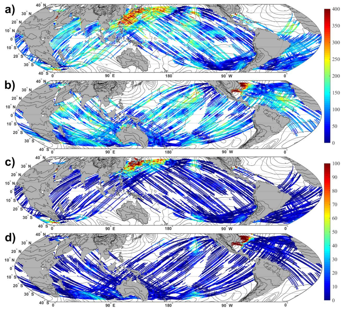
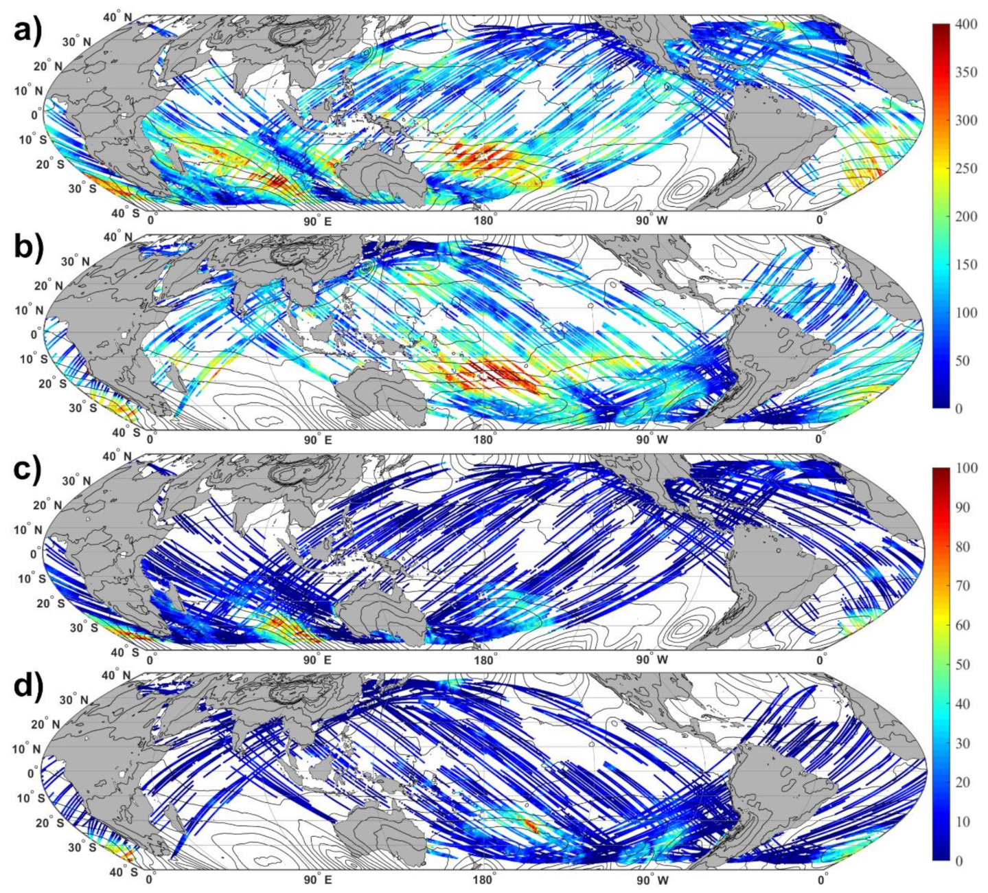
4. Results
Figure 1;
Figure 2 depict two separate full days (split into 12-hour increments) of latent and sensible heat flux estimates from CYGNSS using the FDS wind speeds. On 1 January 2018 (
Figure 1), one can see large latent and sensible heat fluxes, primarily along the Western Pacific and Western Atlantic Oceans in the Northern Hemisphere. This is expected, as large air-sea temperature and humidity differences observed during the winter seasons lead to higher heat fluxes, as well as high wind scenarios associated with possible developing winter storms. Meanwhile, the distribution of fluxes are reversed in the 1 July 2018 case (
Figure 2) as it is the winter season in the southern hemisphere, leading to higher surface heat fluxes in the South Pacific, Indian and Atlantic Oceans. Strong gradients in mean sea level pressure are co-located with some regions of high heat flux, indicating the correlation between high wind speeds and large positive surface heat fluxes.
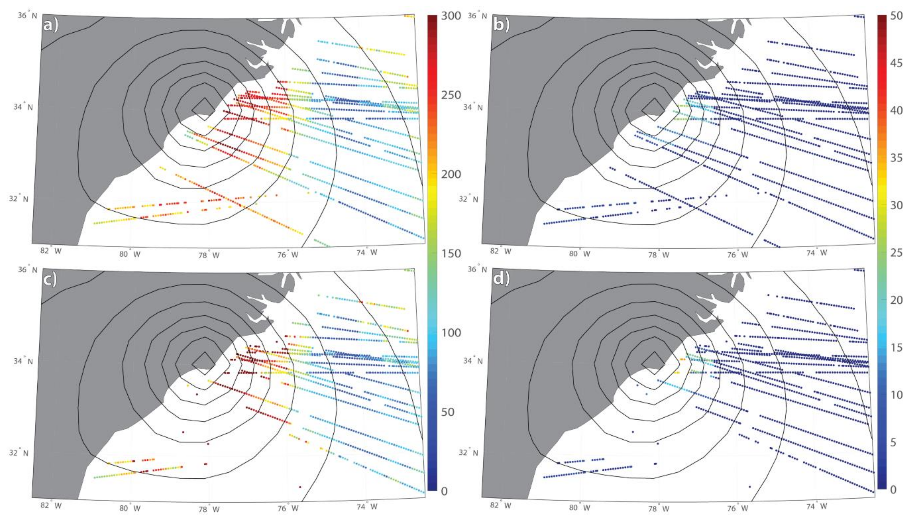
In September 2018, Hurricane Florence made landfall along the North Carolina shore but after landfall, its center of circulation moved to the southwest along the coast, causing heavy rainfall and major coastal flooding in the area. As post-landfall Florence travelled along the North Carolina coast, CYGNSS was able to observe the cyclone and estimate its associated surface heat fluxes. Around 18:00 UTC on 14 September, LHF observations from both FDS and YSLF products exceeded 300 W/m
2 (
Figure 3a,b), though SHF observations hardly exceeded 30 W/m
2 (
Figure 3c,d). While there were latent heat flux values in and around Florence up to 300 W/m
2 prior to landfall, regions containing high fluxes were not as widespread as high-flux regions observed after landfall. While the high wind speeds observed in Florence certainly contributed to the high latent heat fluxes, the large air-sea differences after landfall had an influence as well. In its western half, Florence was able to pull in drier air from the continent, which then interacted with the warm Gulf Stream ocean surface on its southern and eastern halves, contributing to the high latent heat fluxes observed in concert with its higher wind speeds. However, SHF remained low, indicating that while the humidity differences were large, the same could not be said about the temperature differences between the surface and 10 meters. As expected, the surface fluxes that were estimated utilizing the YSLF winds were relatively high; however, one should note that there are fewer points compared to the fluxes estimated with FDS winds. This can be noticed in the southern half of the cyclone. This is expected, as YSLF wind speeds are generally higher than FDS wind speeds and are therefore more likely to surpass the 25 m/s speed limit of the COARE 3.5 algorithm and be removed through the quality flag controls.
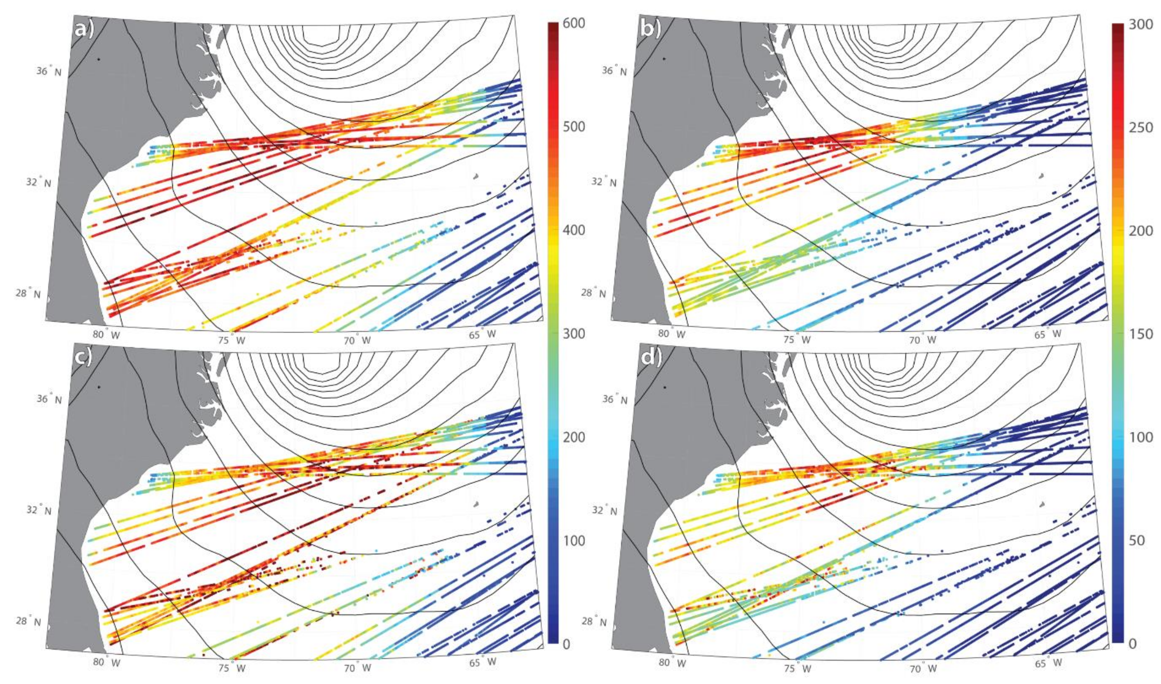
Given CYGNSS’s ability to observe low-latitude extratropical cyclones [
14], we can also obtain LHF and SHF estimates in extratropical cyclones (ETCs) that develop within CYGNSS’s range. One of the ETCs that CYGNSS observed was a rapidly developing ‘bomb cyclone’ (an ETC in which the mean sea level pressure decreases by at least 24 hPa within 24 hours [
26]) along the East Coast of the United States in January 2018 (
Figure 4). Though the ETC developed and moved poleward rapidly, CYGNSS was able to observe the equatorward side of the cyclone. The highest surface heat fluxes are typically observed on this side of a marine-based ETC, as strong winds pull cold and dry air from the continent over the warmer and moister ocean surface [
6]. As can be seen in this case study on 4 January 2018 around 15z, CYGNSS observed latent heat fluxes exceeding 600 W/m
2 and sensible heat fluxes of over 300 W/m
2 as the cyclone continued to strengthen and proceed poleward to the northeast United States. Much like the Hurricane Florence case, the LHF and SHF values estimated with YSLF winds were often higher than those estimated with FDS winds. In this case, one can clearly see that fluxes estimated from the YSLF winds are noisier than LHF and SHF estimated with FDS wind speeds. This is expected because, as mentioned in
Section 2.1, time averaging is not applied to consecutive sample points for the YSLF winds, as is done for the FDS winds, so that the highest possible horizontal spatial resolution is obtained for high wind situations.
High surface heat fluxes were observed in both the Hurricane Florence and ‘Bomb Cyclone’ ETC cases, indicating that there is a large amount of energy being transferred from the ocean surface into the lower atmosphere, which could affect how these systems evolved. While previous research has shown that high surface heat fluxes associated with these and other systems can influence their development [
4,
5,
6,
7], we cannot speculate at this time exactly how much the fluxes observed in these case studies affected their development solely based on these observations. Future modelling studies could address these specific case studies and examine how the high surface heat fluxes that were observed by CYGNSS affected their evolution.
5. Comparisons with Ground Truth Buoy Data
Direct in-situ measurements of LHF and SHF have been limited during CYGNSS’s mission, as they are often collected only during a small number of field campaigns (e.g. PISTON [
27], CAMP2Ex [
28]) and on research buoys. While comparisons with additional in-situ data may be obtained for future versions of the CYGNSS Flux Product, at this time we have used surface flux estimates derived from buoy data that are a spatial and temporal match with CYGNSS specular points. Though these buoys do not measure LHF and SHF directly, they do measure wind speeds, temperature and humidity, which can be directly inserted into the same COARE algorithm utilized for the CYGNSS Surface Heat Flux Product.
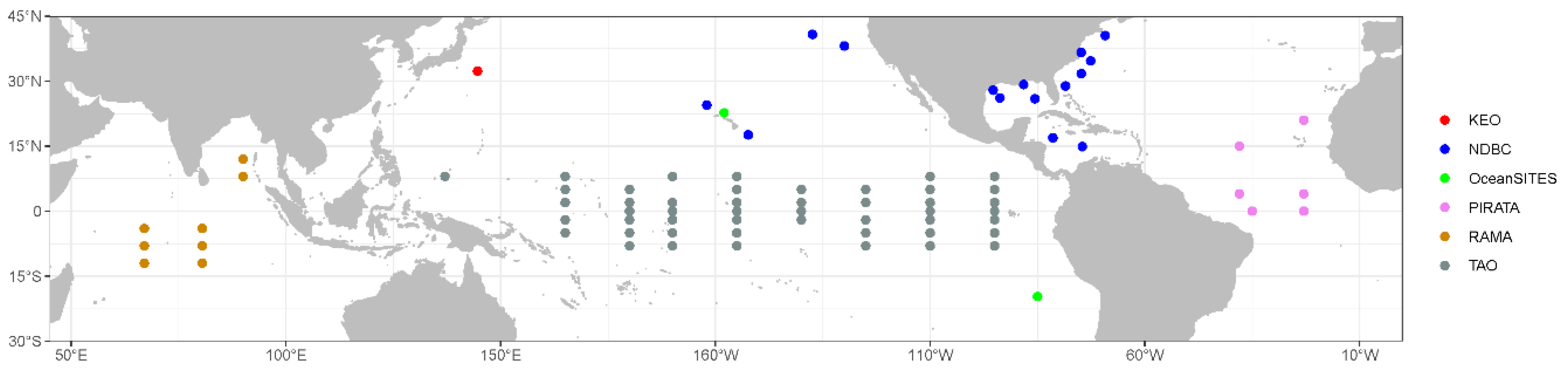
From 18 March 2017 to 29 January 2019, the CYGNSS Surface Heat Flux Product was validated against the following buoys and buoy networks (
Figure 5):
Kuroshio Extension Observatory (KEO) [
29]
National Data Buoy Center (NDBC) [
30]
Ocean Sustained Interdisciplinary Timeseries Environment observation System (OceanSITES) [
31]
Prediction and Research Moored Array in the Tropical Atlantic (PIRATA) [
32]
Research Moored Array for African-Asian-Australian Monsoon Analysis and Prediction (RAMA) [
33]
Tropical Atmosphere Ocean Array (TAO) [
34]
Data from these buoys can be accessed publicly through the National Oceanic and Atmospheric Administration (NOAA) [
35,
36,
37]. Data from the buoys were compared to the CYGNSS Fluxes following Ruf et al. [
38]. In the present analysis, CYGNSS derived flux measurements that occurred within 50 km and 0.5 hours of a buoy’s location and observation time were used, which were then collocated by an inverse-weighting scheme [
39]. Overall, 83 buoys were used for these matchups, with an aggregated sample size of 21,679 matchups for the FDS products and 20,947 matchups for the YSLF products (after applying CYGNSS Flux quality flags).
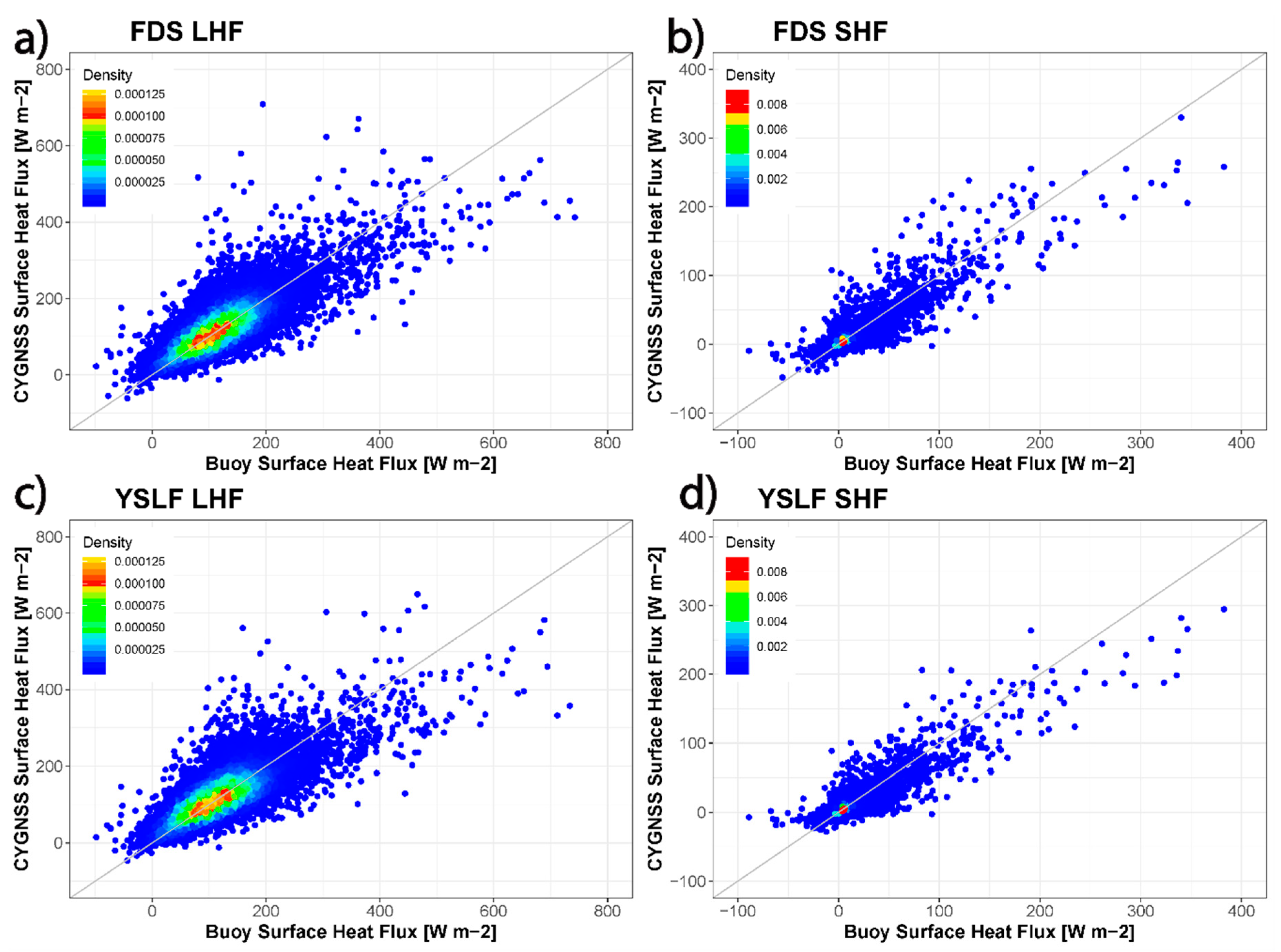
5.1. Comparisons with Buoy Data
Figure 6 shows a 2D density scatter plot of the collocated flux samples. The scatter plot demonstrates a good agreement between the CYGNSS Fluxes and the derived buoy fluxes, with a correlation around 0.8 and 0.79 for LHF with FDS and YSLF winds (respectively) and 0.85 for both SHF products (
Table 1). The highest density of matchups occur along the diagonal 1:1 line for all CYGNSS Flux products; the highest density of LHF matchups occur between 50-150 W/m
2, while the highest density of SHF matchups occur around 0 W/m
2. The CYGNSS Fluxes overall agree well with the estimates from the buoys, though there is a discrepancy at lower values (as seen in
Figure 7). However, as the surface heat fluxes increase, there is greater scatter and disagreement between CYGNSS and the buoy data. While some fluxes are overestimated, a majority of the higher CYGNSS Flux values are lower than those estimated from the buoy data. This is likely due to CYGNSS’s increased uncertainty at higher wind speeds, which have yielded lower wind speed values compared to other sources [
40]. Since wind speeds correlate with LHF and SHF based on Equations (1) and (2), if CYGNSS winds are underestimating higher wind speed values, then it should also lead to an underestimate of higher latent and sensible heat flux values. However, as will be discussed in the next section, the inputs from MERRA-2 could also be impact the disagreements between CYGNSS and buoy flux measurements.
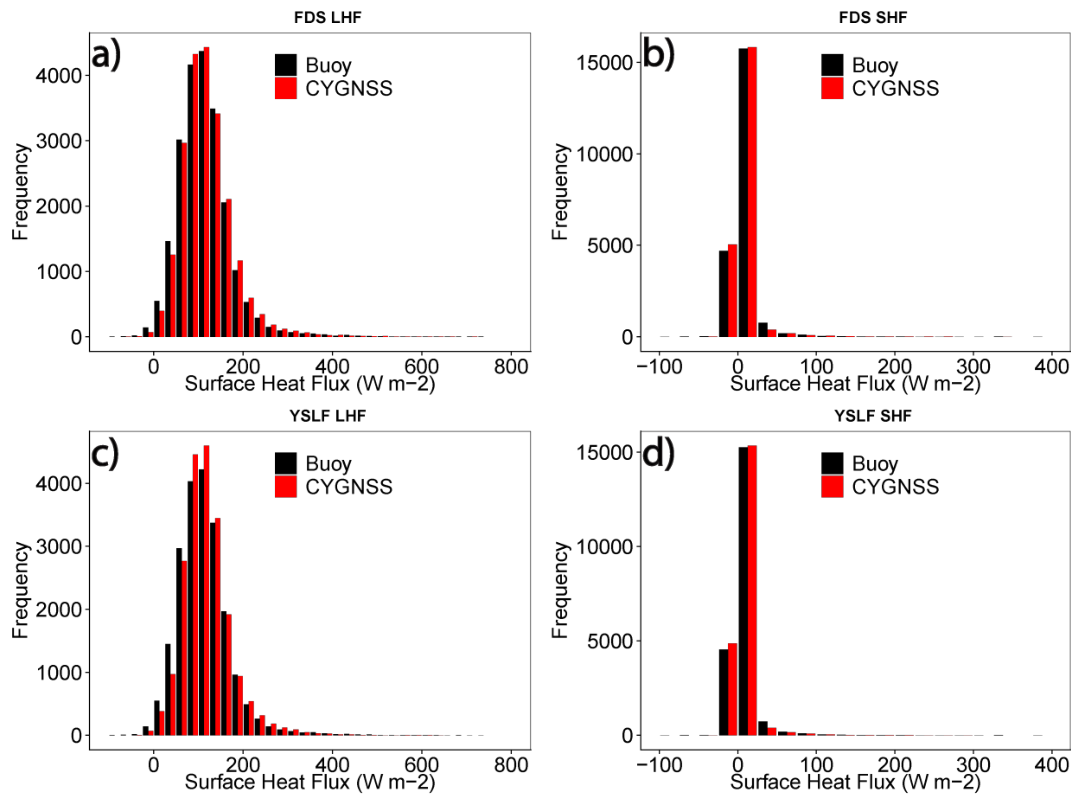
While the density plots in
Figure 6 show that a majority of the fluxes match-up well, there are still significant spread in the data at the lower flux values.
Figure 7 is a histogram of the CYGNSS Fluxes and buoy data binned in intervals of 25 W/m
2. While there are few differences in the SHF histogram, there are larger differences in the LHF plots. For LHF values between 50–200 W/m
2, we see a greater number of CYGNSS observations compared to the buoy data, while the reverse is true for values less than 50 W/m
2. These plots help us understand the additional spread around the 1:1 line observed in the density plots (
Figure 6). The differences seen in
Figure 6 and the scatter observed at higher flux values could be the result of uncertainties in the CYGNSS wind speed observations, as there have been known errors at higher wind speeds [
38,
40]. However, CYGNSS is likely not the only source of uncertainty and errors at these higher flux values. As
Section 5.2 and
Section 6 will discuss, differences in variables between MERRA-2 and the buoy data could also be contributing to these differences.
As highlighted by
Figure 7, the number of buoy and CYGNSS comparisons at higher flux values were limited in comparison to those at lower LHF and SHF values, which may have resulted in the larger scatter at higher flux values. We expect that future versions of the CYGNSS Fluxes will include comparisons and validation with flux measurements from various field campaigns, as well as a larger set of buoy comparisons, especially at the high fluxes values. In addition to validation with additional sources of data, future releases of the CYGNSS wind speeds are expected to reduce some of the errors at higher wind speeds that are currently present in the current version.
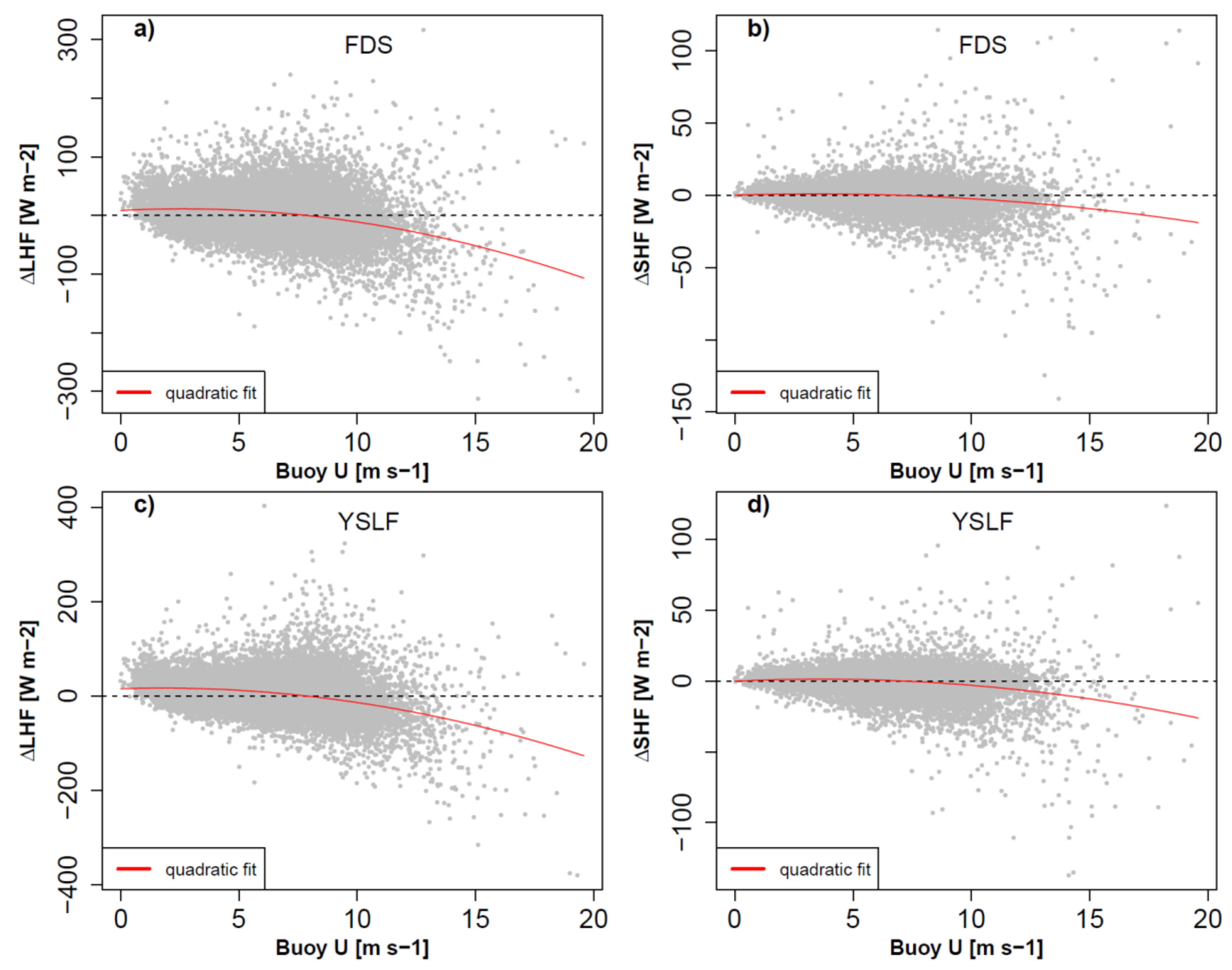
5.2. Flux Component Influence
Figure 8 shows how differences between CYGNSS Flux observations and buoy flux observations change as wind speed measurements from the buoys increases. Here, a positive difference means CYGNSS observations were greater than the buoy data and vice versa for negative differences. At lower wind speed observations, while there is a large spread between the two (similar to
Figure 6), based on the quadratic fit the differences between the CYGNSS and buoy fluxes averaged out to be near zero. Meanwhile, as wind speeds from the buoy data increases, the differences between CYGNSS and buoy flux measurements increase, with all four CYGNSS Flux products underestimating LHF and SHF with respect to the buoy data. These differences, as they correlate to wind speed, could explain why we see CYGNSS underestimate the fluxes compared to buoy data in
Figure 5. While differences in wind speed could be the main factor in these differences, as CYGNSS winds have been underestimating winds at higher wind speeds [
40], we need to look into how all inputs into the flux product could be impacting these results.
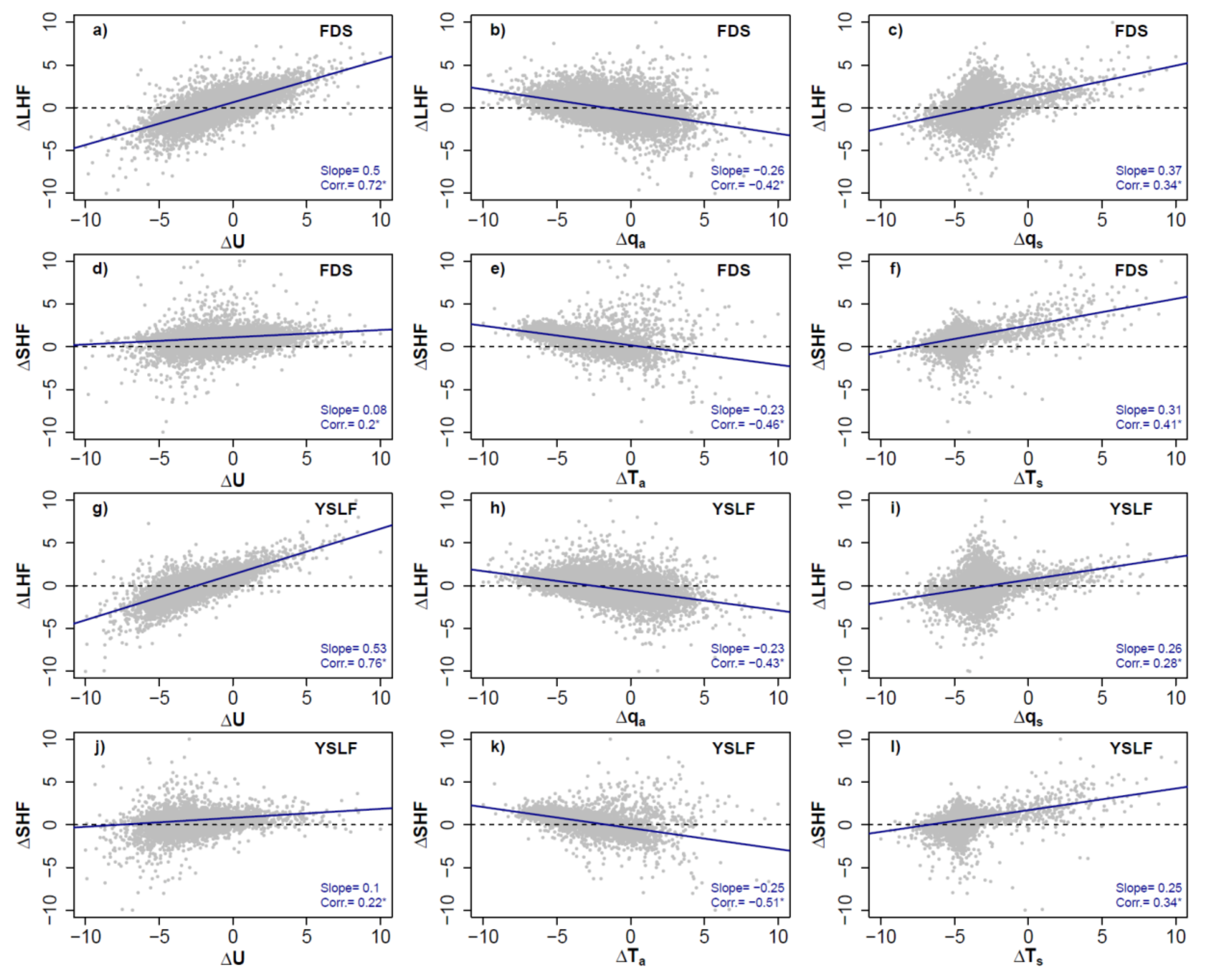
Figure 9 shows the flux residual dependency on available bulk flux component (temperature, humidity, wind speed) residual. Here, all differences are calculated as CYGNSS minus buoy and the results are normalized to the range of −10 to 10, similar to previous studies [
41]. For both latent heat flux products, differences in wind speed (Δ
U) correlate well with Δ
LHF. However, though smaller, the Δ
qa and Δ
qs have a non-negligible impact and have a correlation with Δ
LHF as well, indicating that the variables in the MERRA-2 contribute to these differences.
Meanwhile for both products of the sensible heat flux, discrepancies in wind speed between CYGNSS and buoys do not contribute much to the observed ΔSHF. However, ΔTa and ΔTs correlate more to the observed ΔSHF. This shows that while discrepancies in CYGNSS and MERRA-2 can equally contribute to observed ΔLHF, it seems that differences in MERRA-2 observations are the main contributor to observed ΔSHF.
One curious oddity in these plots are the large spread in ΔLHF and ΔSHF in the surface humidity and temperature plots, respectively, around Δqs= −5 and ΔTs= −5 (originally ΔTs= 0°C & Δqs= 0 kg/kg, respectively). While future analysis is needed to address why there is a spread in ΔLHF and ΔSHF when ΔTs and Δqs are zero, one hypothesis that could explain these differences are other factors, such as wind and 10-meter humidity/temperature could be playing a much larger role in ΔLHF and ΔSHF at these points. Additionally, it could also be due to the air-sea state or stability effect. However, future analyses are needed to fully address the oddity in this product.
6. Simple Sensitivity and Uncertainty Analysis
While the use of the COARE algorithm for the CYGNSS Flux Product has been effective in estimating LHF and SHF throughout CYGNSS’s mission, inaccuracies and uncertainties in the inputs can result in greater uncertainties in LHF and SHF. As discussed in
Section 5, variations in the inputs from CYGNSS and MERRA-2 could significantly alter the results. In order to estimate the uncertainty of the fluxes from these inputs, we first examine the impact of the known and estimated uncertainties of each input variable (wind, temperature, humidity) on the LHF and SHF results.
As an example, an uncertainty value is reported at every specular point for CYGNSS’s FDS and YSLF wind speed product. For this uncertainty analysis, at each specular point, 100 random numbers are created with a mean of zero and a standard deviation equal to the reported wind speed (FDS) uncertainty. These 100 values are then added to the FDS wind speed to produce 100 perturbed wind speed values at that specular point. The same algorithm is then applied to estimate LHF and SHF for each perturbed value of wind speed, keeping the other inputs the same. This produces 100 values each for LHF and SHF at every specular point. Then, the standard deviation of these 100 values are computed to estimate an uncertainty in LHF and SHF associated with the wind speed uncertainty.
This process is repeated for YSLF winds, surface temperature, 10-meter air temperature and relative humidity at each specular point. Unlike CYGNSS, MERRA-2 does not provide uncertainties at each grid point, so an averaged uncertainty for each variable is used across the globe (1°C for air temperature, 0.5°C for SST and 5% for relative humidity [
42,
43]). Since uncertainties for specific humidity from MERRA-2 were not available, 10-meter specific humidity was converted to relative humidity given its availability [
42]. These values are an approximate from similar studies, but future uncertainty analysis and updates for the CYGNSS Fluxes will examine how these uncertainties can vary in different conditions (e.g. precipitation, rapidly developing systems, etc.), as well as include uncertainties in specific humidity at the surface.
Once the standard deviations of LHF and SHF from each variable are computed, they are combined into one standard deviation for LHF and SHF at every specular point using the formula:
where
σLHF,Ta is the standard deviation of LHF when 10-meter air temperature is perturbed,
σLHF,Ts is the standard deviation of LHF when surface temperature is perturbed,
σLHF,RH is the standard deviation of LHF when relative humidity is perturbed and
σLHF,FDSwind is the standard deviation of LHF when FDS wind speed is perturbed (all units of W m
−2). This same method can be used to estimate
σSHF, along with
σLHF_YSLF and
σSHF_YSLF, by replacing the last input in Equation (4) with
σLHF, YSLFwind and
σSHF, YSLFwind, respectively.
Given that a single day of CYGNSS observations can yield over 2.5 million specular points throughout the entire constellation, this simple uncertainty analysis was limited to just three days (14-16 September 2017) for this study due to computational and time limits. Future analysis will include more data, as well as analyze how these uncertainties can change in different seasons, environments, basins, and so forth. Specular points were that flagged, under the criteria described in
Section 3.2, were not used for the analysis.
As shown in
Table 2, the uncertainties at each specular point over this three-day period are averaged to give the overall uncertainty for LHF and SHF, as well as the sensitivity from the individual components.
These values show how the uncertainties from CYGNSS and MERRA-2 can contribute to uncertainties observed in SHF and LHF (11 W m
2 for both SHF products, 44/51 W m
2 for the FDS/YSLF versions of LHF product, respectively). As expected, wind speed is the only input whose uncertainty impact changes between the FDS and YSLF products. While there are very small changes for temperature and humidity between the FDS and YSLF products, these are insignificant and can most likely be attributed to differences in sample points (as more YSLF points are filtered out due to higher wind speeds). Despite the large uncertainties associated with the CYGNSS winds, in most products it was not the largest source of uncertainty. Though a 1°C uncertainty was used for 10m air temperature, it led to the largest source of uncertainty in three of the four CYGNSS Flux products. As was seen in
Figure 9, differences in CYGNSS and buoy wind speeds did not contribute much to ΔSHF, whereas differences in temperature between MERRA-2 and the buoy data did. This correlates well to the uncertainties observed with SHF, as uncertainties in wind speed had a much smaller impact compared to the uncertainties from MERRA-2.
7. Discussion
As seen in
Figure 1 and
Figure 2, CYGNSS covers nearly the entire tropical and subtropical ocean due to its orbital inclination (±35°), with a median revisit time of around 3 hours [
13]. Though there are some gaps in coverage due to missing data from the Block IIF satellites [
24], CYGNSS was still able to estimate the high surface heat fluxes in the northern Western Atlantic and Western Pacific Oceans (
Figure 1) and those in the Southern Pacific Ocean (
Figure 2). CYGNSS’s greater coverage over these parts of the world’s oceans allow it observe events such as Hurricane Florence (
Figure 3). As it made landfall on the North Carolina coast, large latent heat flux values were observed by CYGNSS in its eastern half. Though Florence had weakened at this point to a Category 1, it still made a substantial impact on the Carolina coast with significant flooding as its forward speed decreased [
44]. Florence’s weaker, though still hurricane strength, winds, along with a significant air-sea humidity difference, could have contributed to the higher LHF values, which in turn might have contributed to its impact on the Carolina coast.
Though CYGNSS is a tropical mission, it has the capacity to observe low-latitude extratropical cyclones that often feature large surface heat fluxes [
14]. While CYGNSS only observed the equatorward side of this extratropical cyclone (
Figure 4), it did observe the area where the highest fluxes are observed in ETCs. Here, the counterclockwise rotation of an ETC draws colder and drier air from the continent, which then interacts with the warm and moist ocean surface below. These air-sea differences, coupled with the high wind speeds from the cyclone, lead to significant latent and sensible heat flux values, which could affect the development and evolution of this rapidly developing ETC given the amount of energy being released from the surface and into the lower levels of this ETC. However, in both the ETC case study and Hurricane Florence, while strong surface heat flux values were observed with the CYGNSS Flux product, future studies are needed to determine how much of an impact these fluxes had on these systems.
Both the Hurricane Florence and the ETC case studies highlight some of the limits with the CYGNSS Flux product, namely with the fluxes estimated with the YSLF product. In
Figure 3c,d, the LHF and SHF results using YSLF winds yield fewer samples within the storm compared to its FDS counterpart. This is due to COARE 3.5 being verified for wind speeds up to 25 m/s and any flux results above that speed limit are flagged as their quality may be suspect. Additionally, as can be seen in
Figure 4c,d, the YSLF results appear noisier than the FDS fluxes. Given that time averaging is not applied to consecutive specular points for the YSLF wind speeds, it yields noisier wind speed results [
16], which contributes to the noisier LHF and SHF results when using the YSLF product. Future versions of the COARE algorithm and releases of the CYGNSS wind speed product could help address some of these gaps and uncertainties in the CYGNSS Flux product.
When comparing the CYGNSS Flux product results with fluxes estimated from buoy data, one can see that while CYGNSS matches up well at lower flux values with some discrepancies, there is greater scatter at higher values, with most CYGNSS Fluxes being underestimated in comparison to buoy data at these higher values (
Figure 6). While most of the fluxes between CYGNSS and buoy data fall near or along the 1-to-1 line, there is still a significant spread between the two datasets, which can be better seen in
Figure 7. Here, one can see that there is a higher count of CYGNSS observations when LHF is between 100–200 W/m
2 and SHF below 50 W/m
2 (though the difference is much smaller) and a higher count of buoy observations between 0–100 W/m
2. At first glance, it seemed as if these differences were the result of errors and uncertainties in the CYGNSS surface wind speed product, especially at higher wind speeds where there is greater known uncertainty [
40]. While an initial glance at how the differences in LHF and SHF change as wind speed increases (
Figure 8) shows that CYGNSS underestimates the fluxes at higher wind speeds, a more detailed analysis indicates that MERRA-2 also contributes to these differences.
As shown in
Figure 9, differences between temperature and humidity from MERRA-2 and buoy data correlated with ΔLHF and ΔSHF. While wind speeds also correlated with ΔLHF, the correlation was minimal in regard to ΔSHF. This indicates that, while there are uncertainties associated with the CYGNSS winds, the differences from MERRA-2 have a broader impact across all four of the CYGNSS Flux outputs. This can also be seen in the uncertainty analysis. While limited to just 3 days of filtered data and using the same uncertainty values across the globe for all inputs from MERRA-2, the uncertainty from these inputs on LHF and SHF were often equal or greater than the uncertainty from the CYGNSS wind speeds. This indicates that errors and uncertainties in the CYGNSS Flux product are equally coming from MERRA-2 and CYGNSS L2 wind inputs. Since one uncertainty value was used across the globe for each MERRA-2 input, future analysis could look at how uncertainties from MERRA-2 vary throughout the globe under different conditions, which in turn would affect the uncertainties in CYGNSS Flux products. Additionally, utilizing more days of data could aid in improving this simple sensitivity analysis.
8. Conclusions
By using the Level-2 surface wind speeds retrieved from CYGNSS measurements, combined with temperature and humidity estimates from MERRA-2 reanalysis data, we have been able to develop a Surface Heat Flux Product for the CYGNSS mission. The fluxes in this product were estimated using the COARE 3.5 algorithm, which has been shown in previous research to reliably estimate surface fluxes over the world’s oceans up to wind speeds of 25 m/s [
18]. With proper application of quality control flags (i.e. removal of points associated with Block IIF GPS transmitters, points with RCG < 3, etc.) and the speed limit from the COARE algorithm, CYGNSS is able to produce estimates of LHF and SHF over the majority of its orbit. The CYGNSS Surface Heat Flux Product can be used to estimate the surface fluxes in weather phenomena such as tropical (
Figure 3) and extratropical cyclones (
Figure 4), as well as tropical convection and the general climate.
While direct flux measurements have been limited during the CYGNSS mission, we can use wind speed, temperature and humidity observed by buoys, apply those observations to the same flux algorithm to estimate LHF and SHF and compare them to the results from CYGNSS. As was seen in
Figure 6, there is good agreement among all four flux products at lower flux values. Considering the entire range of values, LHF RMSD values were around 40 W/m
2, while SHF RMSD values were around 10 W/m
2 (
Table 1). Overall, there was a close agreement between the CYGNSS Fluxes and the fluxes estimated from buoy data with the same algorithm, validating this product. Uncertainty did increase with increasing flux values in these comparisons, which was related to uncertainties in the CYGNSS wind speed retrievals, especially at higher wind speeds, as well as uncertainties in the inputs from MERRA-2. Future versions of the CYGNSS Surface Heat Flux Product will address these errors and will take into account future improvements of the CYGNSS L2 winds, as well as improvements in MERRA-2 or utilize a different source for temperature and humidity. Additionally, future work could look at how the CYGNSS Flux Product compares to other algorithms and surface heat flux products, similar to what has been done in previous studies [
45,
46].
The CYGNSS Surface Heat Flux Product described in this paper can aid the scientific community in their understanding of how heat fluxes correlate with, and possibly influence, various weather phenomena. While direct in-situ surface flux observations will continue to be the standard for ocean surface heat flux observations, the CYGNSS Surface Heat Flux Product can provide reliable coverage between observational gaps over the tropical and subtropical oceans with its high temporal and spatial frequency. The CYGNSS Flux product is now available to the public through the Physical Oceanography Distributed Active Archive Center (PO.DAAC), with data ranging from the start of the CYGNSS science mission (18 March 2017) through the present, with a time lag of about 1 month [
47].


