Generating High Spatio-Temporal Resolution Fractional Vegetation Cover by Fusing GF-1 WFV and MODIS Data

Abstract

As an important indicator to characterize the surface vegetation, fractional vegetation cover (FVC) with high spatio-temporal resolution is essential for earth surface process simulation. However, due to technical limitations and the influence of weather, it is difficult to generate temporally continuous FVC with high spatio-temporal resolution based on a single remote-sensing data source. Therefore, the objective of this study is to explore the feasibility of generating high spatio-temporal resolution FVC based on the fusion of GaoFen-1 Wide Field View (GF-1 WFV) data and Moderate-resolution Imaging Spectroradiometer (MODIS) data. Two fusion strategies were employed to identify a suitable fusion method: (i) fusing reflectance data from GF-1 WFV and MODIS firstly and then estimating FVC from the reflectance fusion result (strategy FC, Fusion_then_FVC). (ii) fusing the FVC estimated from GF-1 WFV and MODIS reflectance data directly (strategy CF, FVC_then_Fusion). The FVC generated using strategies FC and CF were evaluated based on FVC estimated from the real GF-1 WFV data and the field survey FVC, respectively. The results indicated that strategy CF achieved higher accuracies with less computational cost than those of strategy FC both in the comparisons with FVC estimated from the real GF-1 WFV (CF:R² = 0.9580, RMSE = 0.0576; FC: R² = 0.9345, RMSE = 0.0719) and the field survey FVC data (CF: R² = 0.8138, RMSE = 0.0985; FC: R² = 0.7173, RMSE = 0.1214). Strategy CF preserved spatial details more accurately than strategy FC and had a lower probability of generating abnormal values. It could be concluded that fusing GF-1 WFV and MODIS data for generating high spatio-temporal resolution FVC with good quality was feasible, and strategy CF was more suitable for generating FVC given its advantages in estimation accuracy and computational efficiency.

1. Introduction

Vegetation is a major component of terrestrial ecosystems, playing a key role in the exchanges of carbon, water and energy [1]. Fractional vegetation cover (FVC), which is commonly defined as the fraction of green vegetation seen from the nadir in the study area [2,3,4], is an important indicator reflecting the distribution and growth situation of land surface vegetation. FVC, especially with high spatio-temporal resolution, is widely used in land surface process models such as land desertification evaluation, agriculture monitoring, soil erosion monitoring and hydrological simulation [4,5,6,7,8,9]. Therefore, it is essential to generate high spatio-temporal resolution FVC for related global or regional applications timely and accurately.

Currently, remote sensing data have become the main sources for generating FVC products given their extensive coverage and repeated observation [10]. FVC estimation methods based on remote sensing data can be divided into three categories: empirical methods [11,12,13], pixel un-mixing methods [4,14] and physical methods [11,15,16]. For empirical methods, FVC is estimated by constructing the statistical relationships between field measured FVC and the corresponding spectral band reflectance or vegetation indices (e.g., NDVI, EVI). Empirical methods can usually achieve satisfactory accuracy when applied on a small regional scale [6,17]. However, due to spatial heterogeneity, empirical model established for one specific region may not be suitable for other regions. Pixel un-mixing methods estimate FVC based on the hypothesis that pixels are mixed by several components, and the proportion of vegetation component in a pixel is considered as the FVC of this pixel [2,18]. The widely used pixel un-mixing model is the dimidiate pixel model [6,19], which only considers two components (vegetation and non-vegetation) in the mixed pixel. The dimidiate pixel model is simple to use and has certain physical significance. However, how to determine the model parameters for pure vegetation and pure soil is a challenge, especially for large-scale FVC estimates. Physical methods simulate the physical relationship between vegetation canopy reflectance and FVC based on the radiative transfer models. Physical methods have clearer physical significance and are more suitable for FVC estimation in large-scale regions with various vegetation conditions. However, the complex physical mechanisms make them difficult to directly invert FVC using physical methods [2,20]. Therefore, the inversion process is typically simplified by a lookup table or machine learning methods.

Commonly used FVC products were mainly generated using physical methods, such as the POLarization and Directionality of the Earth’s Reflectances (POLDER) [16], Medium Resolution Imaging Spectrometer (MERIS) [11], Carbon Cycle and Change in Land Observational Products from an Ensemble of Satellites (CYCOLPES) [15] and GEOV1 (an improved product based on CYCOLPES) [21] FVC products. These FVC products provide temporally continuous monitoring of earth surface, but the coarse spatial resolutions (ranging from 300 m to 6 km) limit their further applications in the studies requiring fine spatial resolutions. Hence, it is necessary to generate finer resolution FVC with frequent coverage. However, due to technical limitations, it is difficult to acquire remote sensing data with both high temporal and spatial resolutions from a single satellite sensor. The long revisit cycle limits the acquisition of medium and high spatial resolution remote sensing data (such as Landsat (16 days) and SPOT (26 days)) during the critical vegetation growth period. Furthermore, in the case of poor observation conditions such as cloud contamination, the frequency of effective observations at the same region would be lower.

Integrating the advantages of high and low spatial resolution data using spatio-temporal fusion method is an effective way to achieve this trade-off balance [22]. Currently, several fusion methods have been proposed, and one of the most widely used models is the Spatial and Temporal Adaptive Reflectance Fusion Model (STARFM) proposed by Gao et al. [23], which uses one or more pairs of Landsat and MODIS data acquired on the same day to predict Landsat-like data on other MODIS observation dates. STARFM assumes that the change in Landsat pixel equals the change in the corresponding MODIS pixel. However, this assumption cannot be satisfied when the MODIS pixel is mixed by different land cover types. Thus, the STARFM algorithm achieves unsatisfactory performance for complex heterogeneous areas [24]. To solve this problem, an Enhanced STARFM (ESTARFM) method was proposed by Zhu et al. [24], showing satisfactory accuracy in heterogeneous areas. Spatial and temporal fusion methods have been widely used in vegetation monitoring, in which temporally continuous vegetation indices are generated. The vegetation phenological characteristics can be extracted from the constructed time-series vegetation indices, and then phenological change analysis and vegetation type identification can be conducted. Walker et al. [25] fused MODIS and Landsat data to generate time-series NDVI and EVI with 30-m spatial resolution for dryland vegetation monitoring in Arizona. Meng et al. [26] fused the NDVI from HJ-1 CCD and MODIS for crop biomass estimation. Jia et al. [27] generated time-series NDVI with 30-m spatial resolution and 8-day intervals for forest cover change analysis. From the current studies, the following findings are observed: (i) the spatio-temporal fusion methods are mostly used for the combination of Landsat and MODIS data due to their similar spectral band configuration designs in visible and near-infrared spectral regions; (ii) although spatio-temporal fusion methods have been widely used in vegetation phenology, vegetation indices reconstruction and vegetation type identification, these methods are rarely used in vegetation parameter fusion and have not been used for FVC estimation; (iii) band reflectances are the inputs for the fusion algorithm in most studies, whereas vegetation parameters have seldom been selected as the object to fuse.

The GaoFen-1 Wide Field View (GF-1 WFV) sensors launched by China in recent years can acquire 16-m spatial resolution multi-spectral data, which are of high value for estimating finer resolution FVC. However, GF-1 WFV data are easily influenced by clouds, making it difficult to produce time-series FVC data. The MODIS data are extensively applied to dynamic monitoring and simulation of land surface processes due to its ability for high-frequency observations. Therefore, time-series FVC with high spatio-temporal resolution can potentially be generated by integrating the high spatial resolution from GF-1 WFV and the high temporal resolution from MODIS data based on spatio-temporal fusion methods. The objective of this study is to evaluate the feasibility of generating high spatio-temporal FVC data using GF-1 WFV and MODIS data. Generally, there are two fusion strategies. One method first fuses reflectance data from GF-1 WFV and MODIS and then estimates FVC from the fused reflectance data (strategy FC, Fusion_then_FVC), and the other method directly fuses FVC data generated from GF-1 WFV and MODIS reflectances (strategy CF, FVC_then_Fusion). Which strategy is more suitable is also the key issue to be discussed in this study.

2. Materials and Methods

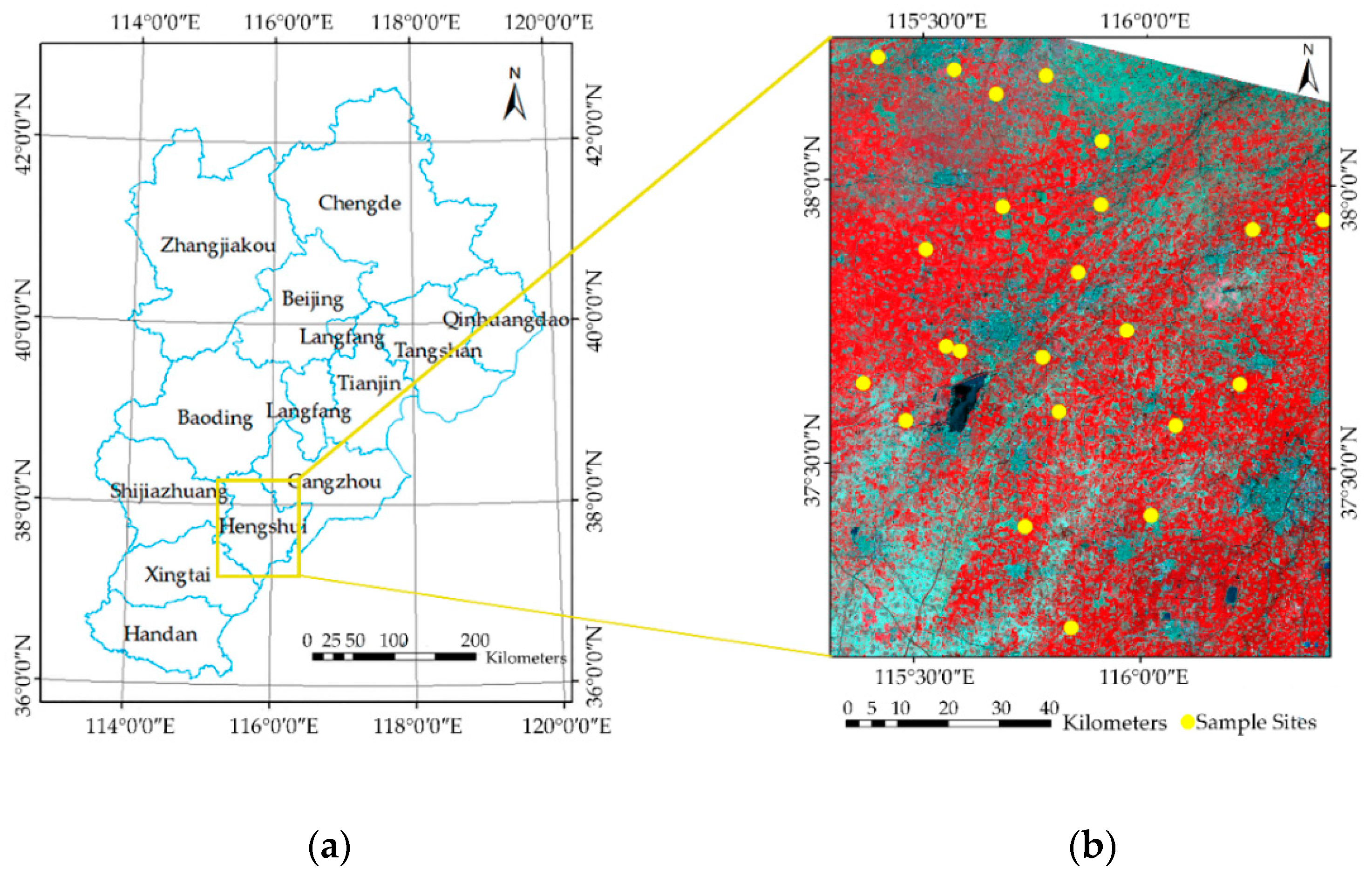
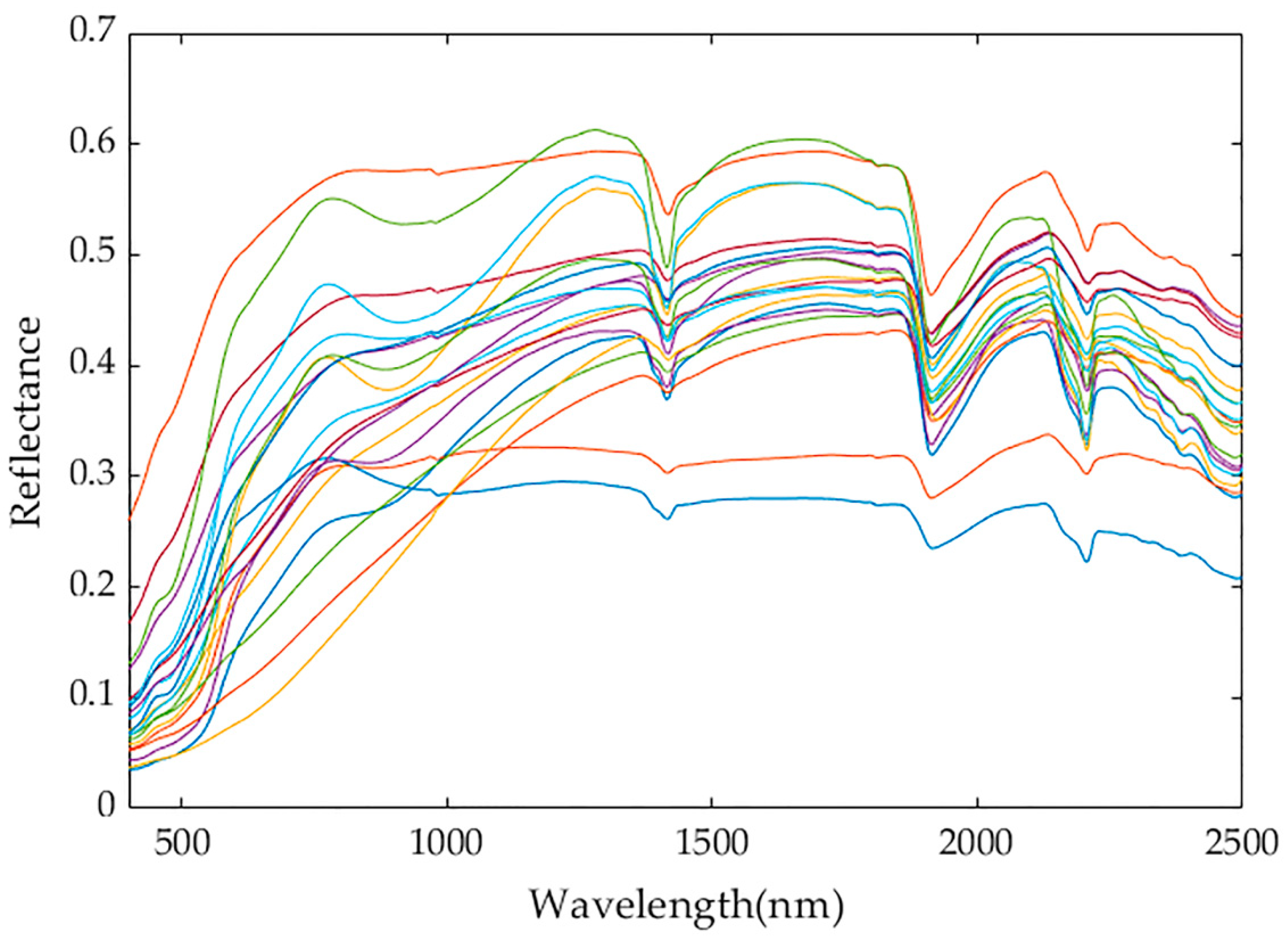
2.1. Study Area and Field Survey Data

The study area is located in Hengshui City (115°10′E~116°34′E, 37°03′N~38°23′N) of Hebei Province, China (Figure 1a). The landform is plain, with an average elevation of 23 m. The average annual temperature and precipitation are approximately 13.33 °C and 522.5 mm, respectively. Cultivated land and residential land are the main land cover types in this area.

The sample sites were distributed over the cropland in 11 counties of Hengshui (Figure 1b). The field survey data were collected for winter wheat and maize in four key crop growth periods (

Table 1. The observation periods of the field survey fractional vegetation cover (FVC).

Crop Type	The Start and End Time of Field Observation
Winter Wheat	29 March 2017 to 1 April 2017
Winter Wheat	4 May 2017 to 6 May2017
Maize	5 July 2017 to 8 July 2017
Maize	29 July 2017 to 31 July 2017

). Each collection period lasted for 2–3 days. There were two 100 m × 100 m sample sites in each county. For each sample site, five sample points with size of 30 m × 30 m were selected, including four on the corners and one at the center. Therefore, there were 110 ground truth points (GTPs) during each observation period. At each sample point, five digital images were acquired using a digital camera from the nadir, and the average of FVC extracted from these five digital images was considered as the field survey FVC at this sample point.

The FVC of a digital image was extracted by calculating the proportion of the vegetation pixel number in the total image. To eliminate the systematic bias caused by the distortion and the perspective effect of the image edge, 25% of the image edge was removed. The FVC extraction from digital image was based on an automatic shadow-resistant LABFVC (SHAR-LABFVC) algorithm, which introduced Hue Saturation Intensity (HSI) to enhance the brightness of the shadow, making sure that vegetation pixels were accurately identified over heavy shaded areas [28]. The extraction example of this algorithm used for winter wheat image (Figure 2) revealed that FVC could be effectively extracted.

2.2. Remote Sensing Data and Pre-Processing

2.2.1. GF-1 WFV Data

The GF-1 satellite is equipped with two Panchromatic/Multi-spectral (PMS) cameras and four WFV cameras. The GF-1 WFV sensors can provide multi-spectral data with a spectral range from 450 to 890 nm, including three visible bands (blue, green, red) and one near-infrared band. Although the revisit cycle of GF-1 WFV could be set as 4 days by combining the four WFV sensors, the GF-1 WFV data provided by China Centre for Resources Satellite Data and Application (CRESDA) (http://www.cresda.com/CN/) could not be used to construct time-series data with 4-day intervals due to the occasional absence of data for half a month, and the unfavorable weather conditions reduced the number of high-quality data providing continuous and effective observations for the same region. Therefore, it is necessary to generate synthetic GF-1 WFV data to fill the temporal gaps using temporal information from other remote sensing data with high-frequency observations, such as cloud-cleared MODIS data. GF-1 WFV data used in this study are listed in

Table 2. Information of the GF-1 WFV data used in this study.

Acquisition Date	Sensor Type	Tile Number
8 March 2017	WFV4	3411993
12 March 2017	WFV4	3420332
1 April 2017	WFV3	3502340, 3502339
18 April 2017	WFV3	3566875
26 April 2017	WFV4	3595448
12 May 2017	WFV3	3650209
26 June 2017	WFV1	3810592
8 July 2017	WFV2	3856572
10 August 2017	WFV3	3977545

.

The pre-processing of GF-1 WFV data included radiance calibration, atmospheric correction, and geometric correction. The DN value of the original data was converted to radiance using the following equation:

$${\mathrm{L}}_{\mathrm{e}} = \mathrm{Gain}\times \mathrm{DN}+\mathrm{Offset}$$

(1)

where ${\mathrm{L}}_{\mathrm{e}}$ is the radiance, and Gain and Offset are the calibration coefficients obtained from CRESDA (http://218.247.138.119/CN/Downloads/dbcs/11307.shtml). According to the spectral response functions of GF-1 WFV sensors provided by CRESDA, the atmospheric correction was conducted using the FLAASH method [29] based on the ENVI platform (Version 4.8). For the geometric correction, the orthographical correction was first performed using the RPC data of GF-1 WFV. Then, the precision geometric correction was performed. Because the geometric positioning of Landsat 8 data was in good consistency with the GPS values of field survey data, high-quality Landsat 8 data were selected as the reference data for ground control points selection.

2.2.2. MOD09A1 Reflectance and GLASS FVC Data

MODIS reflectance product (MOD09A1) and Global LAnd Surface Satellite (GLASS) FVC product were selected as coarse resolution data for reflectance fusion and FVC fusion, respectively. The Visible Infrared Imaging Radiometer Suite (VIIRS) on-board the Suomi National Polar-Orbiting Partnership (S-NPP) satellite, a successor for MODIS, is also a valuable coarse resolution data source. However, a mature time-series FVC product of VIIRS data has not been generated to date. Thus, MODIS and its derived FVC product (GLASS FVC) are currently more suitable for this study. MOD09A1 is an 8-day composited surface reflectance product with 500-m spatial resolution. The green (band 4), red (band1) and near-infrared bands (band 2) of MOD09A1 were used for reflectance fusion. The MOD09A1 data were reprocessed using the temporal-spatial filtering method developed by Tang et al. [30] to obtain cloud-cleared MODIS reflectance data. The GLASS FVC product was derived from the reprocessed MOD09A1 reflectance data based on the Multivariate Adaptive Regression Splines (MARS) model, which was trained using the globally distributed training samples extracted from Landsat TM and ETM+ data [31,32]. The validation results showed that GLASS FVC had good accuracy and spatio-temporal continuities [33]. The tiles and acquisition dates of MOD09A1 and GLASS FVC data selected are presented in

Table 3. Information of MOD09A1 and GLASS FVC used in this study.

Tiles	Day of Year (DOY)
H27V05	DOY65, DOY89, DOY105, DOY113, DOY117, DOY121, DOY129, DOY185, DOY209, DOY217

.

The pre-processing of MOD09A1 reflectance and GLASS FVC data were identical. First, the projection was converted from the Sinusoidal to the Universal Transverse Mercator (UTM) using the MODIS Reprojection Tool (MRT), in which the green, red and near-infrared bands of MOD09A1 were extracted simultaneously. Then, the re-projected data were clipped to match the range of the study area and resampled to 16 m spatial resolution using the cubic convolution method to meet the requirements of the fusion algorithm.

2.3. Overall Workflow

The flow chart of this study is shown in Figure 3. Strategies FC and CF were conducted, and the predicted results of these two strategies were evaluated and compared based on the field survey FVC and the FVC estimated from the actual GF-1 WFV reflectance data.

2.4. FVC Estimation Model for GF-1 WFV Data

Due to the clear physical significance, the physical method was adopted to construct the FVC estimation model for GF-1 WFV data. The complex inversion process was simplified by machine learning method in this study. Random Forest Regression (RFR) is insensitive to noise or overfitting, and less parameters need to be optimized in this method compared with other machine learning algorithms, such as Neural Networks (NNs) and Support Vector Regression (SVR). RFR also shows satisfactory accuracy in the FVC estimation using remote sensing data [34,35]. Therefore, RFR is a suitable choice for building the FVC estimation model for GF-1 WFV data.

The construction of the FVC estimation model for GF-1 WFV involved generating learning a dataset and training the RFR. First, the widely used PROSAIL model was utilized to simulate a learning dataset containing the canopy reflectance and the corresponding FVC under various vegetation conditions. Then, the RFR was trained using simulated data to model the relationship between band reflectance and FVC and was finally used to estimate FVC from GF-1 WFV data.

2.4.1. Generating Simulated Datasets Based on the PROSAIL Model

The PROSAIL model, a combination of the leaf optical property model PROSPECT [36] and the canopy reflectance model SAIL [37], has been widely used in the retrieval of vegetation biophysical parameters given its simplicity, general robustness and satisfactory performance in validation [2,13,38,39]. In this study, the version of PROSPECT-D model was selected. The hemispheric reflectance and transmission of leaves over wavelengths from 400 nm to 2500 nm can be simulated based on the PROSPECT model by providing several physiological and biochemical parameters [36]. The SAIL model with hot-spot correction [40] is a canopy Bi-directional Reflectance Distribution Function (BRDF) model to simulate the vegetation canopy reflectance under different observation conditions [37]. Since FVC is the canopy structural parameter to retrieve, the classical gap fraction described by LAI and ALA was used to convert the simulated LAI to FVC [2]. To avoid the redundant calculation and better represent land surface conditions, reasonable ranges or fixed values were given to the input parameters for the PROSAIL model based on the previous studies [35,41,42,43] (

Table 4. The ranges or values given to the parameters for the PROSAIL model.

Model	Parameters	Unit	Range	Distribution	Mean	Std.
PROSPECT	${\mathrm{C}}_{\mathrm{ab}}$	μg/cm2	20~90	Gauss	45	30
	${\mathrm{C}}_{\mathrm{m}}$	g/cm2	0.003~0.011	Gauss	0.005	0.005
	${\mathrm{C}}_{\mathrm{ar}}$	μg/cm2	4.4	-	-	-
	${\mathrm{C}}_{\mathrm{w}}$	cm	0.005~0.015	Uniform
	${\mathrm{C}}_{\mathrm{brown}}$	-	0~2	Gauss	0	3
		μg/cm2	0	-	-	-
	N	-	1.2~2.2	Gauss	1.5	0.3
SAIL	LAI	-	0~7	Gauss	2	3
	ALA	°	30~80	Gauss	60	30
	SZA	°	35	-	-	-
	VZA	°	0	-	-	-
	RAZ	°	0	-	-
	Hot	-	0.1~0.5	Gauss	0.2	0.5

).

Soil reflectance is also an important parameter for the PROSAIL model. The soil reflectance was derived from the global soil spectral library provided by the International Soil Reference and Information Center (http://www.isric.org) in this study. Because the original soil spectral data were enormous and contained redundant information, the Spectral Angle Mapper (SAM) method [44] was used to select representative soil spectral from the original data. Assuming two spectral vectors with n bands, ${\mathrm{X} = (\mathrm{x}}_1{,\mathrm{x}}_2,\cdots {,\mathrm{x}}_{\mathrm{n}})$ and ${\mathrm{Y} = (\mathrm{y}}_1{,\mathrm{y}}_2,\cdots {,\mathrm{y}}_{\mathrm{n}}),$ the spectral angle between these two vectors can be expressed as follows:

$${{\displaystyle \mathsf{\alpha }}}_{\mathrm{XY}}{ = \cos }^{-1}\left[\frac{{\displaystyle \sum _{\mathrm{i}=1}^{\mathrm{n}}\mathrm{xiyi}}}{{{\displaystyle \left({\displaystyle \sum _{\mathrm{i}=1}^{\mathrm{n}}{\mathrm{x}}_{\mathrm{i}}^2}\right)}}^{1/2}{{\displaystyle \left({\displaystyle \sum _{\mathrm{i}=1}^{\mathrm{n}}{\mathrm{y}}_{\mathrm{i}}^2}\right)}}^{1/2}}\right]$$

(2)

where ${\mathsf{\alpha }}_{\mathrm{XY}}$ represents the spectral angle between soil spectral vectors X and Y, ranging from 0 to $\mathsf{\pi }/2.$ The greater difference between the two vectors, the lager ${\mathsf{\alpha }}_{\mathrm{XY}}$ is. In this study, when ${\mathsf{\alpha }}_{\mathrm{XY}}$ is less than 0.05, these two soil spectral vectors are considered to be similar. Finally, 20 soil reflectances (Figure 4) were extracted from the original soil spectral data to characterize the possible range of soil spectral reflectances.

The reflectance of the vegetation canopy at each wavelength under different parameter combinations was calculated using PROSAIL. Then, according to the spectral response functions of GF-1 WFV sensors, resampling was conducted to simulate GF-1 WFV observations at green, red and near-infrared bands. The simulation finally generated a lookup table containing 180,000 cases of reflectances and the corresponding FVC for each WFV sensor. In total, 80% of the cases were selected as the training samples of RFR model, and the remaining 20% were selected as validation samples.

2.4.2. Random Forest Regression

The RFR algorithm [45] is an ensemble learning algorithm composed by multiple regression trees. The relationship between band reflectances and FVC can be modelled by a set of decision rules using RFR [46]. Each regression tree generates a predicted value, and the final predicted value of RFR is the average response value of all regression trees. The randomness of random forest is mainly reflected in the following two aspects: (i) Each tree is grown on the independent bootstrap sample sets extracted from the training samples randomly. (ii) A random subset of the explanatory variables is selected at each split node when constructing the splitting rules. Two parameters need to be optimized in RFR: the number of trees in random forest (${\mathrm{n}}_{\mathrm{tree}})$ and the number of band reflectances randomly extracted at each node (${\mathrm{m}}_{\mathrm{try}})$. RFR is not very sensitive to their values [47]. In this study, ${\mathrm{n}}_{\mathrm{tree}}$ was set as 500, and ${\mathrm{m}}_{\mathrm{try}}$ was set as 1/3 of the number of bands, which were the default values.

2.5. Spatio-Temporal Fusion Method for GF-1 WFV and MODIS Data

The ESTARFM proposed by Zhu et al. [24] was utilized to fuse GF-1 WFV and MODIS data. Compared with the STARFM, spatial heterogeneity was considered in this algorithm. Instead of simply assuming that the fine pixel changes are equal to the coarse pixel changes, a conversion coefficient denoting the ratio of changes between fine and coarse pixels was introduced. This modification improved the prediction accuracy in the heterogeneous region, and more spatial details could be captured. Based on this coefficient, the prediction of a GF-1 WFV pixel can be determined using Equation (3):

$$\mathrm{F}\left({\mathrm{X},\mathrm{Y},\mathrm{T}}_{\mathrm{p}}\right) = \mathrm{F}\left({\mathrm{X},\mathrm{Y},\mathrm{T}}_0\right)+\mathrm{V}(\mathrm{X},\mathrm{Y})\times (\mathrm{C}\left({\mathrm{X},\mathrm{Y},\mathrm{T}}_{\mathrm{p}}\right){-\mathrm{C}(\mathrm{X},\mathrm{Y},\mathrm{T}}_0\left)\right)$$

(3)

where F and C are the GF-1 WFV pixel value and MODIS pixel value, respectively; (X,Y) is the location of the target pixel; ${\mathrm{T}}_{\mathrm{p}}$ is the prediction date; ${\mathrm{T}}_0$ is the acquisition date of the base data; and V(X,Y) is the conversion coefficient of the target pixel.

The key step of ESTARFM is the calculation of V. To obtain the value of V, two pairs of MODIS data and GF-1 WFV data before and after the prediction time (${\mathrm{T}}_{\mathrm{m}}$ and ${\mathrm{T}}_{\mathrm{n}})$ are required. V was computed for each pixel by establishing linear regression relationship between the GF-1 WFV and MODIS pixel values of all the similar pixels in two observed pairs. The slope of the fitted line in the linear regression analysis is considered as the conversion coefficient V. Here, similar pixels are selected in a moving search window for the target pixel based on the spectral similarity. To reduce uncertainty, ESTARFM also takes full advantage of the information from these similar pixels to calculate the final prediction by giving weights to them. Similar pixels with higher spectral similarity between the coarse and fine pixels and closer spatial distance to the central pixel are considered to have greater impacts on the central pixel and given higher weights. Moreover, two predicted results were generated using the base data at ${\mathrm{T}}_{\mathrm{m}}$ and ${\mathrm{T}}_{\mathrm{n}},$ separately. The final prediction at ${\mathrm{T}}_{\mathrm{p}}$ was the combination of the two predicted results by giving weights to them. Based on the above optimizations, the predicted result can be computed as follows:

$$\mathrm{F}\left({\mathrm{X}}_{\mathrm{w}/2}{,\mathrm{Y}}_{\mathrm{w}/2}{,\mathrm{T}}_{\mathrm{p}}\right){ = \mathrm{W}}_{\mathrm{m}}{\times \mathrm{F}}_{\mathrm{m}}\left({\mathrm{X}}_{\mathrm{w}/2}{,\mathrm{Y}}_{\mathrm{w}/2}{,\mathrm{T}}_{\mathrm{p}}\right){+\mathrm{W}}_{\mathrm{n}}{\times \mathrm{F}}_{\mathrm{n}}\left({\mathrm{X}}_{\mathrm{w}/2}{,\mathrm{Y}}_{\mathrm{w}/2}{,\mathrm{T}}_{\mathrm{p}}\right)$$

(4)

where F is the final predicted result; ${\mathrm{F}}_{\mathrm{m}}$ and ${\mathrm{F}}_{\mathrm{n}}$ are the predictions generated by base data at ${\mathrm{T}}_{\mathrm{m}}$ and ${\mathrm{T}}_{\mathrm{n}},$ respectively; ${\mathrm{W}}_{\mathrm{m}}$ and ${\mathrm{W}}_{\mathrm{n}}$ are the temporal weight given to ${\mathrm{F}}_{\mathrm{m}}$ and ${\mathrm{F}}_{\mathrm{n}}$; (${\mathrm{X}}_{\mathrm{w}/2}{,\mathrm{Y}}_{\mathrm{w}/2})$ is the location of the target pixel; and $\mathrm{w}$ is the size of the moving window for the target pixel.

In this study, $\mathrm{w}$ was set as 51 × 51 pixels of GF-1 WFV, the number of similar pixels for the target pixel in the moving window was set as 20, and the number of land cover class for the selection of similar pixels was set as 4. Since there is no limitation on the number of input bands for ESTARFM, multiple reflectance bands and one FVC band can be fused using ESTARFM. Therefore, there are two fusion strategies as mentioned above to generate FVC with high spatio-temporal resolution: the strategy of fusing reflectance data (FC) and the strategy of fusing derived FVC data (CF). In some cases, the MODIS data matching the date of GF-1 WFV data cannot be found in the time series. Considering that MOD09A1 is an 8-day composited product, the MODIS data fused with GF-1 WFV data can be selected according to the composited period to which the corresponding GF-1 WFV data belong.

2.6. Validation Method

Two parts need to be validated in this study: the accuracy of the FVC estimation model for GF-1 WFV and the reliability of the fusion of GF-1 WFV and MODIS data. Assessment of the FVC estimation model was first performed based on simulated validation data derived from the PROSAIL model. Then, a direct validation comparing the field survey FVC and the FVC estimated from the actual GF-1 WFV data was conducted. To validate the reliability of the fusion result, FVC estimated from the real GF-1 WFV data and the field survey FVC were considered as the reference data. Although the aim of the spatio-temporal fusion is to predict the FVC at the time when real GF-1 WFV data could not be acquired and to compare the predicted results against the reference data, FVC was predicted on the date when the reference data were known. Therefore, the performances of strategies FC and CF were validated using two methods. The first approach was to compare the predicted result with the FVC estimated from the real GF-1 WFV data, in which visual comparison and pixel-to-pixel validation were both implemented. The second approach was to compare the predicted FVC at each sample site with the field survey FVC. To evaluate the performances quantitively, the coefficient of determination R² and Root Mean Square Error (RMSE) were calculated.

3. Results

3.1. Assessment of the GF-1 WFV FVC Estimation Model

From the validation based on the simulated data (Figure 5), the GF-1 WFV FVC estimation models for the four WFV sensors show satisfactory accuracy (R² ≥ 0.966, RMSE ≤ 0.05). Most of the scattered points are distributed along the 1:1 reference line. As the input parameter, LAI of the PROSAIL model was set as a Gaussian function distribution, and the simulated FVC also conformed to the Gaussian distribution after LAI was converted into FVC. The validation performance indicates that the RFR model is reliable and has good generalization ability to adapt to various situations.

Although there were four field survey periods, the GF-1 WFV data matching the second field survey period (4 May 2017 to 6 May 2017) was covered by cloud at the sampling locations, and there was no GF-1 WFV data acquired around the fourth field survey period (29 July 2017 to 31 July 2017). Therefore, only the field survey data collected from 29 March 2017 to 31 March 2017 and from 5 July 2017 to 8 July 2017 was used to validate the accuracy of the FVC estimation model for GF-1 WFV (Figure 6). In Hengshui City, maize in early July is in the seedling stage, whereas winter wheat is in the vigorous growth period at the end of March and the beginning of April. Thus, the FVC of winter wheat is much higher than that of maize. The fitted line with a slope of 0.973 is almost parallel to the 1:1 reference line. The validation result (R² = 0.89, RMSE = 0.071) also indicates that the GF-1 WFV FVC estimation model has reliable estimation accuracy, and the trained RFR model is robust and can be used for generating high quality FVC from GF-1 WFV reflectance data.

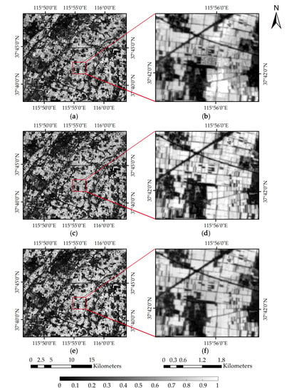
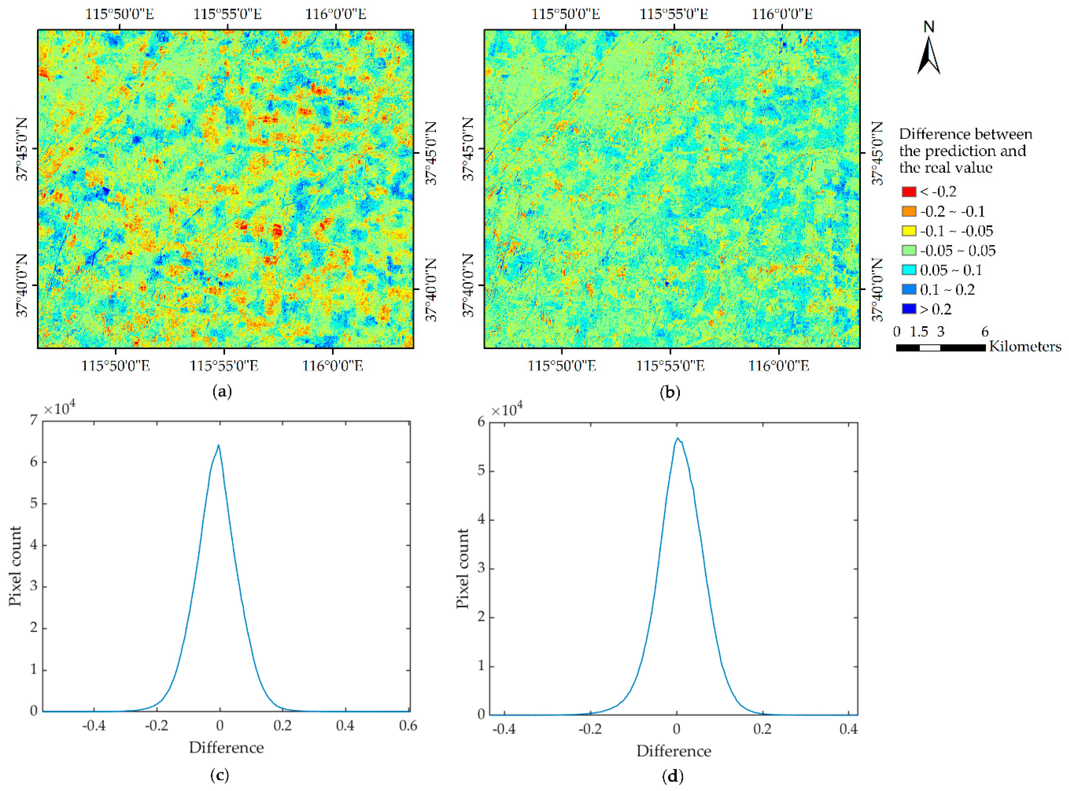
3.2. Assessment and Comparison of Strategies FC and CF

3.2.1. Assessment Based on FVC Estimated from the Actual GF-1 WFV Data

The acquisition dates of GF-1 WFV and MODIS data to fuse and the acquisition date of actual data for validation are shown in

Table 5. The acquisition dates of GF-1 WFV and MODIS data.

Dates of GF-1 WFV to Fuse	Dates of MODIS to Fuse	Predicted Date	Date of the Actual GF-1 WFV
18 April 2017	DOY105	DOY113	26 April 2017
12 May 2017	DOY129

. A subset of the study area (1590 × 1351 GF-1 WFV pixels) was selected to assess the performance of strategies FC and CF (Figure 7). Figure 8 shows the FVC prediction from strategies FC and CF and the FVC estimated from actual GF-1 WFV data. Visually, the results obtained from the two strategies both closely resemble the FVC estimated from actual data, successfully capturing most of the FVC changes. However, strategy CF performs better than strategy FC given that the patches with low FVC prediction values in the cropland near to the residential area are considerably more obvious in FC. Cropland and residential areas are the main endmembers for the mixed MODIS pixels between these two land cover types. When the residential area contributes more information to the mixed pixels, the FVC of the mixed pixels are significantly lower compared with cropland, making it easier to generate patches with low prediction after fusion. As shown in the figures presenting details of the two results, there are unrealistic areas in both strategies FC and CF, but CF generates a better prediction. For strategy FC, obvious noise is present in the predicted result. In addition, large errors are produced in the cropland in the center of the amplifying scenes (Figure 8b), and its value is significantly lower than the actual FVC. In contrast, almost no noise is present in the prediction of strategy CF.

The difference between the predicted and actual FVC data is represented by difference maps and difference histograms (Figure 9). Most of the pixels are concentrated between −0.1 and 0.1, making the histogram curves of strategies FC and CF both reach peak values when the difference is approximately 0. Pixels with differences between −0.1 and 0.1 account for 84% of the total pixels in FC, while the proportion of CF reaches 92%. Meanwhile, comparing Figure 9a and Figure 9b, it can be seen that the pure red and pure blue patches representing large deviations in FC are significantly greater in number and larger than those in CF. The areas in blue (predicted value higher than the actual FVC) are mainly buildings or fields with low FVC, whereas the areas in red (predicted value lower than the actual FVC) are mainly fields with high FVC that are near the residential areas.

To further evaluate the performances of strategies FC and CF, pixel-to-pixel validations were conducted (Figure 10). The validation accuracy indicates that both the strategies FC (R² = 0.9345, RMSE = 0.0719) and CF (R² = 0.9580, RMSE = 0.0576) show good FVC prediction accuracy, and CF performs slightly better than FC. Compared with CF, there are more points distributed far away from the 1:1 reference line in FC. There are two groups of points of FC with obvious erroneous prediction in the interval of [0.0, 0.2] and [0.8, 0.9] (Figure 10a). This phenomenon is consistent with the information shown in Figure 9. There are more pixels with large deviations in the prediction results of FC. The slope of the fitted line of CF is 1.017, which almost coincides with the 1:1 reference line. The slope of the fitted line of FC is 0.9229, which has larger difference from 1 compared with CF.

3.2.2. Assessment Based on Field Survey FVC

To assess the accuracy of strategies FC and CF using field survey data, four experiments were conducted (

Table 6. Information of the experimental data selected.

Number of Experiment	Date of GF-1 WFV	Date of MODIS	Predicted Date	Date of Field Survey Data
1	8 March 2017 12 March 2017	DOY65	DOY89	29 March 2017 to 1 April 2017
	26 April 2017	DOY113
2	18 April 2017	DOY105	DOY121	4 May 2017 to 6 May 2017
	12 May 2017	DOY129
3	8 July 2017	DOY185	DOY209	29 July 2017 to 31 July 2019
	10 August 2017	DOY217
4	26 June 2017	DOY117	DOY185	5 July 2017 to 8 July 2017
	DOY209 (Results of the No.3 Experiment)	DOY209

). In the first three experiments, actual GF-1 WFV and MODIS data were fused to predict FVC at the time when field survey data were acquired. In the No.4 Experiment, due to the absence of actual GF-1 WFV data, the second fine resolution image input to ESTARFM was the predicted result of the No.3 Experiment rather than the actual GF-1 WFV data. Because clouds covered the field survey sites in some cases, not all the field survey data were selected for the accuracy validation.

Different from the pixel-to-pixel validation results in Section 3.2.1, strategy CF (R² = 0.8138, RMSE = 0.0985) achieved more satisfactory performance than that of strategy FC (R² = 0.7173, RMSE = 0.1214) when compared with the field survey data. As is shown in Figure 11a, the scattered points of the four measurement periods in strategy FC have different degrees of deviation from the 1:1 reference line. There is a point on the horizontal axis with the coordinate of (0.1, 0). It is possible that the pixel corresponding to this point was predicted as a non-vegetation land cover type after reflectance fusion, and then the FVC value of this pixel was estimated as 0 when calculated using the FVC estimation model. All the results show that FC is instability compared to CF, which will bring greater uncertainty and higher probability of generating large errors.

Unlike the strategy FC, the sample points of strategy CF are mainly distributed near the 1:1 reference line (Figure 11b). The scattered points of the period from 5 July to 8 July appear to distribute more consistently with the 1:1 reference line than those of the other three periods. It should be noted that the predicted results of the period from 5 July to 8 July were obtained by the fusion of the actual GF-1 WFV FVC data on 26 June and the FVC fusion result of No.3 Experiment. Thus, the fusion results of No.3 Experiment were “reused”. Therefore, we can infer that reliable prediction could also be obtained by reusing the predicted results as the base data of fusion, and it is possible to utilize this “reused” method to generate long-term time-series FVC product in the future.

4. Discussion

Spatial and temporal fusion methods have been applied for the generation of NDVI and EVI time series in previous studies [25,26,27]. This study extends such fusion algorithms to the estimation of FVC time series with fine spatio-temporal resolution. Since vegetation indices, such as NDVI and EVI, are directly obtained from the band combination, the fusion results of vegetation indices were directly compared with the vegetation indices calculated from real data in previous studies [48,49], which can adequately validate the performance of the fusion. However, for vegetation parameters, the fusion results need to be validated with the ground truth to determine whether they are consistent with the actual condition. Hence, in addition to the comparison against the FVC derived from the real GF-1 WFV data, validation based on field survey data was also conducted in this study to further assess the accuracy of the fusion results.

This study indicates the feasibility of fusing GF-1 WFV and MODIS data to generate high spatio-temporal resolution FVC estimates at the GF-1 WFV scale. The results were compared for a strategy of data fusion of reflectance data (strategy FC) versus fusion of derived FVC (strategy CF). The results indicate that strategy CF outperforms FC, which is mainly reflected as follows: (i) The predicted FVC data generated by FC have large unrealistic patches, whereas this phenomenon is not obvious in CF, which better reflects the spatial details; (ii) The accuracy of CF is significantly better than that of FC with a higher R² and a smaller RMSE; (iii) The probability of generating abnormal CF values is lower. The fact that FC performs worse than CF is mainly caused by error propagation. Regarding strategy FC, the errors caused by the sensors, data pre-processing and the fusion algorithm will be further propagated to the estimation of FVC after reflectance fusion, and certain uncertainties will be generated in the process of error propagation. Although some errors are also be propagated to FVC fusion after data pre-processing in strategy CF, CF only needs to fuse one FVC band compared with FC which fuses three reflectance bands, and the impact of errors on the final predicted result is relatively smaller. In addition to the greater uncertainty of predicted results and higher probability of abnormal predicted values, the strategy FC is also limited by the type of WFV sensor. There are four WFV sensors on-board GF-1 satellites, and their spectral response functions have some minor differences. Thus, four different FVC estimation models were constructed according to the sensor type. After reflectance fusion in strategy FC, a suitable FVC estimation model should be selected for the fused data. When GF-1 data acquired from two different WFV sensors are selected as two fine-resolution base data for reflectance fusion, it is a problem when selecting the FVC estimation model for the reflectance fusion result. Regardless of which model is selected, some errors may be introduced into the final result. In addition, since FC needs to fuse three reflectance bands, the operation time required is approximately three times longer than that of CF. Therefore, in terms of computational efficiency, CF is also obviously superior to FC.

The accuracy of the fusion results is related to whether the land cover type changes [50]. The change of land cover type may lead to poorer accuracy. For the cropland, the crop type may change between two base dates of fusion. Taking the study area in this research as an example, crop grown in the same cropland changes from winter wheat to maize after July. Therefore, when applying the ESTARFM algorithm, it should be noted that the dates of the two pairs of base data should be as close as the prediction date to ensure they are in the same crop-growing season. If the spectral characteristics of vegetation at the two base time are significantly different, uncertainties would be introduced to the fusion process and further influenced the accuracy of the predicted results. When this method is extended to large-scale areas with multiple vegetation types, the base data of the fusion are relatively difficult to determine. The changes of the growing season in different local areas are not synchronized due to the differences in vegetation types. Therefore, a strategy that uses the identical base images for the entire area may not satisfy all local conditions. According to the vegetation types and the changes of the growth conditions, the large-scale region can be decomposed into several small regions. Suitable base data with acquisition dates that are close can then be selected for each small region, ensuring the dates of the base images are within the same growing season. If there are cropland, forest, grassland and other vegetation types in the area, it is recommended to focus on the changes in cropland rather than other types and divide the area mainly according to the differences between croplands. Crop type may change during several months in the same cropland, whereas this change is not obvious for forest and grassland.

The MODIS data are chosen as the coarse resolution data for the fusion. As mentioned above, VIIRS data also have potential in spatio-temporal fusion. Although an FVC estimation algorithm for VIIRS has been developed [51], the mature time-series VIIRS FVC product has not been produced, which makes VIIRS data unable to effectively fill the gaps in time series for high spatial resolution data. Therefore, the application of VIIRS data in spatio-temporal fusion can be studied in the future, and it is also worth comparing the performances of VIIRS and MODIS in the spatio-temporal fusion. Which method can generate more reliable prediction will be explored in further work.

5. Conclusions

This study evaluated the feasibility of generating high spatio-temporal resolution FVC based on the fusion of GF-1 WFV and MODIS data. The validations based on the field survey FVC and the FVC derived from the real GF-1 WFV data indicated that GF-1 WFV and MODIS data could be fused to generate high spatio-temporal resolution FVC with satisfactory accuracy. In addition, the strategies of estimating FVC from the prediction of reflectance fusion (strategy FC) and directly fusing FVC data (strategy CF) were compared, and results indicated that CF is more preferable for generating high spatio-temporal resolution FVC than FC. However, the fusion method will be limited by the huge computational cost when applied to a large region. Therefore, it is necessary to consider the parallel processing of the fusion algorithm in the future work to generate high spatio-temporal resolution FVC products for large-scale regions.

References

1. Xiao, J.; Moody, A. A comparison of methods for estimating fractional green vegetation cover within a desert-to-upland transition zone in central New Mexico, USA. Remote Sens. Environ. 2005, 98, 237–250. [Google Scholar] [CrossRef]
2. Jia, K.; Liang, S.; Gu, X.; Baret, F.; Wei, X.; Wang, X.; Yao, Y.; Yang, L.; Li, Y. Fractional vegetation cover estimation algorithm for Chinese GF-1 wide field view data. Remote Sens. Environ. 2016, 177, 184–191. [Google Scholar] [CrossRef]
3. Gitelson, A.A.; Kaufman, Y.J.; Stark, R.; Rundquist, D. Novel algorithms for remote estimation of vegetation fraction. Remote Sens. Environ. 2002, 80, 76–87. [Google Scholar] [CrossRef] [Green Version]
4. Zhang, X.; Liao, C.; Li, J.; Sun, Q. Fractional vegetation cover estimation in arid and semi-arid environments using HJ-1 satellite hyperspectral data. Int. J. Appl. Earth Obs. Geoinf. 2013, 21, 506–512. [Google Scholar] [CrossRef]
5. Carlson, T.N.; Perry, E.M.; Schmugge, T.J. Remote estimation of soil moisture availability and fractional vegetation cover for agricultural fields. Agric. For. Meteorol. 1990, 52, 45–69. [Google Scholar] [CrossRef]
6. Jiapaer, G.; Chen, X.; Bao, A. A comparison of methods for estimating fractional vegetation cover in arid regions. Agric. For. Meteorol. 2011, 151, 1698–1710. [Google Scholar] [CrossRef]
7. Niu, R.Q.; Du, B.; Wang, Y.; Zhang, L.Q.; Chen, T. Impact of fractional vegetation cover change on soil erosion in Miyun reservoir basin, China. Environ. Earth Sci. 2014, 72, 2741–2749. [Google Scholar] [CrossRef]
8. Zeng, X.B.; Dickinson, R.E.; Walker, A.; Shaikh, M.; Defries, R.S.; Qi, J.G. Derivation and Evaluation of Global 1-km Fractional Vegetation Cover Data for Land Modeling. J. Appl. Meteorol. 2000, 39, 826–839. [Google Scholar] [CrossRef]
9. Zhang, X.; Liu, X.; Zhang, M.; Dahlgren, R.A.; Eitzel, M. A review of vegetated buffers and a meta-analysis of their mitigation efficacy in reducing nonpoint source pollution. J. Environ. Qual. 2010, 39, 76–84. [Google Scholar] [CrossRef]
10. Liang, S.; Li, X.; Wang, J. Advanced Remote Sensing: Terrestrial Information Extraction and Applications; Academic Press: Cambridge, MA, USA, 2012. [Google Scholar]
11. Baret, F.; Pavageau, K.; Béal, D.; Weiss, M.; Berthelot, B.; Regner, P. Algorithm Theoretical Basis Document for MERIS Top of Atmosphere Land Products (TOA_VEG); Inra-Cseavignon: Avignon, France, 2006. [Google Scholar]
12. Schwieder, M.; Leitao, P.J.; Suess, S.; Senf, C.; Hostert, P. Estimating Fractional Shrub Cover Using Simulated EnMAP Data: A Comparison of Three Machine Learning Regression Techniques. Remote Sens. 2014, 6, 3427–3445. [Google Scholar] [CrossRef] [Green Version]
13. Si, Y.; Schlerf, M.; Zurita-Milla, R.; Skidmore, A.; Wang, T. Mapping spatio-temporal variation of grassland quantity and quality using MERIS data and the PROSAIL model. Remote Sens. Environ. 2012, 121, 415–425. [Google Scholar] [CrossRef]
14. Mu, X.; Song, W.; Gao, Z.; McVicar, T.R.; Donohue, R.J.; Yan, G. Fractional vegetation cover estimation by using multi-angle vegetation index. Remote Sens. Environ. 2018, 216, 44–56. [Google Scholar] [CrossRef]
15. Baret, F.; Hagolle, O.; Geiger, B.; Bicheron, P.; Miras, B.; Huc, M.; Berthelot, B.; Niño, F.; Weiss, M.; Samain, O. LAI, fAPAR and fCover CYCLOPES global products derived from VEGETATION: Part 1: Principles of the algorithm. Remote Sens. Environ. 2007, 110, 275–286. [Google Scholar] [CrossRef] [Green Version]
16. Roujean, J.L.; Lacaze, R. Global mapping of vegetation parameters from POLDER multiangular measurements for studies of surface-atmosphere interactions: A pragmatic method and its validation. J. Geophys. Res. Atmos. 2002, 107. [Google Scholar] [CrossRef]
17. Zou, J.; Lan, J.; Shao, Y. A hierarchical sparsity unmixing method to address endmember variability in hyperspectral image. Remote Sens. 2018, 10, 738. [Google Scholar] [CrossRef]
18. Shao, Y.; Lan, J.; Zhang, Y.; Zou, J. Spectral Unmixing of Hyperspectral Remote Sensing Imagery via Preserving the Intrinsic Structure Invariant. Sensors 2018, 18, 3528. [Google Scholar] [CrossRef] [PubMed]
19. Gutman, G.; Ignatov, A. The derivation of the green vegetation fraction from NOAA/AVHRR data for use in numerical weather prediction models. Int. J. Remote Sens. 1998, 19, 1533–1543. [Google Scholar] [CrossRef]
20. Kimes, D.S.; Knyazikhin, Y.; Privette, J.; Abuelgasim, A.; Gao, F. Inversion methods for physically-based models. Remote Sens. Rev. 2000, 18, 381–439. [Google Scholar] [CrossRef]
21. Baret, F.; Weiss, M.; Lacaze, R.; Camacho, F.; Makhmara, H.; Pacholcyzk, P.; Smets, B. GEOV1: LAI and FAPAR essential climate variables and FCOVER global time series capitalizing over existing products. Part1: Principles of development and production. Remote Sens. Environ. 2013, 137, 299–309. [Google Scholar] [CrossRef]
22. Mizuochi, H.; Hiyama, T.; Ohta, T.; Fujioka, Y.; Kambatuku, J.R.; Iijima, M.; Nasahara, K.N. Development and evaluation of a lookup-table-based approach to data fusion for seasonal wetlands monitoring: An integrated use of AMSR series, MODIS, and Landsat. Remote Sens. Environ. 2017, 199, 370–388. [Google Scholar] [CrossRef]
23. Gao, F.; Masek, J.; Schwaller, M.; Hall, F. On the blending of the Landsat and MODIS surface reflectance: Predicting daily Landsat surface reflectance. IEEE Trans. Geosci. Remote Sens. 2006, 44, 2207–2218. [Google Scholar]
24. Zhu, X.; Chen, J.; Gao, F.; Chen, X.; Masek, J.G. An enhanced spatial and temporal adaptive reflectance fusion model for complex heterogeneous regions. Remote Sens. Environ. 2010, 114, 2610–2623. [Google Scholar] [CrossRef]
25. Walker, J.; De Beurs, K.; Wynne, R. Dryland vegetation phenology across an elevation gradient in Arizona, USA, investigated with fused MODIS and Landsat data. Remote Sens. Environ. 2014, 144, 85–97. [Google Scholar] [CrossRef]
26. Meng, J.; Du, X.; Wu, B. Generation of high spatial and temporal resolution NDVI and its application in crop biomass estimation. Int. J. Digit. Earth 2013, 6, 203–218. [Google Scholar] [CrossRef]
27. Jia, K.; Liang, S.; Zhang, L.; Wei, X.; Yao, Y.; Xie, X. Forest cover classification using Landsat ETM+ data and time series MODIS NDVI data. Int. J. Appl. Earth Obs. Geoinf. 2014, 33, 32–38. [Google Scholar] [CrossRef]
28. Song, W.; Mu, X.; Yan, G.; Huang, S. Extracting the green fractional vegetation cover from digital images using a shadow-resistant algorithm (SHAR-LABFVC). Remote Sens. 2015, 7, 10425–10443. [Google Scholar] [CrossRef]
29. Cooley, T.; Anderson, G.P.; Felde, G.W.; Hoke, M.L.; Ratkowski, A.J.; Chetwynd, J.H.; Gardner, J.A.; Adler-Golden, S.M.; Matthew, M.W.; Berk, A. FLAASH, a MODTRAN4-based atmospheric correction algorithm, its application and validation. Proceedings of IEEE International Geoscience & Remote Sensing Symposium, Toronto, ON, Canada, 24–28 June 2002. [Google Scholar]
30. Tang, H.; Yu, K.; Hagolle, O.; Jiang, K.; Geng, X.; Zhao, Y. A cloud detection method based on a time series of MODIS surface reflectance images. Int. J. Digit. Earth 2013, 6, 157–171. [Google Scholar] [CrossRef]
31. Jia, K.; Yang, L.; Liang, S.; Xiao, Z.; Zhao, X.; Yao, Y.; Zhang, X.; Jiang, B.; Liu, D. Long-Term Global Land Surface Satellite (GLASS) Fractional Vegetation Cover Product Derived From MODIS and AVHRR Data. IEEE J. Sel. Top. Appl. Earth Obs. Remote Sens. 2019, 12, 508–518. [Google Scholar] [CrossRef]
32. Yang, L.; Jia, K.; Liang, S.; Liu, J.; Wang, X. Comparison of four machine learning methods for generating the GLASS fractional vegetation cover product from MODIS data. Remote Sens. 2016, 8, 682. [Google Scholar] [CrossRef]
33. Jia, K.; Liang, S.; Wei, X.; Yao, Y.; Yang, L.; Zhang, X.; Liu, D. Validation of Global LAnd Surface Satellite (GLASS) fractional vegetation cover product from MODIS data in an agricultural region. Remote Sens. Lett. 2018, 9, 847–856. [Google Scholar] [CrossRef]
34. Campos-Taberner, M.; Moreno-Martínez, Á.; García-Haro, F.; Camps-Valls, G.; Robinson, N.; Kattge, J.; Running, S. Global estimation of biophysical variables from google earth engine platform. Remote Sens. 2018, 10, 1167. [Google Scholar] [CrossRef]
35. Wang, B.; Jia, K.; Liang, S.; Xie, X.; Wei, X.; Zhao, X.; Yao, Y.; Zhang, X. Assessment of Sentinel-2 MSI Spectral Band Reflectances for Estimating Fractional Vegetation Cover. Remote Sens. 2018, 10, 1927. [Google Scholar] [CrossRef]
36. Jacquemoud, S.; Baret, F. PROSPECT: A model of leaf optical properties spectra. Remote Sens. Environ. 1990, 34, 75–91. [Google Scholar] [CrossRef]
37. Verhoef, W. Light scattering by leaf layers with application to canopy reflectance modeling: The SAIL model. Remote Sens. Environ. 1984, 16, 125–141. [Google Scholar] [CrossRef] [Green Version]
38. Darvishzadeh, R.; Skidmore, A.; Schlerf, M.; Atzberger, C. Inversion of a radiative transfer model for estimating vegetation LAI and chlorophyll in a heterogeneous grassland. Remote Sens. Environ. 2008, 112, 2592–2604. [Google Scholar] [CrossRef]
39. Duan, S.B.; Li, Z.L.; Wu, H.; Tang, B.H.; Ma, L.; Zhao, E.; Li, C. Inversion of the PROSAIL model to estimate leaf area index of maize, potato, and sunflower fields from unmanned aerial vehicle hyperspectral data. Int. J. Appl. Earth Obs. Geoinf. 2014, 26, 12–20. [Google Scholar] [CrossRef]
40. Kuusk, A. The hot spot effect in plant canopy reflectance. In Photon-Vegetation Interactions; Myneni, R.B., Ross, J., Eds.; Springer: Berlin/Heidelberg, Germany; pp. 139–159. [CrossRef]
41. Feret, J.B.; François, C.; Asner, G.P.; Gitelson, A.A.; Martin, R.E.; Bidel, L.P.; Ustin, S.L.; Le Maire, G.; Jacquemoud, S. PROSPECT-4 and 5: Advances in the leaf optical properties model separating photosynthetic pigments. Remote Sens. Environ. 2008, 112, 3030–3043. [Google Scholar] [CrossRef]
42. Scurlock, J.; Asner, G.; Gower, S. Worldwide Historical Estimates of Leaf Area Index, 1932–2000; ORNL/TM-2001/268; Oak Ridge National Laboratory: Oak Ridge, TN, USA, 2001; Volume 34. [Google Scholar]
43. Weiss, M.; Baret, F.; Smith, G.; Jonckheere, I.; Coppin, P. Review of methods for in situ leaf area index (LAI) determination: Part II. Estimation of LAI, errors and sampling. Agric. For. Meteorol. 2004, 121, 37–53. [Google Scholar] [CrossRef]
44. Dennison, P.E.; Halligan, K.Q.; Roberts, D.A. A comparison of error metrics and constraints for multiple endmember spectral mixture analysis and spectral angle mapper. Remote Sens. Environ. 2004, 93, 359–367. [Google Scholar] [CrossRef]
45. Breiman, L. Random forests. Mach. Learn. 2001, 45, 5–32. [Google Scholar] [CrossRef]
46. Hutengs, C.; Vohland, M. Downscaling land surface temperatures at regional scales with random forest regression. Remote Sens. Environ. 2016, 178, 127–141. [Google Scholar] [CrossRef]
47. Liaw, A.; Wiener, M. Classification and regression by randomForest. R News 2002, 2, 18–22. [Google Scholar]
48. Knauer, K.; Gessner, U.; Fensholt, R.; Kuenzer, C. An ESTARFM fusion framework for the generation of large-scale time series in cloud-prone and heterogeneous landscapes. Remote Sens. 2016, 8, 425. [Google Scholar] [CrossRef]
49. Olexa, E.M.; Lawrence, R.L. Performance and effects of land cover type on synthetic surface reflectance data and NDVI estimates for assessment and monitoring of semi-arid rangeland. Int. J. Appl. Earth Obs. Geoinf. 2014, 30, 30–41. [Google Scholar] [CrossRef]
50. Dewen, C.; Niu Zheng, W.L. Adaptability research of spatial and temporal remote sensing data fusion technology in crop monitoring. Remote Sens. Technol. Appl. 2013, 27, 927–932. [Google Scholar]
51. Liu, D.; Yang, L.; Jia, K.; Liang, S.; Xiao, Z.; Wei, X.; Yao, Y.; Xia, M.; Li, Y. Global Fractional Vegetation Cover Estimation Algorithm for VIIRS Reflectance Data Based on Machine Learning Methods. Remote Sens. 2018, 10, 1648. [Google Scholar] [CrossRef]
Figure 1. The geographic location of the whole study area is represented by the yellow rectangle in the left figure (a). The distribution of the sample sites is shown by the yellow points on the standard false color composited GaoFen-1 Wide Field View (GF-1 WFV) data (b).
Remotesensing 11 02324 g001
Figure 2. An example of FVC extraction from a digital image for winter wheat. The left picture is the original camera image (a), and the right picture is the corresponding extraction result (b).
Remotesensing 11 02324 g002
Figure 3. The flow chart of this study.
Remotesensing 11 02324 g003
Figure 4. The final extracted 20 soil reflectance curves.
Remotesensing 11 02324 g004
Figure 5. Validation based on the simulated data for GF-1 WFV 1 (a), GF-1 WFV 2 (b), GF-1 WFV 3 (c) and GF-1 WFV 4 (d).
Remotesensing 11 02324 g005
Figure 6. Validation based on field survey FVC.
Remotesensing 11 02324 g006
Figure 7. Standard false colour composited MODIS surface reflectance (upper row) data and corresponding GF-1 WFV surface reflectance (lower row) data.
Remotesensing 11 02324 g007
Figure 8. Actual FVC data on 26 April 2017 (c) and its predicted results based on the strategy of fusing reflectance data (FC) (a) and the strategy of fusing derived FVC (CF) (e). The right column images (b,d,f) show the details of the region marked in the left column images.
Remotesensing 11 02324 g008
Figure 9. Difference maps of the strategy of fusing reflectance data (FC) (a) and the strategy of fusing derived FVC (CF) (b), and difference histograms of FC (c) and CF (d).
Remotesensing 11 02324 g009
Figure 10. Density scatter plots of the FVC estimated from the actual GF-1 WFV data and the prediction generated by the strategy of fusing reflectance data (FC) (a) and the strategy of fusing derived FVC data (CF) (b).
Remotesensing 11 02324 g010
Figure 11. Validation of the prediction from FC (a) and CF (b) based on the field survey FVC data.
Remotesensing 11 02324 g011