1. Introduction
As floods presently rival earthquakes and hurricanes in terms of economic losses [
1], insurance companies face the problem of a substantial increase in flood claims. Their frequency in Germany and central Europe has increased by a factor of two since 1980 [
2]. In 2013, around 45% of the insured losses derived from inland flooding. To improve their services, insurance companies require detailed global and national disaster impact databases to identify areas vulnerable to flooding and to support parametric insurance, i.e., to trigger payouts in case of emergency using pre-defined criteria. Several international Earth Observation (EO) initiatives have set up a research and development agenda to propose new products to serve this user community and more in general to improve the services provided for crisis response and mitigation. For example, the Working group on Disasters of the Committee on Earth Observation Satellites (CEOS) highlighted the need to exploit the full potential of new EO data sets to support flood management in its various phases [
3]. In this context, SAR data play a major role in operational services for flood risk management thanks to their high sensitivity to water and the ability to provide data during day and night, regardless of cloud cover. Nowadays, several satellite constellations, such as COSMO-SkyMed (CSK) [
4], TerraSAR-X (TSX) [
5] and Sentinel-1 (S-1) allow for a considerable reduction in the revisit time of satellite images, which is an important requirement stated by the Disaster Working group.
Many studies have demonstrated that SAR systems are suitable tools for floodwater mapping on bare soil or scarcely vegetated areas [
6,
7,
8,
9,
10], where the water has a well-defined backscattering signature [
11]. Water bodies appear as dark areas in SAR images, being smooth surfaces that typically reflect the radar signal in the specular direction away from the antenna, thereby producing a very low backscatter. For this reason, a single radar observation of a flood can detect floodwater in such an environment [
7,
12,
13], although change detection approaches are often used to mask out permanent water or false alarms caused by shadows or smooth surfaces such as tarmac [
8,
14,
15]. Indeed, the use of SAR data is nowadays well-established in operational flood management thanks to automatic algorithms able to generate floodwater maps in near real-time (NRT) [
16,
17,
18]. Although in recent years much progress has been made in the development of NRT floodwater mapping procedures, the detection of inundation in complex environments, such as vegetated and urban areas, still requires further studies [
19,
20,
21,
22,
23,
24,
25,
26]. This is because radar signatures of such targets may be quite complex to predict and are often ambiguous. Other challenges that may be encountered are related to atmospheric conditions, heavy precipitation, and high winds, inducing surface roughening, which can cause misdetection due to the reduced contrast between backscatter from flooded and non-flooded soils [
27].
The presence of water in urban areas, e.g., on a road in front of a building, can be detected thanks to a significant enhancement of the double-bounce scattering mechanism, as the smooth and high permittivity water increases the surface reflectivity [
19]. The double-bounce increase, due to the presence of floodwater, may not be high enough if the building facades are not parallel to the SAR flight direction. The Interferometric SAR (InSAR) coherence, ρ, provided by Very High-Resolution (VHR) SAR data, has been used to reduce under detection in urban areas [
21,
22]. Also, the bistatic InSAR coherence, from TanDEM-X, has shown some potentiality for more accurate floodwater mapping in a complex landscape with urban and vegetation areas [
28]. The high sensitivity of ρ to surface changes is well-documented and enables the detection of damages caused by catastrophic events such as volcano eruptions, earthquakes, and floods [
29,
30,
31,
32,
33]. While the usefulness of ρ for detecting water on bare soils has been demonstrated in several studies [
33,
34], first results of a successful exploitation of this feature, derived from VHR SAR data for detecting water in urban areas, have only recently been reported [
21,
22,
28].
This paper presents an urban floodwater mapping experiment that considers for the first time 20 m S-1 images and is largely built upon recent findings concerning urban flood detection using VHR SAR data. The experiment aims to introduce and test a novel approach that is based on two fundamental processing steps: the first one exploits a multi-pass technique to detect areas of double-bounce in an urban environment; the second one uses the change of ρ within those areas to detect the inundated pixels. The novel contributions that this paper brings, with respect to current literature on floodwater mapping, are the following. First, the approach is totally self-consistent, that is, it does not need sources of data other than SAR, such as the land cover maps and/or VHR optical data that are generally used to identify urban areas. This is important for operational purposes, since ancillary data cannot always be available. Secondly, and for the first time, the approach exploits the S-1 SAR data to map urban floods. These pave the way for future operational floodwater mapping algorithms broadened to urban areas (typically masked in current approaches), despite the moderate spatial resolution of S-1 images. To verify to what extent the moderate resolution (20 m) of the default Interferometric Wide Swath (IW) S-1 products could represent a critical point for the proposed approach, the ρ feature was also extracted at 5 m, taking advantage of the availability of Strip Map (SM) data. The high sensitivity of the coherence to the presence of water within building areas is investigated in the framework of Hurricane Harvey, which hit the metropolitan area of Houston, Texas in August 2017.
The paper is organized as follows:
Section 2 describes the proposed methodology and the importance of SAR double-bounce effects for detecting flooded buildings. Details about the dataset are given in
Section 3.
Section 4 presents the results, while
Section 5 contains the discussion. Finally,
Section 6 gives the conclusions.
2. Assumptions and Methods
The VHR SAR missions such as CSK and TSX gave an important boost to the identification of floods in urban environments. The increased resolution of SAR X-band sensors up to one meter allows the identification of different scattering mechanisms that are characteristic of a building, enabling to isolate the one that can provide most useful information about the presence or not of water, i.e., the double-bounce. The double-bounce is due to the dihedral reflector composed of the building facade and its surrounding ground area. At metric resolution, it produces a very bright line that appears on the side of the wall that is illuminated by the radar [
35]. It is worth mentioning that the length of the double-bounce path is equal to the slant range of the intersection between the ground and the front wall of the building. Even if the building is surrounded by asphalt surfaces that are as smooth as water surfaces, the increase of reflectivity due to the high dielectric constant of the water implies a considerable increase of the double-bounce return. Therefore, TSX images (3 m resolution) were used in conjunction with a high-resolution light detection and ranging (LiDAR) height map of the urban area [
19]. The position of the double-bounce areas was first extracted using a SAR simulator. Then, the predictions from an electromagnetic scattering model were compared to radar observations of double-bounce backscattering enhancement to detect floodwater [
19].
The increase of the double-bounce backscatter is mainly related to the geometric arrangement of the SAR line of sight (LoS) and the building facade. The increase of the backscatter is high when the LoS is orthogonal to the horizontal alignment of the building facade, while it rapidly decreases moving away from the orthogonal direction. The SAR LoS that is unfavorable with respect to the building facade was highlighted in Pulvirenti et al. [
22] as a possible source of under-detection when relying only on SAR intensity. In Chini et al. [
21], a decrease of ρ was observed using VHR CSK X-band images of the flood event caused by the tsunami that hit Japan on 2011. This was tentatively associated with the presence of standing water. Pulvirenti et al. [
22] further developed the idea using a flood event that occurred in Italy in 2014 and introduced ρ as a solution to enable the detection of water in the areas that include such double-bounce objects. The method relayed on VHR CSK data and demonstrated its capability to significantly reduce the under-detection committed when only SAR intensity images were used. The rationale is that an urban settlement is a very steady target characterized by high ρ, even at large temporal baselines, and the appearance of floodwater implies a significant decrease of the coherence between pairs of VHR images.
For lower resolution SAR data, ρ has not yet been considered. This may be due to the lower repeat cycle of past satellites and the high temporal baseline between acquisitions. This is an important factor for decreasing ρ, especially at lower spatial resolution. In fact, in addition to the double-bounce effect, other scattering mechanisms from different land cover classes (e.g., vegetation) may occur within an individual pixel. Moreover, the spatial baseline can also cause a decrease of ρ with the increase of its perpendicular component [
36].
Indeed, the SAR spatial resolution plays an important role on the paradigm definition of how buildings are represented, what urban areas look like and consequently how changes can be detected. In VHR images, the double-bounce can be identified as the only contribution in a pixel, while in medium resolution images it can be mixed with contributions from other target categories. In the latter case, the other scattering mechanisms that take place can mask the double-bounce, thus attenuating its main characteristics, i.e., the coherence in time and the high-intensity value. The enhanced observational capabilities of the C-band S-1 mission [
37] reduce the drawbacks of previous moderate resolution SARs and potentially enable a more accurate detection of floodwater in urban areas. Indeed, the high repeat cycle (i.e., small temporal baseline) and the relatively narrow orbit tube (i.e., small perpendicular interferometric baseline) are all characteristics that provide new momentum for the development of innovative automatic urban floodwater mapping algorithms. From the results obtained using VHR SAR data and given the current availability of systematic acquisitions of medium resolution SAR data, we hypothesize that is now possible to detect floods in urban areas using SAR medium resolution data.
The ρ feature is defined as the normalized cross correlation between an interferometric pair of SAR images and it is related to the change in the spatial arrangement of the scatterers within a pixel [
29], and thus to geometric changes in the scene. An interferogram and its ρ can be built using either two images taken before the event (pre-event coherence, ρ
pre) or with one before and one during the flood event (co-event coherence, ρ
co). Given that urban areas are usually coherent in time, especially with respect to the double-bounce feature, areas where ρ
co decreases with respect to ρ
pre can be considered as subject to changes. Nevertheless, a thoughtful investigation of causes triggering the drop-off must be carried out, as numerous factors may influence ρ. Zebker & Villasenor [
36] highlighted the spatial baseline, the rotation of the target between observations and the temporal baseline as the main sources of the image decorrelation. It is obvious that the latter factor is the one enabling the detection of water appearing between buildings, while the former must be accounted to avoid false alarms. Indeed, the increase of the spatial baseline, in particular its perpendicular component, implies a decrease of ρ, thus reducing the difference between ρ
pre and ρ
co. The effect of the perpendicular baseline is even more important in urban areas, where the geometrical complexity of structures accentuates the effect [
38]. Changing vegetation is usually another important source of false alarms. To reduce such effects, it is recommended to compute ρ using pairs of images that were acquired close in time, i.e., with a short temporal baseline.
With decametric spatial resolution data, such as the 20 m S-1 IW data, the dominant scattering mechanism is still the double-bounce from buildings. However, contributions from other scatterers in the same pixel are expected and other decorrelation factors thus must be considered. Fortunately, the ρ degradation due to changes in the spatial and temporal baselines is reduced when considering S-1 SAR data. S-1 has a small and well-controlled orbital tube of 50 m, resulting in a small spatial baseline between image pairs that is, in the worst-case, equal to 100 m. The S-1 orbit cycle is 12 days and when considering just one satellite, interferometric couples are thus also available every 12 days. With the two satellites currently available, the temporal baseline is reduced to 6 days. The short revisit time is another factor that helps containing the risk of undesired ρ decrease.
2.1. InSAR Coherence Floodwater Mapping in Urban Areas
Based on the previous considerations, it is important to isolate the pixels that are dominated by the double-bounce mechanism. Furthermore, it is important to optimally exploit the S-1 frequent revisit with constant geometry. The proposed algorithm is therefore composed of two main steps: (1) prior identification of the double-bounce features in the SAR images using a multi-temporal technique; (2) detection of the ρ drop-off in the previously detected double-bounce map.
The method is based on a multi-pass approach exploiting a stack of interferometric acquisitions. The coherence map between each consecutive pair of images is extracted using a square moving window. Given t
0, i.e.
, the date of the image acquired during the flood event, we denote with ρ
co the coherence of the image pair acquired on t
0 and t
−1, and ρ
pre the one with images acquired on t
−1 and t
−2. We proceed in the same way to generate coherence maps from previous images of the stack.
Figure 1 shows the overall process, summarizing the algorithm steps. Step 1 allows the double-bounce map to be extracted, i.e.
, the building footprints, and will be described in detail in the next subsection (red blocks in
Figure 1). Step 2 combines the double-bounce map and the change of ρ
pre–ρ
co (dark blue blocks in
Figure 1). The underlying assumption is that urban areas affected by a flood have ρ
co < ρ
pre.
To provide a more exhaustive analysis of the event and to frame the new findings in a more general context, flooded bare soils have also been mapped using the algorithm proposed by Chini et al. [
16]. The associate processing module is displayed in the “bare soil flood mapping” blocks in
Figure 1 (light blue). It is based on an adaptive thresholding approach, which at the same time exploits multi-temporal information through change detection and contextual information through region-growing. It makes use of two images: one acquired during the flood event and one from before the event started. The algorithm is operational and available on the on ESA-Grid Processing on Demand (G-POD) platform under the HASARD service [
39].
2.2. Building Detection
To extract the double-bounce objects, we use an approach developed for mapping buildings at the global scale by means of S-1 data and proposed by Chini et al. [
40]. It is based on a hierarchical split-based approach described in Chini et al. [
16]. In the following paragraph, only the main underlying principles are summarized, and we refer to the relevant bibliography for details.
The method in Chini et al. [
40] is based on the fact that in the co-polarization channel, buildings are characterized by a high backscattering, as well a high degree of correlation in time between images. To increase the potential for detecting buildings when the LoS is not orthogonal to the building facade, cross-polarization backscattering is also used, as it rises when rotated dihedrals are present [
41]. High backscattering values can also occur in the case of vegetation. In the cross-polarization channel, the high backscattering values rise when the volumetric scattering is dominant, while in the co-polarization channel, high vegetation backscatter is associated with the increase of double-bounce, e.g., when water beneath vegetation is present, as exemplified by Pierdicca et al. [
26] for rice fields. To cope with false alarms generated by vegetated areas, the algorithm exploits ρ. Indeed, ρ has a contrasting behavior in vegetated and built-up areas, respectively, as buildings are stable structures, unlike vegetation. Another risk of a false alarm is caused by the layover in mountainous areas. By means of a DEM and the geometry of the SAR acquisition, the local incidence angle (LIA) is computed and the layover areas are masked out [
42].
The algorithm is composed of two steps: (i) discrimination of bright pixels in co- and cross-polarization channels, making use of a statistical modeling-based adaptive thresholding approach; (ii) removal of false alarms by using ρ and the LIA.
When handling SAR data, it is worth emphasizing the importance of accounting for speckle noise that is known to hamper, in general, a straightforward image classification when only using backscatter values on a pixel basis. In Chini et al. [
40] a temporal averaging is adopted, by exploiting the availability of the S-1 temporal series with a frequency of up to 6 days. The temporal average is performed on a stack of images from the same orbit and acquired at different times. Its main advantage is that, contrary to the multi-looking and textural approaches that decrease the spatial resolution, the speckle is reduced without decreasing resolution. Considering that we are interested in classifying a temporally coherent target, i.e., buildings, this type of approach is sensible. The algorithm generates building maps at the highest possible resolution, i.e., that of the sensor, with a temporal resolution of a few months. Similarly, ρ values extracted from the successive interferometric image pairs are averaged to obtain the temporal average coherence, TACvv, which is used to mask out bright vegetation.
In summary, the following steps constitute the overall procedure:
- (1)
Generate the temporal average intensity (TAI) using 12 different images of the co- and cross-polarization backscattering (TAIVV and TAIVH) and the TACVV separately;
- (2)
Remove layover areas using LIA;
- (3)
Identify the bright pixels from TAI
VV and TAI
VH that are representative of buildings by making use of a hierarchical split-based approach (HSBA, Chini e al. [
16]);
- (4)
Filter false alarms from the built-up area maps by considering only TACVV above a threshold;
- (5)
Merge the two built-up area maps corresponding to TAIVV and TAIVH using a logical OR function.
This approach produces a resulting map at the spatial resolution of the SAR sensor because it identifies bright pixels using TAIVV and TAIVH, whose resolution is that of the SAR; TACVV has a worse spatial resolution, equal to the size of the moving window used for computing the coherence, but it is only used to reduce the false alarm rate. Then, for urban areas where an important amount of vegetation is present, the vegetation could produce a decrease of coherence, leading to the removal of buildings from the final classification. Consequently, some under-detection can occur, but the resolution of the building map remains that of the TAIs images.
The algorithm in step (3) is extensively described in Chini et al. [
16]. It is a combination of histogram thresholding and region-growing and requires the calibration of the probability density function (PDF) attributed to the double-bounce class. The parametric binarization of an image to separate the double-bounce class from its background becomes challenging when the class of interest occupies only a small fraction of the whole image. In the algorithm, a hierarchical tiling approach based on statistical modeling has been introduced to identify regions of the image where the PDFs from the double-bounce and background classes can be parameterized more reliably and accurately. The size of the tiles depends on the possibility of parameterizing the PDFs attributed to two different classes. The final objective of the method is to define PDFs for two classes (i.e., the double-bounce and its background).
3. Test Case and Dataset
Hurricane Harvey hit Texas in August and September 2017, causing major damage in large areas of Houston, the fourth largest city in the United States. In a four-day period, unprecedented amounts of rainfall accumulated over Eastern Texas and Louisiana, following the Category 4 hurricane Harvey’s first landfall on 25 August 2017 on San Jose Island, Texas. After hitting the Texas mainland on the same day, Harvey weakened to a tropical storm and its speed reduced. As it was only progressing slowly, the amount of rainfall in the region became extremely high and the volume of water took days to drain through rivers, causing widespread catastrophic flooding, most notably in the Houston metropolitan area. The local National Weather Service office in Houston observed daily rainfall accumulations of 370 mm and 4018 mm on August 26 and 27, respectively. A total precipitation of 1539 mm in the city of Nederland in southeast Texas, makes Hurricane Harvey the wettest tropical cyclone on record in the United States [
43]. As a result, the Houston bayous burst their banks for several days, which led to substantial large-scale flooding, especially to the north and east of the Houston area. The total economic loss from the event amounted to about US
$125 billion, with more than 30,000 people evacuated from their homes, more than 17,000 rescues prompted and 106 confirmed deaths in the United States. Hurricane Harvey ties with Hurricane Katrina (2005) as the costliest tropical cyclone on record [
44].
Thanks to the systematic acquisition of EO images of this area, the amount of data acquired during Harvey (as part of the activation of the International Charter Space and Major Disasters) has reached an unprecedented level. Here we make use of S-1 images acquired over the metropolitan area of Houston on 30 August 2017, when the flooding was still ongoing and close to its peak, as well as images acquired before the event. On August 30, S-1 operated in both SM and IW mode, making it possible to test the proposed algorithm for two different spatial resolutions, 5 m and 20 m, respectively. For both acquisition modes, images acquired before the catastrophic event started are also available. The IW image covers the entire Houston area, whereas the SM ones, with a smaller swath, cover the central and eastern part of the city. All images are available in the Single Look Complex (SLC) mode (see
Figure 2).
With respect to SAR intensity, we use a pair of images consisting of a pre-flood, denoted also as ‘reference image’, and a post-flood image.
Table 1 provides details about the exact acquisition time of each image and the corresponding characteristics. The following pre-processing steps are applied to each image: multi-looking, terrain correction using a DEM, radiometric calibration, and geocoding. The multi-looking window is 4 × 1 in case of IW images, to get a square pixel of 20 m and the higher possible spatial resolution. For the SM mode, we do not perform the multi-looking because the pixel is already square, 5 × 5 m, and we want to preserve the spatial resolution. The Refined Lee speckle filter is also applied to reduce the noise level of the intensity images. In addition to the SAR intensity, we also compute ρ maps using images acquired before and during the flood event, as ρ
pre-IW, ρ
pre-SM and ρ
co-IW, ρ
co-SM. Firstly, the SAR interferogram is generated from the SLC image pairs and then ρ is estimated by using a moving window of 9 × 9 pixels. All ρs are then geocoded and resampled over the same spatial grid of the intensity images. All details are summarized in
Table 2.
As described in
Section 2.2, we make use of the S-1 multi-temporal intensity and ρ series to generate the building maps from SAR S-1 data. For this purpose, a stack of 12 SAR images acquired between August 2016 and August 2017 (one per month) is used to derive TAI and TAC for both the IW and SM modes. An example of the TAI images for both IW and SM are shown in
Figure 3a,b.
During a flood event, it is not straightforward to get reliable and independent validation to assess the results of the classification. When available, VHR optical images are used, but clouds, building shadows and time delay between acquisitions often hamper consistent and meaningful comparisons. Hence, there is a necessity to gather as much information as possible from multiple data sources. To evaluate the final inundation map, we use information about the flooded buildings extracted from different data sources, namely VHR optical images, numerical models, and aerial photographs. Given the heterogeneous data and spatially discontinuous nature of the validation dataset available, a comprehensive and quantitative large-scale comparison between SAR-based products and reference data is difficult. For these reasons, we opt here for local qualitative comparisons of SAR-based floodwater maps with independent data, as they became available.
On 31 August 2017, just one day after the S-1 acquisitions, a GeoEye-1 image was acquired over Houston and was made available immediately thanks to Digital Globe’s Open data program. Thanks to reduced cloud coverage at the acquisition time, the image clearly shows the massive flooding in and around Houston. In addition to GeoEye-1 images, Digital Globe’s Tomnod crowdsourcing team has labeled the location of damages over the city of Houston through photointerpretation, providing pointwise and independent interpretation of these images. By 31 August 2017, a total of 21,600 points had been labeled as flooded/damaged houses, flooded/damaged roads, blocked bridges, and trash heaps. Here we make use of the flooded/damaged houses points representing more than 50% of the total labels, i.e., 12,000 points, to cross-validate our results.
Concerning the flood information from models, we use the results provided by the inundation model of the Federal Emergency Management Agency (FEMA) [
45], available on the Internet [
46]. FEMA runs inundation models immediately after a storm to provide a rapid damage assessment within days from the event. Inundation models typically feed predicted or observed rainfall amounts into standard hydrological models to calculate where the water flows along major streams. This information is overlaid with data on built structures to estimate which structures are exposed and may be damaged along the modeled streams. The damage modeling is based on parcel data and actually measured coastal and river flood gauge levels but does not account for damage that may have been caused by wind or levee breaks, nor does it take into account that structures on a property may be elevated [
46].
4. Results
Since the focus of this study is to delineate flooded buildings, the availability of a building footprint of Houston is a pre-requisite in our approach, as depicted in
Figure 1.
Applying the approach proposed in Chini et al. [
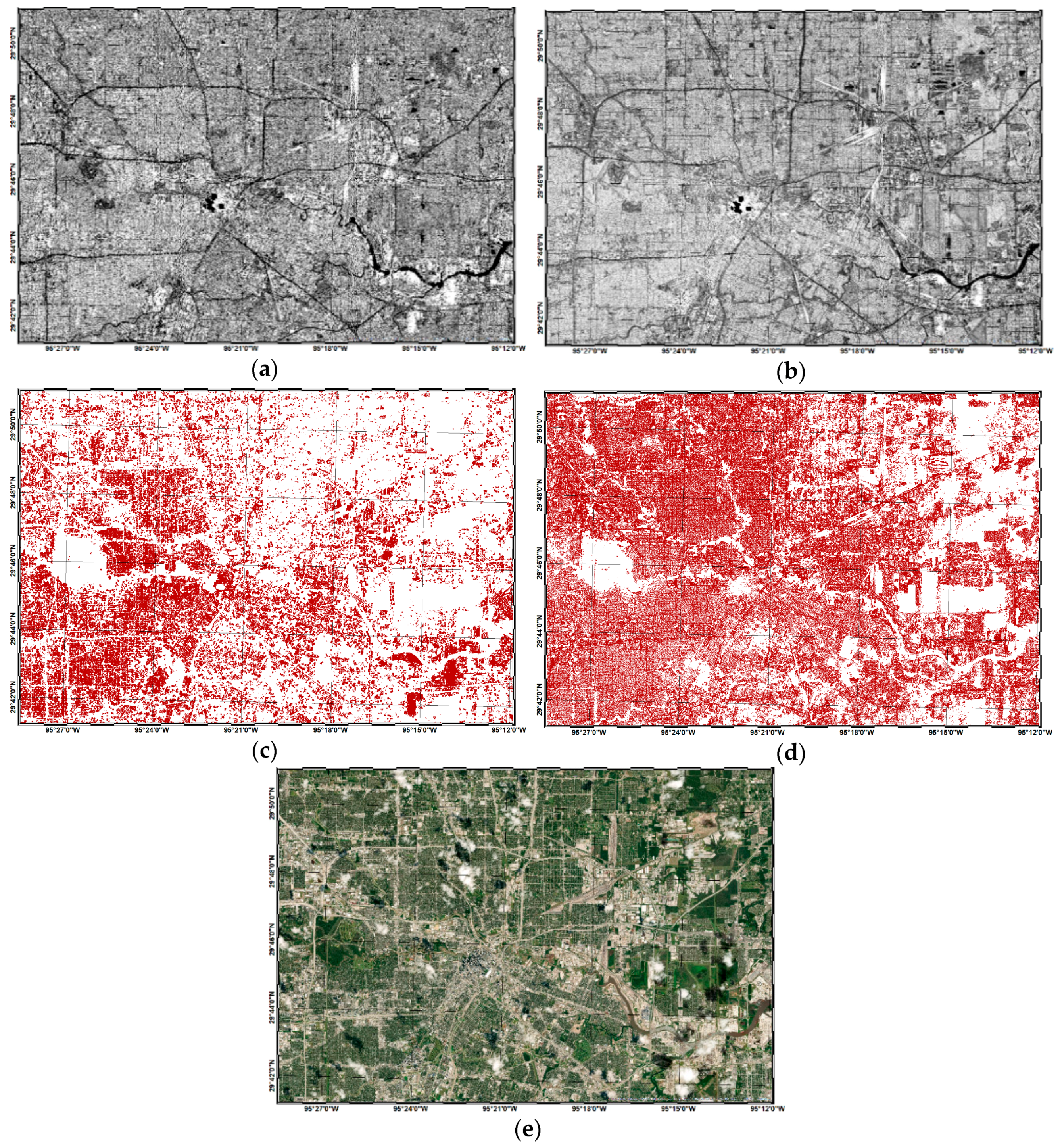
40], we obtained an S-1 building map at 5 and 20 m resolutions, depending on the S-1 operation mode considered. A sample of the product obtained is displayed in
Figure 3c,d. We notice that for both resolutions, the main built-up areas are delineated, although some differences are present due to the different spatial resolution. As shown in
Figure 3d, the map derived from SM contains more buildings, as its higher resolution also allows the detection of small houses. From
Figure 3e, it is possible to observe that the area is quite vegetated. This means that in a 20 m resolution pixel, the double-bounce contribution is mixed with that from the vegetation. This is an issue that needs to be taken into consideration in the evaluation of the final floodwater map.
To quantitatively analyze the resulting floodwater maps, we counted the number of pixels that were detected as flooded in bare soil areas, i.e., 2,910,880 and 43,533,877 in case of IW and SM images, respectively, and those added by the novel algorithm able to detect flooding in urban areas, which amounted to 322,147 and 1,687,048 pixels in the case of IW and SM acquisition, respectively. The affected areas increased by 11% (IW) and 4% (SM), which is quite relevant, especially if we consider that urban areas are the most sensitive in terms of risk and impact. The percentages are different because of the different spatial resolutions and, especially, the different spatial coverage (see
Figure 2).
In the following section, we present qualitative results for three case studies that were extracted from the data described above.
4.1. Test Case 1: Kingwood Area
The first case study contains an area in the north-west of Lake Houston. This includes the Kingwood area, where more than 3000 houses were damaged during Harvey [
47]. This area was imaged by S-1 with both acquisition modes, SM and IW. In
Figure 4a,b, we show the SAR intensity as a red, green and blue (RGB) composite of the reference (R) and flood (B = G) images. From this data set, we can clearly see (in red) all changes due to the flooding on bare soil, as the appearance of floodwater led to a decrease of the backscattering. We can also see some changes within built-up areas, which are depicted in cyan. The related backscatter increase is arguably caused by an increase in the double-bounce effect in areas where buildings are surrounded by water. However, since this effect is strongly dependent on the alignment of buildings with respect to the SAR flight line, its usage for identifying flooded buildings remains rather limited. To overcome this limitation and the ambiguity of the intensity signature, we make use of the information given by ρ.
Figure 4c,d illustrate the multi-temporal behavior of ρ over the same area, with an RGB composite (ρ
pre = R, ρ
co = B = G) layer. Focusing our analysis on the built-up areas, we notice a significant change in the ρ values for both IW and SM. Before the flooding occurs, ρ usually presents high values due to the temporal stability of buildings. However, in the event of floodwater appearance, this characteristic is no longer apparent and ρ drops off significantly, resulting in the condition ρ
pre > ρ
co, as depicted by areas in red color. Since other land classes, such as vegetation areas, exhibit similar behavior (note that red areas are spread all over the scene and have an overall big extension), the information given by ρ cannot be used in isolation to identify flooded buildings. For this reason, we make use of the building footprint presented in
Section 2.2. This layer is intersected with the areas that show a decrease of ρ to identify flooded buildings. The first case study contains an area to the north-west of the lake. The results obtained are given in
Figure 4g,h and depicted in dark blue. Most buildings, labeled as ‘flooded’ by the algorithm, are identified in both IW and SM images.
Figure 4e illustrates the Digital Globe VHR imagery along with the crowdsourcing points depicting damaged/flooded areas. The coherence-based algorithm detects most of the flooded buildings and appends them to the flooded bare soil areas identified by the initial step of the procedure (see
Figure 1). For example, this is the case of some houses located in the proximity of the lake border. As shown in the AOIs 2 and 3, in the areas containing many Digital Globe labels, our methodology detects a significant amount of flooded buildings. Moreover, the results of the proposed method present some additional flooded built-up areas with respect to crowdsourcing points. For instance, as depicted in AOI 1 from
Figure 4e, we notice that this area does not contain any Digital Globe labels. However, our method detects flooded buildings, as shown in AOI 1 from both IW and SM images (
Figure 4g,h). The latter are confirmed by aerial pictures taken over the respective areas on August 30, some examples being given in
Figure 5. The apparent misdetection of crowdsourcing is due to the fact that Digital Globe imagery was acquired 24 h after the S-1 IW image acquisition, and 36 h after the S-1 SM one. If we compare our results with damaged and affected built-up areas extracted from the FEMA inundation model (
Figure 4f), there is a good agreement between the two datasets. In particular, when looking at AOIs 1 and 2 in our maps (
Figure 4g,h) we notice that flooded buildings largely correspond to FEMA results from
Figure 4f. Moreover, as mentioned above, for AOI 1, the presence of floodwater is confirmed by aerial photos taken on August 30 (see
Figure 5).
4.2. Test Case 2: Industrial Area of Houston
The second case study is analogous to the one presented above. The area of interest is centered on an industrial area of Houston, where the chemical plant Arkema is located. The exact location of the chemical plant is highlighted on all maps shown in
Figure 6 by a blue square. Even though there are no crowdsourcing points available for this location, flooding by Hurricane Harvey is confirmed by aerial photos acquired over this area (
Figure 6f), as well as by information published on social media and official news outlets. From the SAR intensity information displayed in
Figure 6a,b, it is not possible to assess whether the chemical plant was flooded or not. The backscattering variations recorded in that specific area are not high enough to determine this. However, if we analyze the variations in ρ, an important drop-off is noticeable in both the IW and SM maps, as shown in
Figure 6c,d. This allows the delineation of a flooded area that comprises the chemical plant, as highlighted in dark blue in
Figure 6g,h. It is worth noting that flooded areas on bare soil are larger on the SM map than on the IW map. This is probably because the IW image was acquired 12 h after the SM image, when flooding had already receded. This is also confirmed by the GeoEye-1 images acquired the day after, where some flooded areas present on August 30 had already disappeared.
4.3. Test Case 3: Western Part of Houston
For the third case study, we focus on an area located in the western part of Houston that contains a very large number of damaged/flooded houses. According to the Digital Globe crowdsourcing data, more than 9000 houses were affected by the flood during Harvey. For this case, we considered only SAR data in IW mode, since the SM data with reduced swath do not cover this area. From the intensity images that are illustrated in
Figure 7a, we can see the impact of the flood both on bare soil areas depicted in red, as well as on urban areas depicted in cyan. To better characterize the latter, i.e., the flooded building class, we use the ρ information in the same manner as for the other case studies. In
Figure 7b, illustrating the ρ changes, we notice an important ρ
co drop-off, predominantly in the building areas that are surrounded by large bare soil areas that were classified as flooded. We can confidently hypothesize that the adjacent building areas are also prone to flooding. By merging these areas with the building footprint, we can detect the houses affected by the flood, as shown in
Figure 7e, in dark blue. These areas correspond to the Digital Globe crowdsourcing labels given in
Figure 7c. We also note that we detect another area in the lower left part of the map as flooded that was not covered by the Digital Globe data. If we compare our results of these additional areas with the FEMA model output, shown in
Figure 7d, we also observe a strong agreement in that area, thereby confirming the correctness of the algorithm’s outcome. The areas illustrating this aspect are depicted in the blue polygons in all the subfigures.
5. Discussion
The presence of water has been confirmed by an independent dataset in some of the urban areas mapped as flooded. To extend the analysis we further evaluate possible sources of errors of the proposed algorithm. For any procedure based on complex coherence, major errors are generally due to spatial and temporal decorrelations. The latter can be particularly critical for the case study analyzed in this paper because of the presence of vegetation within a cell and the possible occurrence of strong anthropic activities. Intense traffic conditions found in a big city such as Houston might, in theory, lead to false alarms because they potentially imply a decrease in the InSAR coherence. Even the presence of debris can cause decorrelation in an event such as that which occurred in Houston in 2017. To compare the effect of the aforementioned sources of decorrelation with the effect of the presence of floodwater, several ρ maps, with different temporal and spatial baselines, were extracted and their mean values for the urban areas classified, respectively, as Flooded (F) and Non-Flooded (NF), were computed. This analysis was carried out for the most challenging dataset, i.e., the IW images, with the lowest spatial resolution for which the presence of vegetation can play a predominant role. The ρ maps were computed considering four different configurations with respect to the flooded image (30 August 2017):
ρpre: both images were acquired before 30 August 2017.
ρpost: both images were acquired after 30 August 2017.
ρco: one image was acquired before 30 August 2017 (the closest one) and one during the event (30 August 2017).
ρcross: one image was acquired before and one after 30 August 2017. They were computed with same pre-event image as ρco, and with three post-event images acquired 6, 12 and 18 days after the flooded image (30 August 2017).
We averaged the above-mentioned ρ maps for F and NF classes to obtain eight different trends with respect to the perpendicular and temporal baseline, as summarized in
Figure 8.
From the graphs in
Figure 8, we notice that, as expected, the lowest coherence value is obtained for F ρ
co, where ρ reaches 0.25. This value is very close to that of open water (ρ
water = 0.1), which is generally considered a completely decorrelated class [
49]. Although ρ
co has the lowest temporal baseline, i.e., 6 days, from both graphs it is evident that F areas can be easily distinguished from the NF ones independently of the temporal and perpendicular baselines.
Looking at the two scatterplots in
Figure 8, it is clear that there is not any dependence of the InSAR coherence from the perpendicular baseline for the eight different classes, at least in the range of 0 to 90 m, while the temporal baseline is the one that affects the coherence the most, also in urban areas. From the scatterplot in
Figure 8a, it is evident that the maps not affected by floods with the highest temporal baselines have lower coherence values. It is worth considering that the residential areas containing vegetation and houses are usually small in size. Hence, in 20 m resolution pixels, although the double-bounce can be detected, the influence of other scattering mechanisms is also present. From
Figure 8a, it turns out that to better distinguish F from NF in urban areas, it is better to have a temporal baseline of 6 days, as this helps reduce all temporal decorrelation effects that are not related to the flood. This aspect becomes obvious when we look at the trends of ρ
pre for NF and F areas. Their values are different for higher temporal baselines, while no difference is noticeable for lower ones. It can be argued that this is due to the differences in the urban environment of the two classes.
The coherence maps with one month of temporal baseline were used to map double-bounce features and produce the built-up map. In this case, a higher temporal baseline is preferred for distinguishing buildings from vegetated areas, to highlight the decorrelation that is only due to vegetation.
The calculation of ρcross maps was done to check whether the potential presence of debris after such a catastrophic event can affect the coherence. As a result, the coherence slightly decreases to 0.42 in case of the urban F class but does not reach the value of 0.25 as is the case in the presence of water. In this latter case, it is worth considering that the temporal baseline is higher than 6 days of ρco, i.e., 12, 18 and 24 days, and the values are closer to those with a baseline of 30 days without crossing a catastrophic event. Thus, it is probably the temporal decorrelation due to the presence of vegetation between buildings that explains the drop-off. This type of land cover is rather common for Houston, where in the areas heavily affected by the flood, many small houses are surrounded by trees.
6. Conclusions
For the first time, a fully automatic algorithm capable of mapping floodwater in both rural and built-up areas using 20 m SAR data has been presented. It was designed to exploit the short temporal and perpendicular baselines of S-1 image pairs, thus taking advantage not only of SAR intensity, but also of InSAR coherence data. The algorithm was tested using the images acquired during the hurricane season in 2017, which caused large-scale flooding in and around the city of Houston (Texas). The floodwater maps obtained by applying the proposed SAR-based automatic floodwater mapping algorithm agree with those derived from a visual analysis of VHR optical images acquired shortly after the hurricane’s passage, when cloud cover no longer hampered their use. Moreover, a qualitative cross-comparison of our results with Digital Globe crowdsourcing points and the FEMA hydrological model has shown a strong agreement for most affected buildings.
An analysis of the S-1 image stack available revealed that a short temporal baseline of the co-event image pair is required to make the exploitation of coherence for flood detection effective. Conversely, a stack with longer temporal baseline is mostly suited to producing a prior classification of the built-up area. The range of perpendicular baselines ensured by the S-1 orbital tube does not affect the performance of the method.
The findings of this study demonstrate that the progress achieved in SAR imaging by the S-1 constellation (large spatial coverage, short revisit time, repeat-pass observations with small perpendicular baseline) potentially enabled emergency managers to fulfill their need for gathering NRT synoptic maps of the flood extent that also included urban settlements. The algorithm proposed can represent a valuable tool to pursue this objective. Nonetheless, further verifications of its performances considering other case studies are needed and are planned for the near future.
Moreover, advancing the capability to monitor floodwater within urban settlements paves the way for new applications to be developed in disaster risk management. For example, it becomes possible to regularly update/correct urban flood models through data assimilation procedures, as well as to estimate related variables such as river discharge and channel bathymetry. Different studies have already shown the value of satellite EO-derived floodwater extent maps for reducing the predictive uncertainty of numerical models and deriving key hydrological variables [
50,
51,
52]. However, the inability to delineate floodwater in urban areas has so far restricted such approaches to open areas, e.g., agricultural land outside the city centers.

 and
and 


