Clouds Classification from Sentinel-2 Imagery with Deep Residual Learning and Semantic Image Segmentation

Abstract

Detecting changes in land use and land cover (LULC) from space has long been the main goal of satellite remote sensing (RS), yet the existing and available algorithms for cloud classification are not reliable enough to attain this goal in an automated fashion. Clouds are very strong optical signals that dominate the results of change detection if they are not removed completely from imagery. As various architectures of deep learning (DL) have been proposed and advanced quickly, their potential in perceptual tasks has been widely accepted and successfully applied to many fields. A comprehensive survey of DL in RS has been reviewed, and the RS community has been suggested to be leading researchers in DL. Based on deep residual learning, semantic image segmentation, and the concept of atrous convolution, we propose a new DL architecture, named CloudNet, with an enhanced capability of feature extraction for classifying cloud and haze from Sentinel-2 imagery, with the intention of supporting automatic change detection in LULC. To ensure the quality of the training dataset, scene classification maps of Taiwan processed by Sen2cor were visually examined and edited, resulting in a total of 12,769 sub-images with a standard size of 224 × 224 pixels, cut from the Sen2cor-corrected images and compiled in a trainset. The data augmentation technique enabled CloudNet to have stable cirrus identification capability without extensive training data. Compared to the traditional method and other DL methods, CloudNet had higher accuracy in cloud and haze classification, as well as better performance in cirrus cloud recognition. CloudNet will be incorporated into the Open Access Satellite Image Service to facilitate change detection by using Sentinel-2 imagery on a regular and automatic basis.

1. Introduction

Detecting changes in land use and land cover (LULC) from space has long been the main goal of satellite remote sensing (RS) [1,2]. Although high-quality imagery opened from Landsat-8 and Sentinel-2 programs has provided an unprecedented source for satellite observation, various approaches and tools of change detection have been proposed and developed [3,4], and the potential of time series observations has also been demonstrated clearly [5,6], near real-time changes in LULC detected from spaceborne observations in a fully automated fashion are still not reliable. Clouds and their cast shadows found inevitably in an optical image are both very strong signals that represent a large fraction of changes by simply comparing two images. These unwelcome features suppress the real signal of surface changes and dominate the results of change detection if they are not removed completely from imagery. Clouds are some of the most common and dynamic features in satellite imagery of the earth’s surface, because approximately 52% of earth is covered by clouds at any moment [7], and land is covered by 0.10–0.15 fewer clouds than the oceans (i.e., land (41.5–45.0%) and ocean (55.0–56.5%)) [8]. A cloud can be defined as a mass of particles or droplets of dust, smoke, or steam, suspended in the atmosphere or existing in outer space [9]. It has various types and forms and has been receiving a lot of research interest in meteorology. For applications in RS, the classification of clouds is also a crucial step in the pre-processing of optical imagery [10]. The technology of object recognition advances very fast, and a lot of sound algorithms are available as well [11,12,13]. However, the general technology of object recognition is not suited for classifying clouds from RS imagery, because the exact boundaries of clustered particles and aerosols are usually very difficult to determine. As for cloud-cast shadows, Zhu et al. [14] have demonstrated that the view angle of a satellite sensor, the relative height of a cloud, as well as solar zenith and azimuth angles, can be used to generate corresponding shadow layers at quite a satisfying level, as long as the cloud layers are accurate. From the perspective of developing an automatic change detection system for LULC, therefore, the key task is to seek a reliable approach in classifying clouds first.

Generating a variety of thematic maps from satellite imagery has been approved and accepted as one of the major advantages of spaceborne observations back to the first introduction of the sensor Thematic Mapper in the Landsat-4 mission in 1982. Spectral, spatial, and radiometric resolutions kept being enhanced in the following Landsat missions, and also a lot of approaches were proposed to improve the accuracy of image classification, as reviewed by Zhu [15]. Apart from the classification of LULC, clouds and their cast shadows vary every minute and need to be masked out before any kind of RS activity is performed [10]. Zhu [15] also presented a comprehensive review of the works of cloud classification. He concluded that more time series-based cloud and cloud shadow classification algorithms are anticipated to emerge in consideration of the importance of accurate cloud and cloud shadow classification. To support the automatic processing of huge amounts of Landsat-8 data, a new algorithm called Fmask (Function of mask) was derived to identify clouds, shadows, snow, and water. Together with the combination of normalized temperature probability, spectral variability probability, and brightness probability, potential cloud pixels can be separated from clear-sky pixels with an accuracy as high as 96.4% [16]. To support the automatic processing of Sentinel-2 data, likewise, The European Space Agency (ESA) developed and released several free open source toolboxes, including Sen2cor, a processor for Sentinel-2 Level 2A product generation and formatting. Both Fmask and Sen2cor have pushed the general techniques of cloud classification to the limit, yet the current accuracy they can achieve is still insufficient to support the calculation of near real-time changes in LULC in a fully automated fashion.

Ball et al. [17] made a comprehensive survey of deep learning (DL) in RS and referred to previous approaches to image classification as shallow learning (SL) for contrast, such as the approaches of support vector machines, Gaussian mixtures models, hidden Markov models, and conditional random fields. They reviewed recent developments in theories, tools, and challenges that can be used in DL for RS and pointed out the advantage of a convolutional neural network (CNN) in many perceptual tasks. Since Krizhevsky et al. [18] accelerated operations in CNNs [19] using graphics processing unit (GPU) parallel computing, a vigorous growth in image classification using CNN architecture was triggered [20,21]. It started from general image classification and extended to the recognition of medical images and other fields of applications. Xie et al. [22] applied the excellent classification ability of CNNs to RS images for cloud classification and achieved quite a good recognition result. However, this CNN-based method was limited by the effect of clustering processing before CNN recognition. That is, cloud and cloud-free pixels might have been classified into the same group since the terrible clustering processing resulted in terrible cloud recognition results. While CNNs are widely employed in the field of image classification, another approach based on semantic images segmentation has also undergone tremendous changes due to the introduction of a fully convolutional neural network (FCN) in 2015 [23]. FCNs extended the ability of CNNs from entire image classifications to single-pixel identification. In other words, FCNs could label each pixel of the input image instead of only determining which group the input image belonged to. After that, the development of FCN-based architecture began to grow rapidly in the field of semantic images segmentation [24,25]. Zhan et al. [26] performed cloud classification tasks on Red-GreenBlue (RGB) images using FCN-based architecture. Drönner et al. [27] further extended FCN-based architecture to an architecture that could identify RS multispectral data. So far, the downsampling technique (pooling or striding) has been adopted in most FCN-based architecture to extract features. Although the technique has been proven to have the ability to capture deep texture features effectively, it has the disadvantage of losing the spatial information of the image [28]. However, we believe that in the field of RS, spatial information is more important than deep texture features. Compared to general image recognition tasks, the number of scenes in cloud classification applications is relatively small, so there is no need for too many deep texture features. In contrast, more spatial information is needed for training the model because thin and fractional clouds, which often appear at the boundaries of a normal cloud, are much more difficult to classify compared to the boundaries of objects from general image classification missions.

We propose an architecture called CloudNet, which was improved from the atrous spatial pyramid pooling (ASPP) module [29] and has good feature extraction performance for different resolution images. Residual learning [30] has improved the problem of gradient disappearance due to the increase in the number of layers in DL architecture. CloudNet incorporates residual learning to pass the spatial information of the upper layer to the next layer and prevents the loss of spatial information due to the increasing layers. The technique of downsampling (pooling or striding), used in CNNs and FCNs, was removed from CloudNet to keep the size of the input feature map in each layer consistent with the size of the output feature map. This design effectively avoided the loss of spatial information and achieved higher cirrus cloud recognition accuracy compared to existing methods. In the process of training CloudNet, we used the data augmentation technique [18] to generate 31,250 times more training materials than the original data for training. The process of generating manually labeled data was time-consuming and cost-inefficient. The technique allowed CloudNet to have stable cirrus identification capability without extensive training data. To our knowledge, the FCN-based architecture Deeplab v3+ [28] had the most outstanding performance in the field of semantic image segmentation in 2018. This study compared CloudNet to the classic method, scene classification (SCL) (produced by Sen2cor), and DL methods such as an FCN and Deeplab v3+. CloudNet had higher accuracy in cloud and haze classification than the other methods, and also had better performance in cirrus cloud recognition. It is worth mentioning that the number of training parameters in CloudNet was significantly smaller than in an FCN and Deeplab v3+, and thus the training time of CloudNet was less than the other two methods.

To summarize, a rigorous manually labeled Sentinel-2 cloud mask was released for a total of 5,017,600 pixels. The data augmentation technique allowed CloudNet to have stable cirrus identification capability without extensive training data. A novel DL architecture called CloudNet was proposed to pay more attention to spatial features than FCNs and Deeplab v3+ do, and thus it had better cirrus cloud classification performance than the other two methods. CloudNet is a flexible architecture that makes it easy to use any amount of spectral data as training material, and it is possible to map this method to other data from different satellites.

2. Training Dataset

Both the approaches of SL and DL for image classification require training, and the success of their application heavily relies on the quality and quantity of the training dataset. In the realm of RS, Ball [17] has pointed out that training data are usually expensive and error-prone, for they require some expert interpretation, large amounts of field work, and a long time to postprocess the data. They need to be representative and general enough to avoid overtraining as well. To develop a DL model of cloud classification, we started from some existing and available algorithms and attempted to generate the required dataset of clouds by ourselves.

CFMask is an algorithm that uses decision trees to prospectively label pixels in the scene and validate or discard those labels according to scene-wide statistics. CFMask is made available by the Earth Resources Observation and Science Center of the U.S. Geological Survey (USGS) in order to provide standard Landsat Level-1 data products, including cloud, cloud confidence, cloud shadow, and snow/ice masks. It has been incorporated into the L-8 Automatic Image Processing System to process all scenes of Landsat-8 imagery covering the Taiwan area on an operational basis [31]. However, CFMask has difficulties over bright targets, and thin clouds or haze are usually omitted. Figure 1 gives an example of the problems of standard Landsat Level-1 data products in cloud classification.

Sen2cor is an algorithm that combines several state-of-the-art techniques for performing atmospheric, terrain, and cirrus correction. Sen2cor can create bottom-of-atmosphere (BOA)-, terrain-, and cirrus-corrected reflectance images, aerosol optical thickness, water vapor, SCL maps, and quality indicators for cloud and snow probabilities [32]. Apart from official L2A products that are published on EO Browser and other Sentinel Hub services 48–60 h after L1C products are available, the Sen2cor tool can also be installed in our own server to process Level-2A data from L1C data directly. To process 10 granules covering the entirety of Taiwan, the time required for Level-2A data processing is approximately 20,800 s, using our personal computer based server. Like CFMask, the SCL maps of clouds also have difficulties over bright targets, and thin clouds and haze are usually omitted as well. Figure 2 gives an example of the problems of standard Sentinel-2 Level-2A data products in cloud classification.

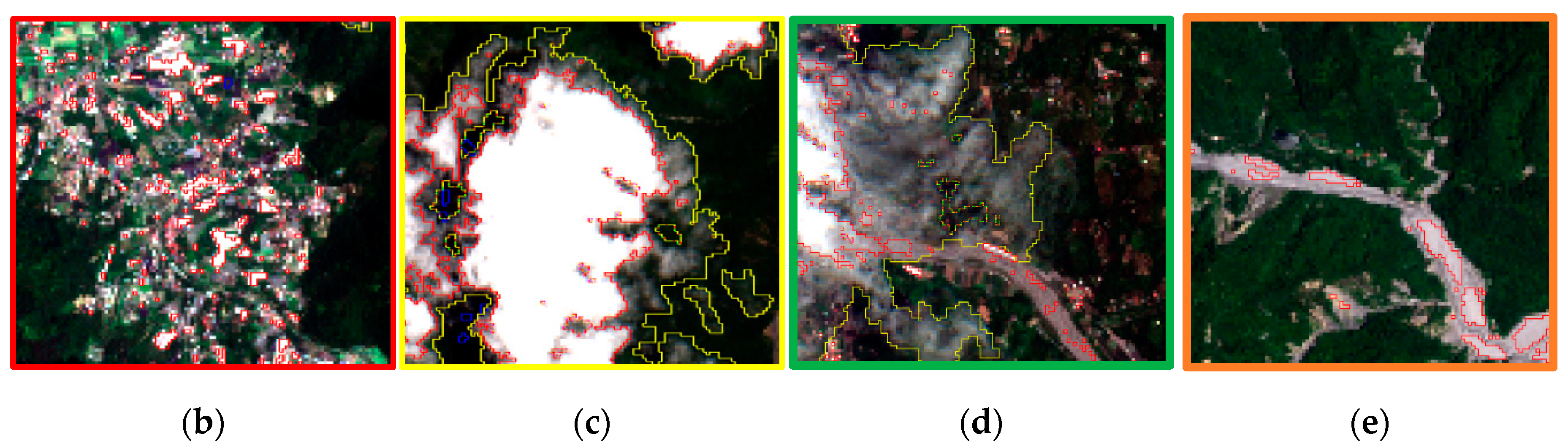
From the perspective of developing an automatic change detection system for LULC, the existing and available algorithms, such as CFMask and Sen2cor, are not accurate enough to generate the required dataset of clouds for training our DL model. Figure 3 gives an example of automatic change detection of LULC in Jianshi Township, Hsinchu County, Taiwan, overlaid over Sentinel-2 true color images (TCI) taken on (a) 9 August 2017 and (b) 14 August 2017, respectively. The red, blue, and yellow polygons were determined by the deviation automatically calculated from the SCL map, normalized difference vegetation index (NDVI), and normalized difference water index (NDWI). This gives an example for LULC studies where important information about change dynamics is impeded by clouds.

One alternative was to employ an operational cloud database, such as in the work by Drönner et al. [27], who used the well-validated Cloud Mask from the CLAAS-2 dataset [33]. However, that dataset was derived from geostationary Meteosat Spinning Enhanced Visible and Infrared Imager (SEVIRI) measurements for the time frame 2004–2015, which was not appropriate in training our DL model of cloud classification in terms of spatial, spectral, or temporal resolution. Another alternative was to mask all clouds manually in a certain number of Sentinel-2 images and prepare a detailed database of cloud and haze by ourselves, such as the work by Oreopoulos et al. [34], who used manual (visual) cloud masks developed at USGS for the collection of Landsat scenes. For two Sentinel-2 granules, the commercially available software Adobe Photoshop^® and ENVI^® were employed to determine and edit cloud masks in the level-1C product of a TCI, an enhanced RGB image composed of bands B04 (Red), B03 (Green), and B02 (Blue). To facilitate the training of DL, both the TCI and corresponding cloud masks were cut into a set of tiles with a uniform size of 224 × 224 pixels. A total of 100 tiles with 5,017,600 pixels were prepared in a week. This required a lot of labor, and the payback was a reliable database with high-quality data for training. Although the size and representativeness of the current training dataset were limited to these manually labeled tiles, they served as a reliable data source and a good start in developing and testing our new DL architecture. The training dataset of all TCIs and corresponding cloud masks, including a total of 100 tiles with a uniform size of 224 × 224 pixels, are available in the Supplementary Materials.

3. Architecture and Experimental Setup

To evaluate the performance of various DL architectures in cloud classification and to gain a better understanding of the mechanism behind improving accuracy, we followed the literature to set up the three most popular DL architectures in perceptual tasks, including a CNN, an FCN, and Deeplab v3+. Based on the acquired experience, a novel DL architecture, CloudNet, was proposed and investigated.

3.1. CNNs

The standard CNN architecture is comprised of input, hidden, and output layers. The input layer is an interface for digesting training data, while the output layer is an interface for exporting model prediction. The hidden layers in between mainly contain the convolutional layers, the pooling layers, and the fully connected layers. A convolutional layer is made up of many filters for extracting features from input images. The exact features to be extracted by these filters are not pre-defined, but instead, they are gradually learned through the process of training. During the training iteration, each filter acts more and more like an independent feature extractor that captures a particular feature until the training process is completed. All captured features are integrated as a feature map. The pooling layer is then used to refine some more representative features from this feature map. As a consequence, the size of the feature map is not only reduced (usually to half of the input length and width), but the training process is also accelerated. The fully connected layer is made up of one-dimensional nodes. The links among nodes in different layers are the weighting parameters to be trained. As they are similar to the filters in the convolutional layer, each trainable weighting parameter gradually approaches a certain value as the training progresses. In general, the hidden layer is a combination of convolutional layers and pooling layers, and a number of repetitions of the combination and a number of filters per convolutional layer vary depending on the architecture design. The hidden layer is often ended with some fully connected layers that export the predicted results to the output layers. The processing and downsampling of the feature map among layers in a CNN architecture are illustrated in Figure 4. In the first five layers (the convolutional and pooling layers), various downsampling techniques (pooling or striding) are applied to gradually reduce the length and width of the feature map to obtain deep texture features. In the last three layers (fully connected layers), a 2-D feature map with multichannels is converted into a 1-D vector and exported to a 1-D model prediction.

3.2. FCN

Based on CNN architecture, FCN architecture replaces the fully connected layer (the last part in the hidden layer) with a fully convolutional layer. As a result, the predicted results from an FCN retain a 2-D feature map and achieve pixel-level prediction, which is superior to the 1-D prediction from a CNN. Furthermore, a FCN speeds up the entire model training process by significantly reducing the number of trainable parameters, compared to the number required by a CNN. The processing and downsampling of the feature map among layers in FCN architecture is illustrated in Figure 5. Note that the last three layers of the fully connected layers of the CNN shown in Figure 4 are replaced by three fully convolutional layers in our FCN architecture for cloud classification. The predicted 2-D feature map is also upsampled to fit the size of the input image.

3.3. Deeplab v3+

Deeplab is a DL model for semantic image segmentation dedicated to assigning semantic labels to every pixel in the input image [35]. Its latest version, Deeplab v3+, is now open source and fully supported by Google. The hidden layer of Deeplab v3+ is divided into two parts: (1) The feature extraction part is based on improved Xception architecture [36], which is an FCN-based architecture; and (2) the upsampling part is based on the output of improved Xception architecture followed by the ASPP module, which is made up of SPP [37] and atrous convolution [35]. ASPP architecture has proven to be good for robustly segmenting objects at multiple scales [29]. Deeplab v3+ applies the ASPP technique to improve its ability to identify the same objects with different sizes in the image. At the stage of restoring the feature map back to the size of the original input image, Deeplab v3+ combines a shallow feature map with a deep feature map to recover lost boundary information. Finally, the feature map is restored to the same size as the input layer image by applying the upsampling technique. The processing and downsampling of the feature map among layers in Deeplab v3+ architecture are illustrated in Figure 6. FCN-based Xception architecture is used to capture deep texture features. In ASPP architecture, three convolutional layers with different atrous rates and one average pooling layer are applied to create four different feature maps. These feature maps are then concatenated to one feature map. The feature map generated by ASPP is first upsampled and then concatenated with the feature from the shallow layer of Xception. The upsampling technique is applied in the last layer of Deeplab v3+ to resize the 2-D feature map to fit the size of the input image and get the 2-D prediction results.

3.4. CloudNet

After setting up the CNN, FCN, and Deeplab v3+ architectures for cloud classification, we proposed the CloudNet architecture with residual learning and semantic image segmentation. The ASPP architecture in Deeplab v3+ was kept in CloudNet for feature extraction. By increasing the number of branches and the atrous rate, CloudNet is able to increase the size of the field of view to capture more features, as well as to recognize clouds at different sizes. Meanwhile, CloudNet employs residual learning to preserve spatial information of a specific layer and pass it to the next layer. Note that unlike the feature map for restoring spatial information in Deeplab v3+, which is four times smaller than the input image, CloudNet delivers full-size image spatial information in each layer. The general structure for feature extraction in the deep convolution network (Xception in Deeplab v3+) usually performs multiple downsampling operations to obtain deep texture information. In contrast, CloudNet is able to preserve spatial information, for it does not apply any downsampling operation. The output feature map in each layer in CloudNet is the same size as the original input image, which indicates that the upsampling technique in the FCN is not required, and pixel-level recognition and classification can still be achieved. Another merit of CloudNet is adding full image information (residual) from the upper layer at the end of each layer. This keeps CloudNet from losing spatial information after increasing the number of layers. Since most RS imagery is acquired with multispectral bands, CloudNet was designed to be trained with different combinations of spectral bands. The processing and downsampling of the feature map among layers in the CloudNet architecture are illustrated in Figure 7. Note that the architecture within the blue dotted line is a single training unit for CloudNet.

Figure 8 illustrates the training unit of CloudNet, which is shown as a blue dotted line in Figure 7. In the figure, (1 × 1 conv, 4) represents a convolutional layer with only 1 convolutional node, where the number of channels is 4. It was used to normalize the number of channels of the feature map delivered from the previous layer, to avoid the number of channels of the feature map from increasing infinitely as the number of layer increased. In the figure, (3 × 3 conv, 4 rate = 2) represents a convolutional layer with a matrix of 3 convolutional nodes in length and width, where the number of channels is 4 and the distance between two convolutional nodes is 2 pixels (as shown in the image with the orange square). By increasing the value of the atrous rate, the convolutional layer could obtain a larger field of view. Likewise, the full image information (residual) from the upper layer was added back to avoid the loss of spatial information due to the increasing number of layers.

4. Evaluation

The performance of DL is highly dependent on the configuration of hardware and software. In this research, CloudNet was trained by an ordinary personal computer equipped with a Central Processing Unitof Intel’s i7 4790 and a GPU of NVIDIA’s GTX 1080Ti packed with 11 Gbps GDDR5X memory. The operating system was Windows 10, and the DL algorithm was implemented by Python (version: 3.1.6) language with the Keras library (version: 2.1.6), a wrapper library for Tensorflow (version: 1.6.0).

A large amount of data is usually needed for training a DL model. For cases with an insufficient amount of training data, such as in our manual (visual) cloud masks, a couple of practical techniques of data augmentation can be employed to generate a large amount of training data [18]. First, we used a 224 × 224 pixel window with a step size of 18 pixels to expand the original training data (2240 × 2240 pixels), resulting in a total of 12,769 images with partially overlapped pixels. A total of 2769 images were selected from the training set and reserved as validation data, while the remaining 10,000 sub-images were used as a training set. Second, the training data in each iteration was processed by different operations in a total of 250 training iterations, including horizontal flip (50% probability), vertical flip (50% probability), rotation (angle between −10 and +10 degrees), zooming (magnification from 1.1 to 1.4 times), and cropping (in the training image with a size of 224 × 224 pixels, a matrix of 200 × 200 pixels was randomly selected).

The training process was equivalent to the exploration of the minimum value on the plane of a loss function. We used a stochastic gradient descent with momentum for backpropagation. It was like putting a momentum ball on the plane of a loss function, and the ball would follow the gradient direction. In each training iteration, the ball would slowly adjust its direction until the lowest point of the plane was reached, which meant the training was completed. The total number of epochs was set to 250, the batch size was set to 16 samples, the momentum value was set to 0.95, the weight decay value was set to 0.00005, and the learning rate was described as

$$\mathrm{learning}\mathrm{rate}=0.01\ast {\left(1-\frac{\mathrm{epoch}}{250}\right)}^{0.9}.$$

(1)

Note that these parameters were basically set as those values suggested by the work of Long et al. [23]. Only a slight adjustment was introduced.

The following indicators were calculated to evaluate the performance of the segmentation in the test dataset with the model constructed in this study. These indicators may be useful in illustrating the context in which this method can apply. True positive (TP) indicates the number of cloud pixels that were predicted correctly. False positive (FP) means the number of the predicted cloud pixels that were incorrect. False negative (FN) is the number of cloud pixels that were not classified. True negative (TN) indicates the number of non-cloud pixels that were classified correctly. P represents the actual number of pixels in the cloud (TP + FN). N represents the number of pixels (FP + TN) that were not actually clouds.

The following indicators suggested from the literature were calculated to evaluate the performance of the segmentation in the test dataset with the model constructed in this study: (1) true positive rate (TPR) indicates the proportion of TPs to positives; (2) true negative rate (TNR) indicates the proportion of TNs to negatives; (3) precision represents the proportion of TPs in all pixels that were predicted to be clouds (TP + FP); (4) pixel accuracy indicates the proportion of the correct pixel count (TP + TN) in all pixels (P + N); (5) intersection over union (IoU or IU) indicates the proportion of the intersection of P and G in the union of P and G (note that P stands for the prediction results, and G stands for the ground truth), and all of the above indicators have been used in image segmentation studies [23,25,28,35]; (6) IoU (cloud) indicates the proportion of TP in (TP + FP + FN); (7) IoU (cloud-free) indicates the proportion of TN in (TN + FP + FN); (8) mIoU represents the average of IoU (cloud) and IoU (cloud-free); and (9) kappa is an evaluation standard that was used to compare the accuracies between model and random classifiers and was generally more representative in evaluating model than accuracy [38].

5. Results

To evaluate the performance of various DL architectures in classifying clouds, standard Sentinel-2 Level-2A data products taken on 16 May 2018 covering granules T51QUG and T51QTG were selected. The union of their corresponding SCL map of thin clouds (class 10), high-probability clouds (class 9), and medium-probability clouds (class 8), was regarded as the SCL cloud mask. As aforementioned, manual (visual) cloud masks were used as the benchmark. The true color composite of BOA reflectance at bands B04 (Red), B03 (Green), and B02 (Blue) was used as the input image. The predicted cloud masks from FCN, Deeplab v3+, and CloudNet were compared to the benchmark of cloud masks, and a total of eight indicators are listed in

Table 1. Evaluation of various deep learning (DL) architectures in classifying clouds, using eight indicators. TPR: True positive rate; TNR: True negative rate; IoU: Intersection over union; mIoU: The average of IoU (cloud) and IoU (cloud-free).

Method	SCL	FCN	Deeplab v3+	CloudNet
TPR (cloud)	0.8646	0.9429	0.9544	0.9630
TNR (cloud-free)	0.9812	0.9032	0.9230	0.9446
Precision	0.9934	0.9696	0.9810	0.9827
IoU (cloud)	85.96%	91.59%	92.61%	94.70%
IoU (cloud-free)	67.95%	76.08%	79.27%	84.24%
mIoU	76.96%	83.83%	85.51%	89.47%
Kappa	0.8713	0.8204	0.8486	0.8873
Pixel accuracy	89.18%	93.36%	94.51%	95.87%

. The results indicate that CloudNet surpassed an FCN, Deeplab v3+, and an SCL for all indicators: TPR (cloud), TNR (cloud-free), precision, IoU (cloud), IoU (cloud-free), mIoU, kappa, and pixel accuracy. The accuracy of CloudNet was slightly less than the SCL only in terms of two exceptions: TNR (cloud-free) and precision, yet its overall precision (95.87%) was significantly higher than the SCL (89.18%). In other words, a slight sacrifice in CloudNet’s sensitivity to cloud-free pixels could further enhance its capability for classifying clouds. This is related to the designed architecture of CloudNet. Its capability to capture a deeper feature map would be weakened after removing the layers of downsampling. However, we could increase CloudNet’s receptive field by increasing its number of branches and hence compensate for the influence of removing downsampling layers.

To gain a better understanding of the pros and cons of each method in cloud classification, we present eight regions with different types and forms of a cloud as eight RGB images, as shown in the first row of

Table 2. Optimization of the number of layers to be used by CloudNet.

Layers	4	6	8	10	12	14
Predict time (20 scenes)	9.469 s	13.215 s	16.798 s	20.220 s	24.509 s	39.459 s
TPR (cloud)	0.9655	0.9616	0.9630	0.9648	0.9694	0.5645
TNR (cloud-free)	0.9440	0.9489	0.9446	0.9450	0.9396	0.9683
Precision	0.9826	0.9841	0.9827	0.9829	0.9813	0.9832
IoU (cloud)	94.93%	94.69%	94.70%	94.88%	95.19%	55.91%
IoU (cloud-free)	84.80%	84.28%	84.24%	84.71%	85.39	39.89%
mIoU	89.86%	89.48%	89.47%	89.80%	90.29%	47.90%
Kappa	0.8917	0.8875	0.8873	0.8910	0.8965	0.3588
Pixel accuracy	96.04%	95.86%	95.87%	96.01%	96.24%	65.89%

. The predicted cloud mask of each region from SCL, FCN, Deeplab v3+, and CloudNet are shown from rows 2 to 5. Apparently, the SCL failed to classify many cirrus cloud pixels, while the FCN successfully detected most cloud pixels in spite of its poor performance near the edge of clouds. Due to the process of downsampling, the FCN lost some details of images inevitably. Take column 3 in Figure 9 as an example: The FCN (row 3) indeed captured more cloud pixels than the SCL (row 2) did. However, the FCN was only capable of depicting the boundary approximately, yet was incapable of delineating the details of cloud masks. The performance of Deeplab v3+ near the edge of clouds was better than the FCN’s, but it was difficult for Deeplab v3+ to identify those cases with more fractional clouds. Though there is a mechanism to retain spatial information (residual learning), some spatial information was still inevitably lost during the process of downsampling. For the cases of thin clouds (columns 5 and 6), CloudNet performed better than Deeplab v3+ in identifying those thin clouds in the middle. For the cases of clouds over bright objects (columns 8), a lot of misclassifications (houses and riverbeds) were found in the SCL, yet every DL model did a good job.

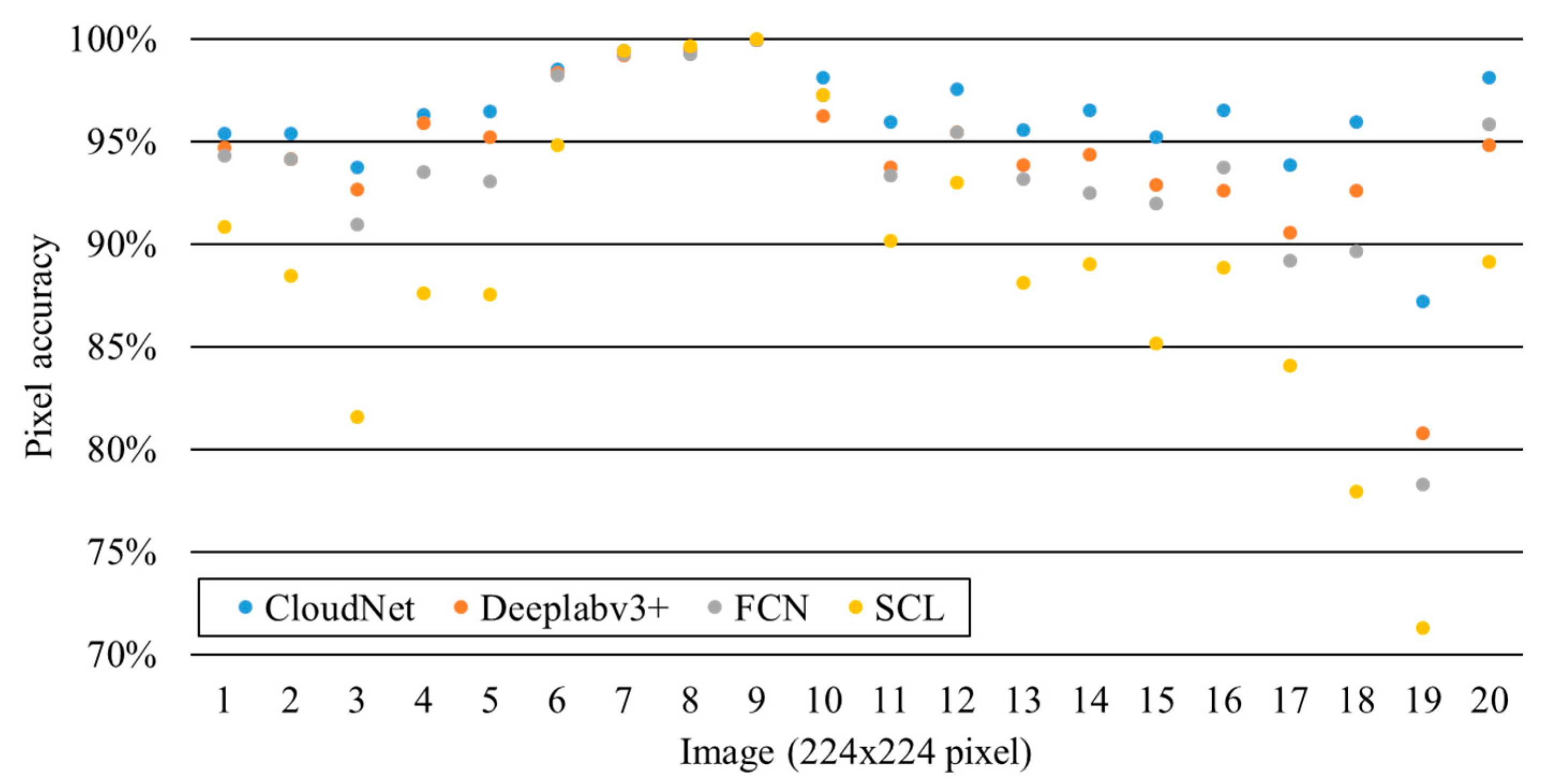
By repeating the same calculation of eight indicators for all 20 scenes (1,003,520 pixels in total), the results of pixel accuracy obtained from the SCL, the FCN, Deeplab v3+, and CloudNet are plotted in Figure 10 for comparison. CloudNet was indeed capable of identifying most of the cloud pixels and achieved the highest pixel accuracy for all 20 scenes. The overall performance of the SCL, in contrast, was the worst among the four methods. In the scenes with fewer cirrus clouds (scenes 7 and 9), the performance of the SCL was nearly the same as the other methods. In the scenes with more cirrus cloud (scenes 6, 18, and 19), the merit of CloudNet in classifying clouds was apparent.

Another important evaluation of DL architecture is the required time for cloud classification, which is closely related to the number of parameters to be determined. General DL architecture, such as in an FCN, often requires a large number of filters to capture many features. For applications in cloud classification, however, the scene is not that complex, so the number of filters in CloudNet could be largely reduced to only 28 filters in each layer, compared to the FCN and Deeplab v3+, which often need more than 1000 filters in each layer. Excessive parameters not only require a huge amount of GPU memory, but also cost a lot of time to calculate. Take one image with 224 × 224 pixels as an example: The number of parameters and the time for cloud classification required by the FCN, Deeplab v3+, and CloudNet are compared in Figure 11. The FCN had the largest number of parameters and the longest time for cloud detection, followed by Deeplab v3+, and then CloudNet.

6. Discussion

To meet the requirements for change detection from Sentinel-2 imagery on a regular and automatic basis in the future, we also conducted a few numerical experiments, with the intention of determining the optimized number of branches and layers to be used by CloudNet. The results shown in Table 2 indicate that as the number of layers increased, the pixel accuracy increased accordingly and reached a peak value at a number of 12 layers, which suggests the optimized number of layers to be used in CloudNet is 12 layers. Note that when CloudNet was set to 6 layers, two indicators (TNR and precision) were the highest. This can be regarded as the benchmark for CloudNet for this scene, similar to the SCL, since the SCL also had the best results in the evaluation metrics of TNR and precision.

The results shown in

Table 3. Optimization of the number of branches to be used by CloudNet.

Branches	4	6	8	10
Predict time (20 scenes)	12.496 s	25.587 s	24.509 s	41.950 s
TPR (cloud)	0.9648	0.9572	0.9694	0.9667
TNR (cloud-free)	0.9423	0.9569	0.9396	0.9189
Precision	0.9821	0.9865	0.9813	0.9750
IoU (cloud)	94.81%	94.48%	95.19%	94.33%
IoU (cloud-free)	84.49%	83.92%	85.39%	82.84%
mIoU	89.65%	89.20%	90.29%	88.59%
Kappa	0.8893	0.8843	0.8965	0.8777
Pixel accuracy	95.96%	95.71%	96.24%	95.55%

indicate that as the number of branches increased, the pixel accuracy increased accordingly and reached a peak value at a number of 8 branches, which suggests the optimized number of branches to be used in CloudNet is 8 branches. To summarize, after optimizing the number of layers and branches, CloudNet performed the best under the architecture of 12 layers and 8 branches. Pixel accuracy reached 96.24%, and kappa was approximately 0.9.

The uniqueness in this paper for advancement of cloud classification methods is CloudNet, a new DL architecture with an enhanced capability of feature extraction for classifying clouds. This was achieved by employing parallel convolution layers for deep feature extraction, instead of the general practice of the downsampling technique adopted in most FCN-based architectures to extract features. A significant amount of GPU memory consumption was supposed to be the price that CloudNet had to pay. However, we conducted a sensitivity test and realized that the number of filters in each layer of CloudNet could be reduced from more than 1000 to only 28 without losing accuracy. This is attributed to the fact that clouds are not as complicated as other objects. Once the deep feature is extracted and the cloud boundary is retained, there is not much to differentiate in the cloud itself. In other words, CloudNet uses fewer amounts of filters to achieve the same or even higher cloud recognition capability, compared to a general deep learning model with more than 1000 filters in most layers. Another novel design of CloudNet is that the full spatial information in each layer is passed by the method described in Reference [30], rather than the general method of ASPP that involves pooling. As a result, more spatial information is retained by CloudNet.

7. Conclusions

To support the automatic change detection of LULC from Sentinel-2 imagery, we propose a new DL architecture, namely CloudNet, with an enhanced capability of feature extraction for classifying clouds. CloudNet incorporates residual learning to pass spatial information and prevents the loss of spatial information due to increasing layers. The technique of downsampling (pooling or striding) is removed from CloudNet to keep the size of the input feature map in each layer consistent with the size of the output feature map. This design effectively avoided the loss of spatial information and achieved higher cirrus cloud recognition accuracy compared to existing methods. In the process of training CloudNet, the data augmentation technique was used to generate 31,250 times more training material than the original data for training. This study compared CloudNet to the traditional method of SCL and DL methods, including an FCN and Deeplab v3+. CloudNet had higher accuracy in cloud and haze classification than other methods, and also had better performance in cirrus cloud recognition. We could easily observe through visual experiments that the prediction of CloudNet in cirrus clouds was significantly better than other methods. We also demonstrated that CloudNet improved the accuracy of predictions without causing performance degradation and other costs. CloudNet will be incorporated into the Open Access Satellite Image Service (OASIS, http://oasis.ncku.edu.tw) [31] to support the calculation of near real-time changes in LULC over the Taiwan area in a fully automated fashion. A total of 5,017,600 pixels (manually labeled Sentinel-2 clouds) were created for training and validation in this study, and we released the manually labeled cirrus-sufficient dataset so that researchers in related fields can effectively apply it to their own research. Although the size and representativeness of the current training dataset are limited to these manually labeled tiles, they served as a reliable data source and a good start in developing and testing our new DL architecture. The future work that is planned is employing an export system [39] to facilitate the preparation of cloud masks from the results of change detection from the time series of consecutive Sentinel-2 images, as well as adding physical characteristics of clouds and/or satellite images to derive cloud masks. This new DL architecture can also be modified to classify other LULC classes, such as landslides and shadows. The long-term (12 years) and detailed (2-m resolution) landslide inventory of Taiwan [39] would be an ideal data source for training and testing our new DL architecture in classifying landslides.

References

1. Singh, A. Review article digital change detection techniques using remotely-sensed data. Int. J. Remote Sens. 1989, 10, 989–1003. [Google Scholar] [CrossRef]
2. Green, K.; Kempka, D.; Lackey, L. Using remote sensing to detect and monitor land-cover and land-use change. Photogramm. Eng. Remote Sens. 1994, 60, 331–337. [Google Scholar]
3. Mas, J.-F. Monitoring land-cover changes: A comparison of change detection techniques. Int. J. Remote Sens. 1999, 20, 139–152. [Google Scholar] [CrossRef]
4. Lambin, E.F.; Strahlers, A.H. Change-vector analysis in multitemporal space: A tool to detect and categorize land-cover change processes using high temporal-resolution satellite data. Remote Sens. Environ. 1994, 48, 231–244. [Google Scholar] [CrossRef]
5. Yang, X.; Lo, C. Using a time series of satellite imagery to detect land use and land cover changes in the atlanta, georgia metropolitan area. Int. J. Remote Sens. 2002, 23, 1775–1798. [Google Scholar] [CrossRef]
6. Lunetta, R.S.; Knight, J.F.; Ediriwickrema, J.; Lyon, J.G.; Worthy, L.D. Land-cover change detection using multi-temporal modis ndvi data. Remote Sens. Environ. 2006, 105, 142–154. [Google Scholar] [CrossRef]
7. Downs, R.M.; Day, F.A. National Geographic Almanac of Geography; National Geographic Society: Washington, DC, USA, 2005. [Google Scholar]
8. Stubenrauch, C.; Rossow, W.; Kinne, S.; Ackerman, S.; Cesana, G.; Chepfer, H.; Di Girolamo, L.; Getzewich, B.; Guignard, A.; Heidinger, A. Assessment of global cloud datasets from satellites: Project and database initiated by the gewex radiation panel. Bull. Am. Meteorol. Soc. 2013, 94, 1031–1049. [Google Scholar] [CrossRef]
9. Mallinson, J.V. The american heritage student science dictionary. Sci. Act. 2006, 43, 47. [Google Scholar]
10. Hollstein, A.; Segl, K.; Guanter, L.; Brell, M.; Enesco, M. Ready-to-use methods for the detection of clouds, cirrus, snow, shadow, water and clear sky pixels in sentinel-2 msi images. Remote Sens. 2016, 8, 666. [Google Scholar] [CrossRef]
11. Pal, N.R.; Pal, S.K. A review on image segmentation techniques. Pattern Recognit. 1993, 26, 1277–1294. [Google Scholar] [CrossRef]
12. Durand, N.; Derivaux, S.; Forestier, G.; Wemmert, C.; Gançarski, P.; Boussaid, O.; Puissant, A. Ontology-based object recognition for remote sensing image interpretation. In Proceedings of the 19th IEEE International Conference on Tools with Artificial Intelligence, ICTAI 2007, Patras, Greece, 29–31 October 2007; pp. 472–479. [Google Scholar]
13. Hau, C.C. Handbook of Pattern Recognition and Computer Vision; World Scientific: London, UK, 2015. [Google Scholar]
14. Zhu, Z.; Wang, S.; Woodcock, C.E. Improvement and expansion of the fmask algorithm: Cloud, cloud shadow, and snow detection for landsats 4–7, 8, and sentinel 2 images. Remote Sens. Environ. 2015, 159, 269–277. [Google Scholar] [CrossRef]
15. Zhu, Z. Change detection using landsat time series: A review of frequencies, preprocessing, algorithms, and applications. Isprs J. Photogramm. Remote Sens. 2017, 130, 370–384. [Google Scholar] [CrossRef]
16. Zhu, Z.; Woodcock, C.E. Object-based cloud and cloud shadow detection in landsat imagery. Remote Sens. Environ. 2012, 118, 83–94. [Google Scholar] [CrossRef]
17. Ball, J.E.; Anderson, D.T.; Chan, C.S. Comprehensive survey of deep learning in remote sensing: theories, tools, and challenges for the community. J. Appl. Remote Sens. 2017, 11, 042609. [Google Scholar]
18. Krizhevsky, A.; Sutskever, I.; Hinton, G.E. Imagenet classification with deep convolutional neural networks. In Proceedings of the 25th International Conference on Neural Information Processing Systems—Volume 1; Curran Associates Inc.: Lake Tahoe, Nevada, 2012; pp. 1097–1105. [Google Scholar]
19. LeCun, Y.; Boser, B.; Denker, J.S.; Henderson, D.; Howard, R.E.; Hubbard, W.; Jackel, L.D. Backpropagation applied to handwritten zip code recognition. Neural Comput. 1989, 1, 541–551. [Google Scholar] [CrossRef]
20. Zeiler, M.D.; Fergus, R. Visualizing and understanding convolutional networks. arXiv, 2013; arXiv:1311.2901. [Google Scholar]
21. Simonyan, K.; Zisserman, A. Very deep convolutional networks for large-scale image recognition. arXiv, 2014; arXiv:1409.1556. [Google Scholar]
22. Xie, F.; Shi, M.; Shi, Z.; Yin, J.; Zhao, D. Multilevel cloud detection in remote sensing images based on deep learning. Ieee J. Sel. Top. Appl. Earth Obs. Remote Sens. 2017, 10, 3631–3640. [Google Scholar] [CrossRef]
23. Long, J.; Shelhamer, E.; Darrell, T. Fully convolutional networks for semantic segmentation. arXiv, 2014; arXiv:1411.4038. [Google Scholar]
24. Huang, G.; Liu, Z.; van der Maaten, L.; Weinberger, K.Q. Densely connected convolutional networks. arXiv, 2016; arXiv:1608.06993. [Google Scholar]
25. Ronneberger, O.; Fischer, P.; Brox, T. U-net: Convolutional networks for biomedical image segmentation. arXiv, 2015; arXiv:1505.04597. [Google Scholar]
26. Zhan, Y.; Wang, J.; Shi, J.; Cheng, G.; Yao, L.; Sun, W. Distinguishing cloud and snow in satellite images via deep convolutional network. IEEE Geosci. Remote Sens. Lett. 2017, 14, 1785–1789. [Google Scholar] [CrossRef]
27. Drönner, J.; Korfhage, N.; Egli, S.; Mühling, M.; Thies, B.; Bendix, J.; Freisleben, B.; Seeger, B. Fast cloud segmentation using convolutional neural networks. Remote Sens. 2018, 10, 1782. [Google Scholar] [CrossRef]
28. Chen, L.-C.; Zhu, Y.; Papandreou, G.; Schroff, F.; Adam, H. Encoder-decoder with atrous separable convolution for semantic image segmentation. arXiv, 2018; arXiv:1802.02611. [Google Scholar]
29. Chen, L.-C.; Papandreou, G.; Schroff, F.; Adam, H. Rethinking atrous convolution for semantic image segmentation. arXiv, 2017; arXiv:1706.05587. [Google Scholar]
30. He, K.; Zhang, X.; Ren, S.; Sun, J. Deep residual learning for image recognition. arXiv, 2015; arXiv:1512.03385. [Google Scholar]
31. Liu, C.-C.; Nakamura, R.; Ko, M.-H.; Matsuo, T.; Kato, S.; Yin, H.-Y.; Huang, C.-S. Near real-time browsable landsat-8 imagery. Remote Sens. 2017, 9, 79. [Google Scholar] [CrossRef]
32. Müller-Wilm, U. Sen2cor Configuration and User Manual; Telespazio VEGA Deutschland GmbH: Darmstadt, Germany, 2016. [Google Scholar]
33. Benas, N.; Finkensieper, S.; Stengel, M.; van Zadelhoff, G.J.; Hanschmann, T.; Hollmann, R.; Meirink, J.F. The msg-seviri-based cloud property data record claas-2. Earth Syst. Sci. Data 2017, 9, 415–434. [Google Scholar] [CrossRef]
34. Oreopoulos, L.; Wilson, M.J.; Várnai, T. Implementation on landsat data of a simple cloud-mask algorithm developed for modis land bands. IEEE Geosci. Remote Sens. Lett. 2011, 8, 597–601. [Google Scholar] [CrossRef]
35. Chen, L.-C.; Papandreou, G.; Kokkinos, I.; Murphy, K.; Yuille, A.L. Deeplab: Semantic image segmentation with deep convolutional nets, atrous convolution, and fully connected crfs. arXiv, 2016; arXiv:1606.00915. [Google Scholar]
36. Chollet, F. Xception: Deep learning with depthwise separable convolutions. arXiv, 2016; arXiv:1610.02357. [Google Scholar]
37. He, K.; Zhang, X.; Ren, S.; Sun, J. Spatial pyramid pooling in deep convolutional networks for visual recognition. arXiv, 2014; arXiv:1406.4729. [Google Scholar]
38. Cohen, J. A coefficient of agreement for nominal scales. Educ. Psychol. Meas. 1960, 20, 37–46. [Google Scholar] [CrossRef]
39. Liu, C.-C. Preparing a landslide and shadow inventory map from high-spatial-resolution imagery facilitated by an expert system. J. Appl. Remote Sens. 2015, 9, 096080. [Google Scholar] [CrossRef]
Figure 1. Example of the problems of standard Landsat-8 Level-1 data products in cloud classification. (a) Scene P177R043 taken on 24 November 2018, overlaid by corresponding masks of cloud (red line) and shadow (blue line). The regions of red, yellow, green, and orange boxes are enlarged to illustrate (b) the case of misclassified clouds over bright targets; (c) the case of misclassified thin clouds; (d) the case of misclassified haze; and (e) the case of misclassified vegetation. The manual (visual) cloud masks are annotated as yellow lines.
Remotesensing 11 00119 g001
Figure 2. Example of the problems of standard Sentinel-2 Level-2A data products in cloud classification. (a) Granule T51QUG and T51QTG taken on 16 May 2018, overlaid by corresponding masks of cloud (red line) and shadow (blue line). The regions of red, yellow, green, and orange boxes are enlarged to illustrate (b) the case of misclassified clouds over bright targets; (c) the case of misclassified thin clouds; (d) the case of misclassified haze; and (e) the case of misclassified riverbeds. The manual (visual) cloud masks are annotated as yellow lines.
Remotesensing 11 00119 g002aRemotesensing 11 00119 g002b
Figure 3. Example of automatic change detection of land use and land cover (LULC) in Jianshi Township, Hsinchu County, Taiwan, overlaid over Sentinel-2 true color images (TCIs) taken on (a) 9 August 2017 and (b) 14 August 2017, respectively. The red, blue, and yellow polygons were determined by the deviation automatically calculated from the scene classification (SCL) map, normalized difference vegetation index (NDVI), and normalized difference water index (NDWI). This gives an example for LULC studies where important information about change dynamics is impeded by clouds.
Remotesensing 11 00119 g003
Figure 4. Illustration of convolutional neural network (CNN) architecture for cloud classification.
Remotesensing 11 00119 g004
Figure 5. Illustration of fully convolutional neural network (FCN) architecture for cloud classification.
Remotesensing 11 00119 g005
Figure 6. Illustration of the Deeplab v3+ architecture for cloud classification.
Remotesensing 11 00119 g006
Figure 7. Illustration of the CloudNet architecture for cloud classification.
Remotesensing 11 00119 g007
Figure 8. Illustration of the training unit of CloudNet (shown as the blue dotted line in Figure 7).
Remotesensing 11 00119 g008
Figure 9. Visual evaluation of various DL architectures in classifying clouds, using eight regions with different types and forms of cloud presented as eight RGB images and predicted cloud masks.
Remotesensing 11 00119 g009
Figure 10. Comparison of pixel accuracy obtained from the SCL, the FCN, Deeplab v3+, and CloudNet for all 20 scenes (1,003,520 pixels in total).
Remotesensing 11 00119 g010
Figure 11. Comparison of the FCN, Deeplab v3+, and CloudNet in terms of (a) the number of parameters; and (b) the time for cloud classification.
Remotesensing 11 00119 g011