A Wind Speed Retrieval Model for Sentinel-1A EW Mode Cross-Polarization Images


1
Physical Oceanography Laboratory, Ocean University of China, Qingdao 266100, China
2
Department of Marine, Earth and Atmospheric Sciences, North Carolina State University, Raleigh, NC 27607, USA
*
Author to whom correspondence should be addressed.
Remote Sens. 2019, 11(2), 153; https://doi.org/10.3390/rs11020153
Submission received: 30 December 2018
/
Revised: 14 January 2019
/
Accepted: 14 January 2019
/
Published: 15 January 2019
(This article belongs to the Special Issue Sea Surface Roughness Observed by High Resolution Radar)
Abstract
:In contrast to co-polarization (VV or HH) synthetic aperture radar (SAR) images, cross-polarization (CP for VH or HV) SAR images can be used to retrieve sea surface wind speeds larger than 20 m/s without knowing the wind directions. In this paper, a new wind speed retrieval model is proposed for European Space Agency (ESA) Sentinel-1A (S-1A) Extra-Wide swath (EW) mode VH-polarized images. Nineteen S-1A images under tropical cyclone condition observed in the 2016 hurricane season and the matching data from the Soil Moisture Active Passive (SMAP) radiometer are collected and divided into two datasets. The relationships between normalized radar cross-section (NRCS), sea surface wind speed, wind direction and radar incidence angle are analyzed for each sub-band, and an empirical retrieval model is presented. To correct the large biases at the center and at the boundaries of each sub-band, a corrected model with an incidence angle factor is proposed. The new model is validated by comparing the wind speeds retrieved from S-1A images with the wind speeds measured by SMAP. The results suggest that the proposed model can be used to retrieve wind speeds up to 35 m/s for sub-bands 1 to 4 and 25 m/s for sub-band 5.
1. Introduction
A large number of geophysical model functions (GMF) have been presented to retrieve wind speeds from co-polarization (VV or HH) SAR images. According to many C-band VV-polarized GMF models, the normalized radar cross section (NRCS) is dependent upon the wind speed at 10-m height, wind direction and radar incidence angle. However, wind speed retrieval from co-polarization SAR images is known to have a number of limitations. First, due to the saturation of the backscattering signal under strong wind condition, the retrieval results may have large error for wind speed higher than 20 m/s [1,2]. Second, the difficulty to obtain a collocated high-resolution wind direction field often leads to a decrease in the accuracy of wind speed retrieval [3,4,5,6]. Third, the co-polarization NRCS is dampened at certain incidence angles, leading to a wind speed ambiguity problem [7].
The backscattering signals of both co-polarization and cross-polarization (CP for VH or HV) are induced by the Bragg scattering from sea surface [8,9,10]. However, at moderate to high wind conditions, the CP backscattering signal could trace the surface wave breaking efficiently, which causes the non-Bragg contribution [11,12]. The NRCS of CP SAR image is barely dependent upon wind direction and radar incidence angle. The CP signal remains sensitive to sea surface wind speed with high signal-to-noise ratio under more extreme conditions [12,13,14,15]. Moreover, the CP NRCS in decibels linearly increases with wind speed, indicating that it could potentially be used to retrieve tropical cyclone winds. Comparing with co-polarization SAR images, the CP SAR images are more suitable for high winds (>20 m/s) retrieval [2,12,16,17,18].
With the development of the SAR technology, more and more wind retrieval models are proposed for CP SAR images, promoting the progress of ocean wind retrieval by SAR. In some models, wind speed is the only factor [15,16,18,19]. Based on Radarsat-2 (R-2) fine quad-polarization mode SAR images and wind speed observations from National Data Buoy Center (NDBC), the C-band Cross-Polarization Ocean model (C-2PO) is proposed as a linear relationship between VH-polarized NRCS and wind speeds ranging from 8 to 26 m/s [18]. Compared with wind speeds from the H*Wind data, the retrieved wind speeds by C-2PO have a bias of about −0.88 m/s and a root mean square error (RMSE) of approximately 4.47 m/s. Monaldo et al. retrieved the wind speed field from a S-1A image of Typhoon Lionrock utilizing the C-2PO model [2]. They found that the retrieval results in the near-range beam (sub-band 1) seem to be higher than those in the other beams (sub-bands 2–5). In 2011, an empirical model similar to the C-2PO model is proposed by Vachon et al., utilizing R-2 fine quad-polarization mode images and wind measurements from operational weather buoys [15]. The highest wind speed in their dataset is 22.5 m/s. In 2014, Zhang et al. presented a new linear wind speed retrieval model (C-2POD) for R-2 dual polarization images, expanding the wind speed retrieval range up to 39.7 m/s [16]. Compared with the measurements from Quikscat, the retrieved wind speeds by C-2POD have a bias of –1.21 m/s and a centered RMSE of 2.75 m/s. In 2014, van Zadelhoff et al. proposed a wind speed retrieval model for strong-to-severe wind conditions (20–45 m/s) [19]. They found that the relationship between VH-polarized NRCS and wind speeds has distinct characteristics in low-to-strong (<20 m/s) and strong-to-severe (>20 m/s) wind regimes.
Some VH GMF models are considered to be functions of two parameters: wind speed and incidence angle, e.g., H14, MS1A, and C-3POD [11,12,20]. In 2015, Hwang et al. presented a wind speed retrieval model (H14) according to R-2 dual-polarization data and massive wind speed data from buoys, the NOAA/Hurricane Research Division’s (HRD) Stepped-Frequency Microwave Radiometer (SFMR), H*Wind and European Centre for Medium-Range Weather Forecasts (ECMWF) [11]. H14 is a power law function relating VH-polarized NRCS in linear units to wind speeds (up to 56 m/s) and radar incidence angle. In 2017, Mouche et al. presented the MS1A wind speed retrieval model, based on the Soil Moisture Active Passive (SMAP) brightness temperature data and Sentinel-1A (S-1A) extra-wide swath (EW) mode images for several hurricanes [12]. The MS1A model is a power law function similar to the H14 model and works well for wind speeds higher than 25 m/s. Compared with the SMAP measurements, the wind speeds retrieved by MS1A have a bias of 3.35 m/s and a standard deviation (Std) of 4.85 m/s. Based on the Radarsat-2 data and the SFMR wind speeds, Zhang et al. proposed the C-3PO wind speed retrieval model, which is an empirical function of VH-polarized NRCS, wind speed and incidence angle [20]. It can be used to retrieve wind speeds up to 40 m/s. A validation was made by comparing the retrieval results and SFMR observations, showing a RMSE less than 3 m/s.
In 2017, Huang et al. made a technical evaluation on Sentinel-1 Interferometric Wide swath (IW) mode CP images and proposed an empirical retrieval model with three factors: wind speed, wind direction and incidence angle [21]. Their model can be applied to retrieving wind speeds under 15 m/s. Validating against the wind speed observations from ASCAT, the wind speeds retrieved by their model have a bias of 0.42 m/s and a RMSE of 1.26 m/s.
The aim of this study is to develop a new wind speed retrieval model for S-1A EW mode VH-polarized images according to the relationships between noise-free NRCS, sea surface wind speed and radar incidence angle. In this paper, 19 S-1A EW mode VH-polarized images under tropical cyclone conditions are studied. The SAR-collocated wind speed data are collected from SMAP radiometer for model construction and validation. The samples cover low-to-severe wind regimes (2–35 m/s). For each sub-band of the S-1A image, a basic retrieval model is proposed with VH NRCS and wind speed. Based on incidence angle, a new correction methodology is proposed to improve the accuracy of the basic model. The effect of incidence angle on VH NRCS under different wind conditions is then simulated by proposing a modified wind speed and incidence angle coupled model. Due to the ambiguous relationship between VH NRCS and wind direction, the wind direction parameter is not included in the proposed model. Finally, the proposed model is validated against dataset 2 to evaluate the retrieval accuracy.
The remaining sections of this paper are organized as follows. Section 2 describes the S-1A images and SMAP data. In Section 3, the relationships between VH-polarized NRCS, wind speed, wind direction and radar incidence angle are analyzed. In Section 4, the basic wind retrieval model and the corrected wind retrieval model are proposed. In Section 5, the two models are validated, compared and discussed. Conclusions are summarized in Section 6.
2. Dataset
In this study, 19 Sentinel-1A VH-polarized EW mode images under tropical cyclone conditions are collected. The matching SMAP radiometer wind speeds are collected for comparison and model validation. The data are divided into two datasets. Dataset 1 is used for analyzing the relationships between NRCS, wind vector and incidence angle and proposing model. Dataset 2 is used for validation and comparison.
2.1. Sentinel-1A Data
The Sentinel-1A (S-1A) satellite is designed by the European Space Agency (ESA). The C-SAR boarded on the S-1A satellite can provide single-polarization (HH or VV) and dual-polarization (VV, VH or HH, HV) data with 4 sensor modes: the Stripmap (SM) mode, the Interferometric Wide swath (IW) mode, the Extra-Wide swath (EW) mode and the Wave (WV) mode [21]. The Level-1 products can be one of two product types, either Single Look Complex (SLC) or Ground Range Detected (GRD).
The SAR data analyzed in this study are the S-1A EW mode VH-polarized GRD products. The EW mode image covers incidence angles from about 18.9 ° to 47.0 ° and is up to 410-km wide with a spatial resolution of 93 m × 87 m (range by azimuth) and a pixel spacing of 40 m × 40 m. Each EW mode image has five sub-bands in range direction. In this paper, the sub-bands are named sub-band 1, sub-band 2, sub-band 3, sub-band 4, and sub-band 5 with increasing distance from the sub-satellite point. Compared with VV-polarized signal, the VH-polarized signal does not saturate for wind speeds as strong as 55 m/s and is insensitive to wind direction [20,22,23]. The GRD products consist of focused SAR data that has been detected, multi-looked and projected to ground range.
The S-1A products are openly available from ESA. During the 2016 hurricane season, the Satellite Hurricane Observation Campaign (SHOC) was designed by the ESA Sentinel-1 mission planning team to gather hurricane images [12]. The S-1A data used in this paper are collected from the SHOC. Data information is shown in Table 1.
Figure 1 shows the Noise Equivalent Sigma Zero (NESZ) of the S-1A EW mode data in range direction and the incidence angle ranges in different sub-bands. The distribution of NESZ in each sub-band is different, showing a low level in the middle of each sub-band and a high level at the inter-band boundaries, which may cause a discontinuity of the image [24]. In this study, Sentinel Application Platform (SNAP) 4.0 is used for radiometric calibration. After radiometric calibration, all measurement samples have higher decibel values than the NESZ values.
Due to the difference in spatial resolution between the SAR data and the SMAP data, the NRCS is averaged within each SMAP cell (27 km × 27 km) for data matching. However, the different number of pixels for averaging (calculation resolution) might lead to homogeneity variation of SAR data in a calculation cell. Based on dataset 1 and dataset 2, the Std variation of NRCS in a calculation cell with calculation resolutions between 8 × 8 and 1048 × 1048 pixels is shown in Figure 2. The Std increases from 1.23 dB to 1.51 dB within a SMAP cell, indicating that the homogeneity decreases with calculation resolution. In this paper, to ensure the quality of the matching data, a calculation resolution of 16 × 16 pixels is utilized for averaging.
2.2. SMAP Data
In this study, the Soil Moisture Active Passive (SMAP) Level-2 wind measurements are downloaded from Remote Sensing Systems (RSS) as references for the wind vectors. The National Aeronautics and Space Administration (NASA) SMAP winds are retrieved from brightness temperatures measured by L-band passive radiometer, which are largely unaffected by rain [25]. The SMAP can provide excellent sensitivity to wind speed even in very high winds [12,25,26]. The SMAP Level-2 wind dataset has a spatial resolution of 0.25° × 0.25° (about 27 km × 27 km) and a swath width of 1000 km. The difference between SMAP and WindSat wind speeds yields a global RMS of about 1.5 m/s for rain-free ocean scenes [25]. In this study, to ensure the accuracy of the matching data, the sensing time differences between SMAP and S-1A are controlled within one hour.
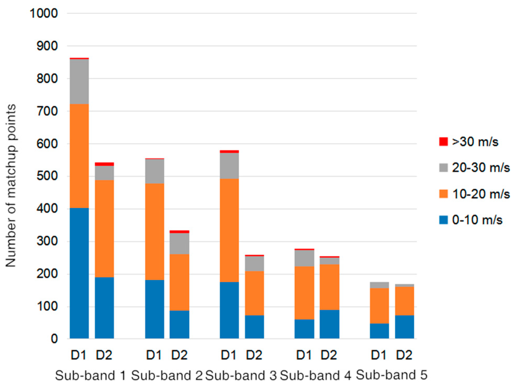
The S-1A images and SMAP references are divided into two datasets. Figure 3 shows the numbers of matching points in different wind ranges and different sub-bands. Both datasets cover wind speeds ranging from 5 to 35 m/s. There is a total of 4048 matching samples: 2476 in dataset 1 and 1572 in dataset 2. Note that, the width of sub-band 1 is larger than the widths of sub-bands 2–5 in range direction. For some images, there are no matching points in sub-bands 4 and 5. Therefore, the number of matching samples decreases from sub-bands 1 to 5.
3. Data Analyses
As mentioned above, the NRCS of VH-polarized signal is mainly dependent on wind speed and is barely dependent on wind direction and incidence angle, which makes VH-polarized images suitable for high wind retrieval. In this section, based on dataset 1, the relationships between VH NRCS, wind speed, wind direction, and incidence angle will be analyzed.
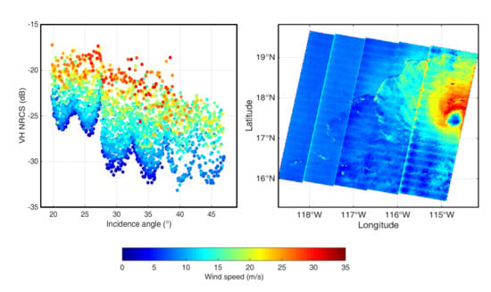
Figure 4 shows the relationships between VH NRCS and SMAP wind speed observations in different sub-bands. The wind ranges are 2–32 m/s, 2–35 m/s, 2–31 m/s, 7–32 m/s, and 7–24 m/s for sub-bands 1–5, respectively. The NRCS samples with different incidence angles cover the whole wind range in each sub-band.
As shown in Figure 4, the NRCS increases with wind speed in all sub-bands. For sub-bands 1–3, the NRCS increases linearly. For sub-bands 4 and 5, the slopes decrease in the entire wind ranges. Compared with sub-band 1, sub-bands 2–5 have lower NRCS levels under the same wind speed. The correlation coefficients (r) between NRCS and wind speed are 0.86, 0.91, 0.82, 0.76, and 0.78 for sub-bands 1–5, respectively. Based on the strong dependence of NRCS on wind speed, wind speed retrieval model will be presented in Section 4 for each sub-band.
The relationships between the VH-polarized NRCS and the incidence angle under different wind speeds are shown in Figure 5. For S-1A EW mode data, the incidence angles are about 19.75–27.55°, 27.55–32.55°, 32.55–37.95°, 37.95–42.85°, and 42.85–46.95° for sub-bands 1–5, respectively.
The features of NESZ mentioned above can also be found in Figure 5. For sub-band 1, the NRCS under the same wind speed has three peaks: one in the middle of the band and two at the boundaries. For sub-bands 2-5, the NRCS has a low level in the middle of the band and a high level at the inter-band boundaries. As is shown in Figure 5, the incidence angle has a strong influence on NRCS under low wind speed (<10 m/s). In addition, under the same wind speed level, the fluctuation of NRCS is up to 5 dB, which may influence the precision of the NRCS simulation and wind retrieval. According to the role of incidence angle in backscattering, the corrected functions of NRCS will be proposed in Section 4.
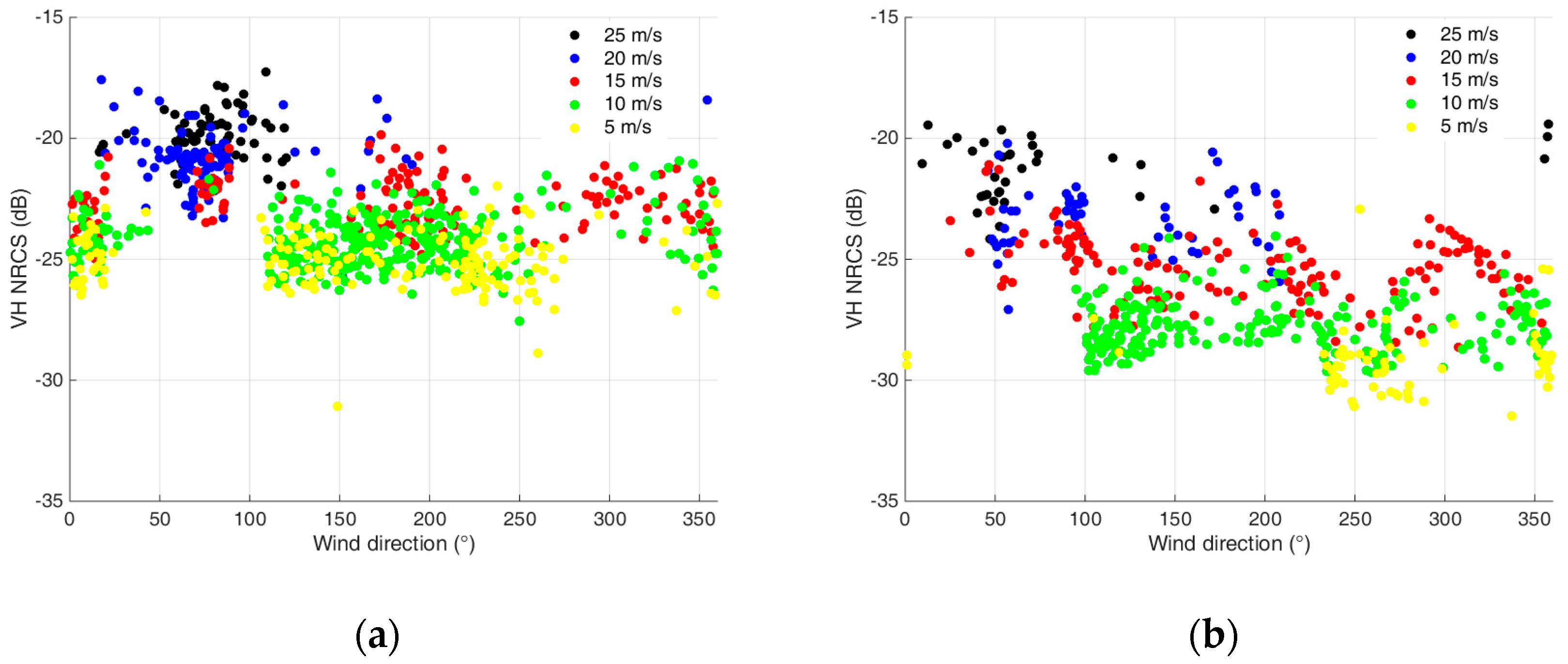
In GMF, the wind direction is the radar relative wind direction, which is the angle between the sea surface wind direction and radar azimuth look direction. Based on dataset 1, the scatterplots in Figure 6a–e show the distributions of NRCS for wind speeds at 5, 10, 15, 20, and 25 m/s with a range of ± 2.5 m/s in each sub-band. Then, the NRCS samples are averaged for wind speeds at 5, 10, 15, 20, and 25 m/s with a range of ± 2.5 m/s. The relationships between NRCS and wind direction under different wind speeds are shown in Figure 6f. The average NRCS values are calculated at different wind directions within a range of 15°.
As shown in Figure 6, the NRCS increases with wind speed and has an irregular fluctuation with the change of wind direction. The fluctuations under wind speeds 5 and 10 m/s are stronger than the fluctuations under wind speeds 15, 20, and 25 m/s. Since the incidence angle has a stronger influence on NRCS under low wind speeds, as shown in Figure 5. These phenomena indicate that the dependence of NRCS on incidence angle is stronger than on wind direction. Note that for the whole wind direction range (0–360°), the amount of matching data in dataset 1 is not enough to indicate the correlations between NRCS and wind direction under every incidence angles. Therefore, the dependence of NRCS on wind direction is assumed to be weak. In this paper, the wind direction factor is not considered in the construction of the model.
4. Wind Retrieval Model
4.1. Basic Model
According to the distribution of the data samples in Figure 4 and the strong correlation between VH-polarized NRCS and wind speed, linear function and power law function are used to fit the points for each sub-band. The fitting functions are linear functions for sub-bands 1–3 and power law functions for sub-bands 4 and 5. The fitting results are shown in Figure 7 (red curves). These basic empirical functions are proposed as:
where is the VH-polarized NRCS, represents the sea surface wind speed in 10-m height. The units of and are decibels and meters per second, respectively.
Based on the SMAP wind speeds in dataset 1, the NRCS values are simulated by the basic model to make a comparison with the observed NRCS. The comparisons between the observed and the simulated NRCS for each sub-band are shown in Figure 8 and Table 2. The correlation coefficients between the observed and the simulated NRCS are 0.83, 0.90, 0.82, 0.80, and 0.83 for sub-bands 1–5, respectively. The biases between the observed and the simulated NRCS are 0.06, −0.03, −0.06, −0.07, and 0.03 dB for sub-bands 1–5, respectively. The standard deviations (Std) between the observed and the simulated NRCS are 1.19, 1.19, 1.63, 1.62, and 1.38 dB for sub-bands 1–5, respectively. Through curve fitting, Equation (1) ensures that the bias of the simulation is minimized.
4.2. Corrected Model
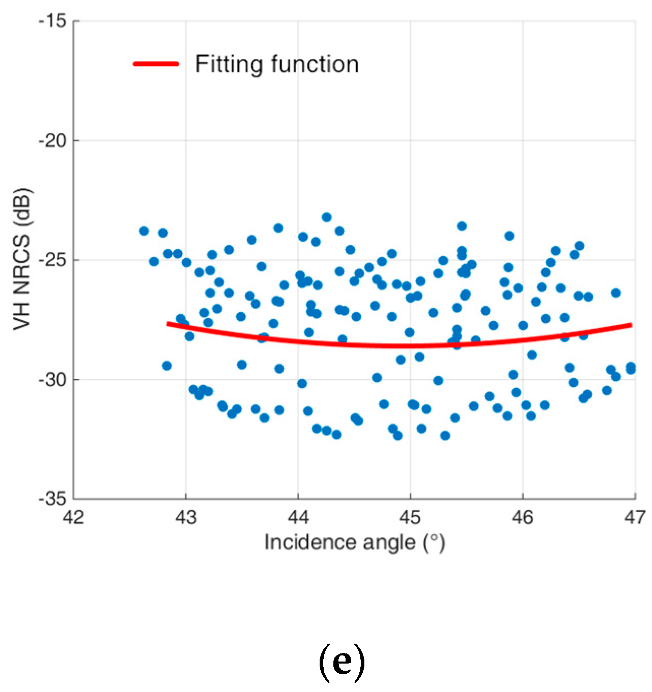
Based on the dependence of VH NRCS on radar incidence angle, the basic model is corrected in this section. Trigonometric function and quadratic function are used to fit the variations of NRCS with incidence angle for sub-band 1 and sub-bands 2–5, respectively. In this paper, the samples with wind speeds higher than 20 m/s are only 14.7% of all samples, thus, the curve fitting is only carried out for samples with wind speeds lower than 20 m/s. The fitting results are proposed as follows:
where is the VH-polarized NRCS, and represents the incidence angle. The units of and are decibels and degrees, respectively. The proposed fitting functions are shown in Figure 9.
In this paper, the proposed basic model is based on the average distribution of the matching data. Due to the fluctuation of NRCS with incidence angle, the retrieved wind speed from the basic model is too high at the peak of NRCS and too low at the trough of NRCS, leading to a high Std of wind retrieval. To minimize the Std, Equation (2) is used for making the fluctuation of NRCS as smooth as possible:
where N is the number of matching points for each sub-band in dataset 1, is the correction factor, and are the observed VH NRCS and incidence angles of the data samples. The units of and are decibels and degrees, respectively. During the Std minimization, the values are calculated at 4, 6, 8, 10, 12, 14, 16 and 18 m/s bounded by ±1 m/s interval. Based on linear fitting, the empirical function is:
Figure 10 shows the functions for each sub-band under different wind speeds. The correction factor decreases linearly with . The parameters , are reported in Table 3.
Based on Equations (1)–(4), Equation (5) is established to eliminate the overflow of NRCS in the process of Std minimization and decrease bias:
where is the SMAP wind speed in dataset 1. is the correction factor which is a function of wind speed. Linear functions are used to fit for each sub-band. The fitting parameters , are shown in Table 4.
Finally, a Std-minimized and bias-corrected wind retrieval model is proposed:
which is referred to as the corrected model. This model can be used for simulating NRCS of S-1A VH-polarized EW mode images or retrieving sea surface wind speeds up to 20 m/s from S-1A VH-polarized EW mode images. Figure 11 is an example of comparison between the basic model and the corrected model at 10 m/s wind speed.
5. Validation and Discussion
As mentioned previously, the basic wind retrieval model is a function of VH-polarized NRCS and sea surface wind speed. The corrected model is a function of VH-polarized NRCS, sea surface wind speed, and radar incidence angle. Based on dataset 2, the proposed basic model and corrected model are validated and discussed in this section.
5.1. Comparison of Basic Model and Corrected Model
Experiments are carried out to compare the retrieval performance of the basic model and the corrected model for wind speeds lower than 20 m/s. The results of each sub-band are illustrated in Figure 12 and Table 5. There are 489, 260, 209, 230, and 161 samples for sub-bands 1, 2, 3, 4, and 5, respectively.
The blue points in Figure 12 illustrate the comparison of wind speeds retrieved by basic model and wind speeds from SMAP. For sub-bands 1–5, the correlation coefficients are 0.68, 0.81, 0.87, 0.81, and 0.81, the Std are 4.17, 3.89, 3.75, 3.39, and 3.20 m/s, and the biases are −0.04, −0.49, −0.39, −0.47 and −0.35 m/s, respectively.
The comparison of retrieved wind speeds by the corrected model and the wind speeds from SMAP is illustrated by the red points in Figure 12. For sub-bands 1–5, the correlation coefficients are 0.79, 0.83, 0.89, 0.81, and 0.82, the Std are 3.50, 3.50, 3.18, 3.17, and 3.11 m/s, and the biases are 0.55, −0.81, −0.31, −0.10, and −0.46 m/s, respectively.
According to the retrieval results, the results of the basic model have smaller biases. However, the wind speeds retrieved by the corrected model have larger correlation coefficients and smaller Std. Due to the weaker dependence of NRCS on incidence angle in sub-bands 4 and 5, the decrease of Std is smaller in sub-bands 4 and 5 than in sub-bands 1–3.
A case study is carried out by retrieving wind speeds from the S-1A VH-polarized EW mode image of Tropical Storm Lester on 26 August 2016. The retrieved wind speed fields using the basic model and the corrected model are shown in Figure 13a,b. In Figure 13b, the wind speeds lower than 20 m/s are corrected with incidence angles. The collocated SMAP wind observation is shown in Figure 13c.
In Figure 13a, wind speeds are high at the boundaries of each sub-band and in the middle of sub-band 1. In Figure 13b, for wind speeds lower than 20 m/s, such phenomena are not as obvious as in Figure 13a, indicating the Std-minimization ability of the corrected model. In this case, the maximum wind speed retrieved by the basic model is 38.7 m/s. According to the National Hurricane Center (NHC)’s report, the maximum wind speed of Tropical Storm Lester was about 55–60 knots (28.3–30.9 m/s) at the SAR sensing time. The maximum retrieved wind speed is much higher than the NHC report. Therefore, the basic model is not recommended for retrieving wind speeds higher than 30 m/s. More samples are needed to explore the wind speed retrieval model under severe wind conditions in the future. In addition, the scalloping burstwise variation is maintained in the process of wind retrieval, showing some periodic streaks in sub-band 1 in Figure 13a,b.
5.2. Model Validation
In this section, the proposed model is compared with the MS1A model proposed by Mouche et al. [12]. The MS1A model is established with Sentinel-1A VH-polarized data and collocated wind speeds from SMAP:
MS1A model is a power law function. stands for the NRCS in linear scale. represents the 10-m height ocean surface wind speed corresponding to the transitions in the NRCS regime. and are dimensionless coefficients. The correlation coefficients, Std, and biases between the SMAP winds and the wind retrievals utilizing MS1A and the model proposed in this study are calculated for each sub-band. The comparison results are illustrated in Figure 14 and Table 6, showing that the retrieved wind speeds by the model proposed this study have higher correlation coefficients and lower Std and biases in most sub-bands. The large difference of retrieval results of the two models is mainly caused by the quality of the SMAP data and the SAR data used in the two studies. On one hand, Mouche et al. used SMAP brightness temperature data to compute the wind speeds. In this paper, SMAP Level-2 data are downloaded and then used directly. On the other hand, the NRCS values they used seem to be higher than ours. In [12], there are many NRCS observations below the NESZ values, leading to higher retrieval results by MS1A as measured by the SMAP Level-2 dataset.
5.3. Error Analyses
Under tropical cyclone conditions, low spatial resolution will lead to a smoothed wind field, potentially missing small regions with high wind speeds. Due to the resolution difference between the S-1A data and the SMAP data, the pixel number of S-1A image used for averaging might influence the retrieval results. In order to evaluate the performance of the proposed model for datasets with different pixel numbers, wind speeds are retrieved from dataset 2 with an averaging of 8 × 8, 16 × 16, 32 × 32, 64 × 64, 128 × 128, 256 × 256, and 512 × 512 pixels in one cell, respectively. Correlation coefficient, Std, and bias between the retrieved wind speeds and the SMAP winds are illustrated in Table 7, showing the stability of the proposed model. In addition, the number of matching data might influence the experiment results, especially under strong-to-severe wind conditions in this study. The proposed model can be improved when more observations with higher spatial resolution (for example SFMR or H*Wind) become available in the future.
In this paper, the methodology and the accuracy of data could influence the parameters of the proposed model and the validation results. On one hand, the methodology of noise removal could lead to an error of NRCS. The S-1A VH-polarized EW mode data have noise variation in the azimuth direction, called azimuth scalloping [24]. The areas near the burst edges are brighter than those in the burst center because of their higher noise power of azimuth scalloping. The azimuth scalloping attenuates from sub-bands 1 to 5. In sub-band 1, the azimuth scalloping can lead to an error of NRCS up to 1.5 dB. In this study, a large number of S-1A images are collected to minimize the azimuth scalloping error.
On the other hand, tropical cyclones are always accompanied with rainfall which can strongly dampen the NRCS, leading to significant underestimates in wind speeds [18,27]. In this study, there is no matching data for precipitation. As mentioned in Section 3, the proposed model has a low slope under strong-to-severe wind speeds for sub-bands 4 and 5. According to the proposed model, a NRCS error of 1 dB might cause a wind retrieval error up to 5 m/s. In addition, the SMAP wind speeds and WindSat observations have a global RMS of 1.5 m/s, which might influence the precision of the proposed model.
Finally, the collocation time difference is very important for modeling and validation. Requiring a smaller time difference may lead to a reduced, and insufficient quantity of data samples. In this paper, if the time difference is restricted to 30 min, nearly half of the samples will be lost. It will be difficult to propose and validate the retrieval model, especially for high wind speeds. However, if the time difference is increased to more than one hour or even two hours, the motion of tropical cyclones and the variation of wind fields will influence the accuracy of wind retrieval. If more hurricane SAR images could be acquired in the future, the time difference could be reduced. In addition, experiments could also be made to test to what extent the collocation time difference influences modeling.
6. Conclusions
In this paper, a new model is developed for retrieving sea surface wind speed from S-1A EW mode VH-polarized images. 19 noise-free S-1A images and matching data from SMAP radiometer under tropical cyclone conditions are collected and analyzed. According to 12 S-1A images and matching data, the VH NRCS has a strong correlation with wind the speeds in each sub-band of the S-1A images. With the change of incidence angle, the VH NRCS has a high level at the boundaries of each sub-band and in the middle of sub-band 1.
Based on the relationship between VH NRCS and wind speed, a basic model is proposed to construct a wind retrieval model. In addition, a corrected model is proposed to improve the accuracy of the basic model, according to the relationship between NRCS and incidence angle.
In order to validate the validity of the wind retrieval model, the wind speeds retrieved by the corrected model are compared with the wind speeds retrieved by the basic model and the MS1A model in 7 S-1A images. A case study is also carried out by retrieving the wind speed field from the S-1A image of Tropical Storm Lester. Validating against the winds from SMAP, the wind speeds retrieved by the corrected model are more accurate than the basic model for wind speeds lower than 20 m/s, especially in the middle of the sub-band and at the inter-band boundaries.
For sub-bands 1–5, the correlation coefficients, Std, and biases between the retrieved winds and the SMAP winds are 0.68–0.89, 3.11–4.17 m/s, and −0.81–0.55 m/s, respectively. The retrieval results are fairly accurate, indicating that the proposed wind speed retrieval model is reliable. Finally, error sources of the proposed model and our experiments are analyzed with respect to the proposed methodology and the matching data.
Author Contributions
Initiation of the idea: Y.G. and J.S.; data processing and model proposing: Y.G.; writing and editing: all authors contributed; supervision: L.X.; funding acquisition: J.S. and C.G.
Funding
This research was funded by National Key Research and Development Program of China under grant number 2016YFC1401405 and the National Science Foundation of China under grant number 41376010.
Acknowledgments
The authors would like to thank the European Space Agency for making Sentinel-1A data publicly available. We thank the National Aeronautics and Space Administration for the SMAP data, and the National Hurricane Center for its hurricane report.
Conflicts of Interest
The authors declare no conflict of interest.
References
- Hwang, P.A.; Fois, F. Surface roughness and breaking wave properties retrieved from polarimetric microwave radar backscattering. J. Geophys. Res. Oceans 2015, 120, 3640–3657. [Google Scholar] [CrossRef] [Green Version]
- Monaldo, F.M.; Jackson, C.; Li, X. On the use of Sentinel-1 cross-polarization imagery for wind speed retrieval. In Proceedings of the 2017 IEEE International Geoscience and Remote Sensing Symposium, Fort Worth, TX, USA, 23–28 July 2017; pp. 392–395. [Google Scholar]
- Gerling, T. Structure of the surface wind field from the Seasat SAR. J. Geophys. Res. Oceans 1986, 91, 2308–2320. [Google Scholar] [CrossRef]
- Alpers, W.; Brümmer, B. Atmospheric boundary layer rolls observed by the synthetic aperture radar aboard the ERS-1 satellite. J. Geophys. Res. Oceans 1994, 99, 12613–12621. [Google Scholar] [CrossRef]
- Du, Y.; Vachon, P.W.; Wolfe, J. Wind direction estimation from SAR images of the ocean using wavelet analysis. Can. J. Remote Sens. 2002, 28, 498–509. [Google Scholar] [CrossRef]
- Gao, Y.; Guan, C.; Sun, J.; Xie, L. A New Hurricane Wind Direction Retrieval Method for SAR Images without Hurricane Eye. J. Atmos. Ocean. Technol. 2018, 35, 2229–2239. [Google Scholar] [CrossRef]
- Shen, H.; He, Y.; Perrie, W. Speed ambiguity in hurricane wind retrieval from SAR imagery. Int. J. Remote Sens. 2009, 30, 2827–2836. [Google Scholar] [CrossRef]
- Valenzuela, G. Depolarization of EM waves by slightly rough surfaces. IEEE Trans. Antennas Propag. 1967, 15, 552–557. [Google Scholar] [CrossRef]
- Voronovich, A.G.; Zavorotny, V.U. Depolarization of microwave backscattering from a rough sea surface: Modeling with small-slope approximation. In Proceedings of the 2011 IEEE International Geoscience and Remote Sensing Symposium (IGARSS), Vancouver, BC, Canada, 24–29 July 2011; pp. 2033–2036. [Google Scholar]
- Voronovich, A.G.; Zavorotny, V.U. Full-polarization modeling of monostatic and bistatic radar scattering from a rough sea surface. IEEE Trans. Antennas Propag. 2014, 62, 1362–1371. [Google Scholar] [CrossRef]
- Hwang, P.A.; Stoffelen, A.; Zadelhoff, G.J.; Perrie, W.; Zhang, B.; Li, H.; Shen, H. Cross-polarization geophysical model function for C-band radar backscattering from the ocean surface and wind speed retrieval. J. Geophys. Res. Oceans 2015, 120, 893–909. [Google Scholar] [CrossRef] [Green Version]
- Mouche, A.A.; Chapron, B.; Zhang, B.; Husson, R. Combined co-and cross-polarized SAR measurements under extreme wind conditions. IEEE Trans. Geosci. Remote Sens. 2017, 55, 6746–6755. [Google Scholar] [CrossRef]
- Hwang, P.A.; Zhang, B.; Perrie, W. Depolarized radar return for breaking wave measurement and hurricane wind retrieval. Geophys. Res. Lett. 2010, 37, L01604. [Google Scholar] [CrossRef]
- Zhang, B.; Perrie, W.; He, Y. Wind speed retrieval from RADARSAT-2 quad-polarization images using a new polarization ratio model. J. Geophys. Res. Oceans 2011, 116, C08008. [Google Scholar] [CrossRef]
- Vachon, P.W.; Wolfe, J. C-band cross-polarization wind speed retrieval. IEEE Trans. Geosci. Electron. Lett. 2011, 8, 456–459. [Google Scholar] [CrossRef]
- Zhang, B.; Perrie, W.; Zhang, J.A.; Uhlhorn, E.W.; He, Y. High-resolution hurricane vector winds from C-band dual-polarization SAR observations. J. Atmos. Ocean. Technol. 2014, 31, 272–286. [Google Scholar] [CrossRef]
- Horstmann, J.; Falchetti, S.; Wackerman, C.; Maresca, S.; Caruso, M.J.; Graber, H.C. Tropical cyclone winds retrieved from C-band cross-polarized synthetic aperture radar. IEEE Trans. Geosci. Remote Sens. 2015, 53, 2887–2898. [Google Scholar] [CrossRef]
- Zhang, B.; Perrie, W. Cross-Polarized Synthetic Aperture Radar: A New Potential Measurement Technique for Hurricanes. Bull. Am. Meteorol. Soc. 2012, 93, 531–541. [Google Scholar] [CrossRef] [Green Version]
- Zadelhoff, G.J.V.; Stoffelen, A.; Vachon, P.W.; Wolfe, J.; Horstmann, J.; Rivas, M.B. Scatterometer hurricane wind speed retrievals using cross polarization. Atmos. Meas. Tech. Discuss. 2013, 6, 7945–7984. [Google Scholar] [CrossRef]
- Zhang, G.; Li, X.; Perrie, W.; Hwang, P.A.; Zhang, B.; Yang, X. A hurricane wind speed retrieval model for C-band RADARSAT-2 cross-polarization ScanSAR images. IEEE Trans. Geosci. Remote Sens 2017, 55, 4766–4774. [Google Scholar] [CrossRef]
- Huang, L.; Liu, B.; Li, X.; Zhang, Z.; Yu, W. Technical evaluation of Sentinel-1 IW mode cross-pol radar backscattering from the ocean surface in moderate wind condition. Remote Sens. 2017, 9, 854. [Google Scholar] [CrossRef]
- Zhou, X.; Yang, X.; Li, Z.; Yu, Y.; Bi, H.; Ma, S.; Li, X. Estimation of tropical cyclone parameters and wind fields from SAR images. Sci. China Earth Sci. 2013, 56, 1977–1987. [Google Scholar] [CrossRef]
- Shao, W.; Li, X.; Hwang, P.; Zhang, B.; Yang, X. Bridging the gap between cyclone wind and wave by C-band SAR measurements. J. Geophys. Res. Oceans 2017, 122, 6714–6724. [Google Scholar] [CrossRef]
- Park, J.-W.; Korosov, A.A.; Babiker, M.; Sandven, S.; Won, J.-S. Efficient Thermal Noise Removal for Sentinel-1 TOPSAR Cross-Polarization Channel. IEEE Trans. Geosci. Remote Sens. 2018, 56, 1555–1565. [Google Scholar] [CrossRef]
- Meissner, T.; Ricciardulli, L.; Wentz, F.J. Capability of the SMAP Mission to Measure Ocean Surface Winds in Storms. Bull. Am. Meteorol. Soc. 2017, 98. [Google Scholar] [CrossRef]
- Fore, A.; Yueh, S.; Tang, W.; Stiles, B.; Hayashi, A. Validation of SMAP radiometer extreme wind speed data product with rapid scatterometer and stepped frequency microwave radiometer. In Proceedings of the 2017 IEEE International Geoscience and Remote Sensing Symposium, Fort Worth, TX, USA, 23–28 July 2017; pp. 398–401. [Google Scholar]
- Powell, M.D. Boundary layer structure and dynamics in outer hurricane rainbands. Part I: Mesoscale rainfall and kinematic structure. Mon. Weather Rev. 1990, 118, 891–917. [Google Scholar] [CrossRef]
Figure 1.
The distributions of NESZ and incidence angle in sub-bands 1 to 5.

Figure 2.
The variation of NRCS Std with different calculation resolutions.

Figure 3.
The numbers of matching points in different wind ranges and different sub-bands. D1 is an abbreviation of dataset 1 and D2 is an abbreviation of dataset 2.
Figure 3.
The numbers of matching points in different wind ranges and different sub-bands. D1 is an abbreviation of dataset 1 and D2 is an abbreviation of dataset 2.

Figure 4.
Relationships between VH NRCS and SMAP wind speed for (a) sub-band 1, (b) sub-band 2, (c) sub-band 3, (d) sub-band 4, and (e) sub-band 5. N is the number of matching points and r stands for the correlation coefficient.
Figure 4.
Relationships between VH NRCS and SMAP wind speed for (a) sub-band 1, (b) sub-band 2, (c) sub-band 3, (d) sub-band 4, and (e) sub-band 5. N is the number of matching points and r stands for the correlation coefficient.

Figure 5.
The relationship between VH NRCS and incidence angle under different wind speeds.

Figure 6.
The relationships between VH NRCS and wind direction under different wind speeds for (a) sub-band 1, (b) sub-band 2, (c) sub-band 3, (d) sub-band 4, and (e) sub-band 5. (f) The variation of average VH NRCS with wind direction under different wind speeds.
Figure 6.
The relationships between VH NRCS and wind direction under different wind speeds for (a) sub-band 1, (b) sub-band 2, (c) sub-band 3, (d) sub-band 4, and (e) sub-band 5. (f) The variation of average VH NRCS with wind direction under different wind speeds.


Figure 7.
Fitting functions (red curves) between VH NRCS and SMAP wind speeds for (a) sub-band 1, (b) sub-band 2, (c) sub-band 3, (d) sub-band 4, and (e) sub-band 5.
Figure 7.
Fitting functions (red curves) between VH NRCS and SMAP wind speeds for (a) sub-band 1, (b) sub-band 2, (c) sub-band 3, (d) sub-band 4, and (e) sub-band 5.

Figure 8.
Comparisons between simulated VH NRCS and observed VH NRCS for (a) sub-band 1, (b) sub-band 2, (c) sub-band 3, (d) sub-band 4, and (e) sub-band 5. N, r, Std, Bias represents the number of matching points, correlation coefficient, standard deviation, and bias between observed NRCS and simulated NRCS with the proposed basic model.

Figure 9.
Fitting functions (red curves) between VH NRCS and incidence angle for (a) sub-band 1, (b) sub-band 2, (c) sub-band 3, (d) sub-band 4, and (e) sub-band 5.
Figure 9.
Fitting functions (red curves) between VH NRCS and incidence angle for (a) sub-band 1, (b) sub-band 2, (c) sub-band 3, (d) sub-band 4, and (e) sub-band 5.


Figure 10.
The empirical functions for each sub-band under different wind speeds.

Figure 11.
The comparison between basic model and corrected model at 10 m/s wind speed.

Figure 12.
SAR-retrieved wind speeds with basic model and corrected model vs SMAP wind speeds in (a) sub-band 1, (b) sub-band 2, (c) sub-band 3, (d) sub-band 4, and (e) sub-band 5.
Figure 12.
SAR-retrieved wind speeds with basic model and corrected model vs SMAP wind speeds in (a) sub-band 1, (b) sub-band 2, (c) sub-band 3, (d) sub-band 4, and (e) sub-band 5.


Figure 13.
Retrieved sea surface wind speed of Tropical Storm Lester using (a) basic model, (b) basic model and corrected model, and (c) SMAP wind observation.
Figure 13.
Retrieved sea surface wind speed of Tropical Storm Lester using (a) basic model, (b) basic model and corrected model, and (c) SMAP wind observation.


Figure 14.
SAR-retrieved wind speeds by our model (red points) and MS1A model (blue points) vs SMAP wind speeds in (a) sub-band 1, (b) sub-band 2, (c) sub-band 3, (d) sub-band 4, and (e) sub-band 5.
Figure 14.
SAR-retrieved wind speeds by our model (red points) and MS1A model (blue points) vs SMAP wind speeds in (a) sub-band 1, (b) sub-band 2, (c) sub-band 3, (d) sub-band 4, and (e) sub-band 5.


Table 1.
S-1A data information.
| Tropical Cyclone Name | Sensing Time (UTC) | Number of Matching Points | Dataset |
|---|---|---|---|
| Lester | 2016-08-26 13:39 | 241 | 1 |
| Lester | 2016-08-30 14:45 | 202 | 1 |
| Lester | 2016-08-31 03:15 | 184 | 1 |
| Gaston | 2016-08-27 09:22 | 257 | 2 |
| Gaston | 2016-08-29 21:41 | 112 | 2 |
| Gaston | 2016-08-29 21:42 | 125 | 2 |
| Gaston | 2016-09-01 20:29 | 279 | 2 |
| Lionrock | 2016-08-27 20:52 | 225 | 1 |
| Lionrock | 2016-08-29 20:34 | 264 | 2 |
| Lionrock | 2016-08-29 20:35 | 263 | 1 |
| Namtheum | 2016-09-04 09:20 | 253 | 2 |
| Hermine | 2016-09-04 22:31 | 279 | 1 |
| Hermine | 2016-09-04 22:32 | 282 | 2 |
| Karl | 2016-09-23 22:22 | 176 | 1 |
| Karl | 2016-09-23 22:23 | 171 | 1 |
| Karl | 2016-09-24 10:25 | 154 | 1 |
| Karl | 2016-09-24 10:26 | 166 | 1 |
| Karl | 2016-09-24 10:27 | 183 | 1 |
| Megi | 2016-09-26 09:34 | 232 | 1 |
Table 2.
Correlation coefficient, Std and bias between the observed NRCS and the simulated NRCS with basic model.
Table 2.
Correlation coefficient, Std and bias between the observed NRCS and the simulated NRCS with basic model.
| Sub-Band | r | Std (dB) | Bias (dB) |
|---|---|---|---|
| 1 | 0.83 | 1.19 | 0.06 |
| 2 | 0.90 | 1.19 | −0.03 |
| 3 | 0.82 | 1.63 | −0.06 |
| 4 | 0.80 | 1.62 | −0.07 |
| 5 | 0.83 | 1.38 | 0.03 |
Table 3.
Parameters for Equation (4).
| Sub-Band | ||
|---|---|---|
| 1 | −0.06 | 1.71 |
| 2 | −0.10 | 2.29 |
| 3 | −0.09 | 2.04 |
| 4 | −0.14 | 2.66 |
| 5 | −0.11 | 2.47 |
Table 4.
Parameters for Equation (6).
| Sub-Band | ||
|---|---|---|
| 1 | −1.55 | 41.35 |
| 2 | −2.63 | 61.28 |
| 3 | −2.44 | 55.43 |
| 4 | −3.70 | 72.42 |
| 5 | −3.02 | 69.70 |
Table 5.
Correlation coefficient, Std, and bias between wind speed from SMAP and retrieved wind speed with basic model and corrected model.
Table 5.
Correlation coefficient, Std, and bias between wind speed from SMAP and retrieved wind speed with basic model and corrected model.
| Sub-Band | r | Std (m/s) | Bias (m/s) | |||
|---|---|---|---|---|---|---|
| Basic Model | Corrected Model | Basic Model | Corrected Model | Basic Model | Corrected Model | |
| 1 | 0.68 | 0.79 | 4.17 | 3.50 | −0.04 | 0.55 |
| 2 | 0.81 | 0.83 | 3.89 | 3.50 | −0.49 | −0.81 |
| 3 | 0.87 | 0.89 | 3.75 | 3.18 | −0.39 | −0.31 |
| 4 | 0.81 | 0.81 | 3.39 | 3.17 | −0.47 | −0.10 |
| 5 | 0.81 | 0.82 | 3.20 | 3.11 | −0.35 | −0.46 |
Table 6.
Correlation coefficient, Std and bias between wind speeds from SMAP and retrieved wind speeds by our model and MS1A model.
Table 6.
Correlation coefficient, Std and bias between wind speeds from SMAP and retrieved wind speeds by our model and MS1A model.
| Sub-Band | r | Std (m/s) | Bias (m/s) | |||
|---|---|---|---|---|---|---|
| Our Model | MS1A Model | Our Model | MS1A Model | Our Model | MS1A Model | |
| 1 | 0.87 | 0.75 | 3.66 | 4.84 | 0.45 | −7.38 |
| 2 | 0.87 | 0.70 | 3.79 | 5.35 | −0.47 | −3.85 |
| 3 | 0.92 | 0.87 | 3.10 | 3.41 | −0.36 | −3.47 |
| 4 | 0.88 | 0.88 | 3.56 | 2.67 | −0.56 | −3.52 |
| 5 | 0.85 | 0.83 | 3.43 | 2.45 | −0.69 | −3.73 |
Table 7.
Performance of the model for dataset with different pixel number.
| Pixel Number | r | Std (m/s) | Bias (m/s) |
|---|---|---|---|
| 8 × 8 | 0.86 | 3.42 | −0.31 |
| 16 × 16 | 0.88 | 3.51 | −0.3 |
| 32 × 32 | 0.90 | 3.31 | −0.38 |
| 64 × 64 | 0.89 | 3.20 | −0.27 |
| 128 × 128 | 0.87 | 3.40 | −0.30 |
| 256 × 256 | 0.88 | 3.59 | 0.12 |
| 512 × 512 | 0.92 | 3.63 | 0.09 |
© 2019 by the authors. Licensee MDPI, Basel, Switzerland. This article is an open access article distributed under the terms and conditions of the Creative Commons Attribution (CC BY) license (http://creativecommons.org/licenses/by/4.0/).
Share and Cite
MDPI and ACS Style
Gao, Y.; Guan, C.; Sun, J.; Xie, L. A Wind Speed Retrieval Model for Sentinel-1A EW Mode Cross-Polarization Images. Remote Sens. 2019, 11, 153. https://doi.org/10.3390/rs11020153
AMA Style
Gao Y, Guan C, Sun J, Xie L. A Wind Speed Retrieval Model for Sentinel-1A EW Mode Cross-Polarization Images. Remote Sensing. 2019; 11(2):153. https://doi.org/10.3390/rs11020153
Chicago/Turabian StyleGao, Yuan, Changlong Guan, Jian Sun, and Lian Xie. 2019. "A Wind Speed Retrieval Model for Sentinel-1A EW Mode Cross-Polarization Images" Remote Sensing 11, no. 2: 153. https://doi.org/10.3390/rs11020153
Note that from the first issue of 2016, this journal uses article numbers instead of page numbers. See further details here.