Satellite Retrieval of Downwelling Shortwave Surface Flux and Diffuse Fraction under All Sky Conditions in the Framework of the LSA SAF Program (Part 1: Methodology)

Abstract

Several studies have shown that changes in incoming solar radiation and variations of the diffuse fraction can significantly modify the vegetation carbon uptake. Hence, monitoring the incoming solar radiation at large scale and with high temporal frequency is crucial for this reason along with many others. The European Organization for the Exploitation of Meteorological Satellites (EUMETSAT) Satellite Application Facility for Land Surface Analysis (LSA SAF) has operationally disseminated in near real time estimates of the downwelling shortwave radiation at the surface since 2005. This product is derived from observations provided by the SEVIRI instrument onboard the Meteosat Second Generation series of geostationary satellites, which covers Europe, Africa, the Middle East, and part of South America. However, near real time generation of the diffuse fraction at the surface level has only recently been initiated. The main difficulty towards achieving this goal was the general lack of accurate information on the aerosol particles in the atmosphere. This limitation is less important nowadays thanks to the improvements in atmospheric numerical models. This study presents an upgrade of the LSA SAF operational retrieval method, which provides the simultaneous estimation of the incoming solar radiation and its diffuse fraction from the satellite every 15 min. The upgrade includes a comprehensive representation of the influence of aerosols based on physical approximations of the radiative transfer within an atmosphere-surface associated medium. This article explains the retrieval method, discusses its limitations and differences with the previous method, and details the characteristics of the output products. A companion article will focus on the evaluation of the products against independent measurements of solar radiation. Finally, the access to the source code is provided through an open access platform in order to share the expertise on the satellite retrieval of this variable with the community.

1. Introduction

The downwelling surface shortwave flux (DSSF) refers to the radiative energy in the wavelength interval [0.3 μm, 4.0 μm] that reaches the Earth’s surface per time unit and per surface area unit. DSSF essentially depends on the solar zenith angle, cloud coverage, aerosol load and type, and, to a lesser extent, gas absorption (water vapor, ozone content) and surface albedo. A study conducted by reference [1] showed the importance of clouds for the DSSF and the Earth’s energy budget at the surface level. Other studies have stressed the role of the energy budget at the surface level on weather forecasting and climate modeling (e.g., references [2,3,4,5]).

Solar radiation at the surface level is the first driver of the energy budget. However, the knowledge of the partitioning between its diffuse and direct components is also crucial. In this context, diffuse fraction is defined as the ratio between the diffuse component of DSSF and the total DSSF reaching the surface. Diffuse fraction is an important variable to understand the climate processes at the Earth-atmosphere interface, and especially to estimate plant photosynthesis and carbon cycle. For example, diffuse conditions let more sunlight strike the inner part of the canopy [6], which may induce an increase of the carbon uptake by the vegetation [7], although very high diffuse fractions are associated with a reduction in global radiation, which may negatively impact photosynthetic activity [7,8]. The ratio between diffuse and direct DSSF is also a fundamental attribute for the solar energy sector to predict the energy supply [9]. Diffuse fraction depends to a large extent on the presence of aerosols and clouds in the atmosphere. Because these two elements rapidly change with time and space, the accurate retrieval of diffuse fraction has proven to be very challenging so far.

Despite its interest, retrieval of diffuse fraction at large scales using satellites observations has been poorly considered until now. Nevertheless, reference [10] showed that the use of satellite observations from geostationary platforms offers an interesting opportunity to monitor the evolution of the incoming solar radiation at a high temporal frequency. Even if the variation of aerosol properties were not considered, reference [10] showed that satellite data can offer robust and accurate estimates in case of relatively pure atmosphere. Prior to their work, the scientific community developed several algorithms for the estimation of the downward and net surface solar irradiance from satellite observations (e.g., references [11,12,13,14,15,16,17,18,19,20,21,22,23,24,25]). However, to the best of our knowledge, there is no equivalent estimate of the diffuse fraction of the incoming solar radiation at the surface level made available freely to the community in near real time. Indeed, near-real time estimates of the instantaneous DSSF and its diffuse fractions are available from the Helioclim-3 data base [26,27,28], every 15 min over the MSG disk through paying for access.

The EUMETSAT (European Organization for the Exploitation of Meteorological Satellites) Satellite Application Facility (SAF) on Land Surface Analysis (LSA; [29]) is a part of the SAF Network, a set of specialized development and processing centers, serving as a EUMETSAT distributed Applications Ground Segment. The SAF network complements the product-oriented activities at the EUMETSAT Central Facility in Darmstadt. The eight EUMETSAT SAFs provide users with operational data and software products, each one for a dedicated user community and application area. For example, the Climate Monitoring (CM) SAF generates datasets for specific climate applications areas. User needs in this case require highly accurate and stable products, i.e., products based on input data (typically, reanalyses of modeled atmospheric water vapor and pressure) with a temporal consistency over several decades. On the other hand, the main purpose of the LSA SAF is to address the needs of the scientific communities that require land surface variables in a near-real time basis (i.e., with low latency times). Overall, LSA SAF products find applications in meteorology (numerical weather prediction), the solar energy sector, hydrology and environmental monitoring, among with by other users. Observations provided by the Spinning Enhanced Visible and Infrared Imager (SEVIRI) radiometer embarked on Meteosat Second Generation (MSG) geostationary satellites have been available since 2004. Considering the overall period it has been operational, SEVIRI encompasses unique spectral characteristics and accuracy: a 3 km spatial resolution at nadir (1 km for the high-resolution visible panchromatic channel), an imaging-repeat cycle of 15 min, and 12 spectral channels [30]. The catalogue of the LSA SAF products is available on the LSA SAF website (http://lsa-saf.eumetsat.int). These products have all been intensively validated against ground measurements, model outputs, or similar parameters retrieved from other sensors.

The list of LSA SAF products includes two DSSF products derived from MSG/SEVIRI data and developed based on the research conducted by reference [10]: the MDSSF product (referenced LSA-201) corresponding to instantaneous values of DSSF, and the DIDSSF product (LSA-203) corresponding to daily accumulated values of DSSF. Their distribution is performed in near real time with a timeliness of three hours, counted after the last satellite observation. The production is done every 30 min for the instantaneous MDSSF product, and daily for the DIDSSF product. Both products consider clear and cloudy skies, and provide total shortwave fluxes but without distinction of the diffuse fraction. Although these products have proven to be of high quality [31,32,33], they still show some limitations under clear-sky conditions, as they rely on the hypothesis of temporally and spatially constant aerosol properties [34]. The importance of aerosols on the DSSF estimation was underlined in numerous studies, especially in regions with high aerosol concentrations [35,36,37,38]. The main difficulty of using aerosols to derive DSSF was the general lack of accurate and dynamic information on the aerosol particles in the atmosphere. This limitation is nowadays less important thanks to the improvements in atmospheric numerical models combined with the use of an increase amount of satellite measurements [39,40,41]. Satellite products on aerosol properties (e.g., reference [42]) could represent alternatives. However, it was proved that their accuracy was still not enough to calculate accurately the radiative forcing due to aerosol at the surface [43], which is intimately related to DSSF.

This study describes the generation of a new LSA SAF product, referenced as LSA-207 and called the MSG-derived Downwelling Surface Shortwave Flux—Total and Diffuse (MDSSFTD). The two main advantages of this upgrade of the MDSSF operational product are (i) the improvement of the DSSF estimation (especially thanks to the consideration of the influence of aerosols on the atmospheric transmittance in case of clear-sky and cloudy-sky conditions), and (ii) the retrieval of the diffuse fraction at the surface level for all sky situations.

This article is organized as follows. Section 2 gives an overview of the methodology as well as the workflow for the estimation of the DSSF flux and its related fraction of diffuse radiation. Section 3 describes the input data that are needed for the calculation of these variables. Section 4 provides detailed descriptions of the algorithm under clear-sky and cloudy-sky conditions. Section 5 describes the characteristics of the product outputs and lists the known limitations before concluding in Section 6.

2. Method

2.1. Definition of Retrieved Quantities

2.1.1. Downwelling Surface Shortwave Radiation

The downwelling surface shortwave radiation flux, $E^{\downarrow }$, is defined as the integral of the spectral irradiance $E\left(\lambda \right)$ over the wavelength interval [$\lambda$₁ = 0.3 µm, $\lambda$₂ = 4 µm]

$$E^{\downarrow }={\displaystyle {\int }_{{\lambda }_1}^{{\lambda }_2}}E\left(\lambda \right)d\lambda$$

(1)

DSSF is expressed in Watts per square meter (W/m²). The spectral irradiance at wavelength λ is the hemispherical angular integral of the downwelling spectral radiance $L\left(\lambda ,{\theta }_s,{\phi }_s\right)$ over the solar azimuth and zenith angles, noted respectively as ${\phi }_s$ and ${\theta }_s$, weighted by the cosine of the solar zenith angle

$$E\left(\lambda \right)={\displaystyle {\int }_{{\phi }_s=0}^{2\pi }}{\displaystyle {\int }_{{\theta }_s=0}^{\pi /2}}L\left(\lambda ,{\theta }_s,{\phi }_s\right)\cos \left({\theta }_s\right)\sin \left({\theta }_s\right)d{\theta }_{s}d{\phi }_s.$$

(2)

It includes contributions owing to the direct solar radiation ($E_{dir}$) attenuated by the atmosphere as well as diffuse radiation coming from other directions ($E_{dif}$):

$$E\left(\lambda \right)=E_{dir}\left(\lambda \right)+E_{dif}\left(\lambda \right)$$

(3)

The DSSF can be expressed as

$$E^{\downarrow }=E_{0}v\left(t\right)\cos {\theta }_{s}T,$$

(4)

where $E_0$ is the solar constant, ${\theta }_s$ is the solar zenith angle, v(t) is the Sun-Earth distance factor, and $T$ is the total effective transmittance of the entire atmosphere (including the cloud attenuation in the case of cloudy skies). The latter quantity can be decomposed into multiple attenuation processes of individual atmospheric components such as absorption by gases ($T_{gases}$), Rayleigh scattering ($T_{Ray}$), aerosols extinction ($T_{aer}$), and cloud extinction ($T_C$). The total transmittance is further detailed in Section 4.1.

The total DSSF, $E^{\downarrow }$, includes the contributions owing to the direct solar radiation attenuated by the atmosphere, as well as diffuse radiation. It can be approximated as

$$E^{\downarrow }=E_{0}v\left(t\right)\cos \left({\theta }_s\right)\left(T_{dir}+T_{dif}\right)=E_{dir}+E_{dif},$$

(5)

where $T_{dir}$ and $T_{dif}$ are the effective transmittances of the atmosphere system (cloud-gas-aerosol) for the direct and diffuse radiation, respectively, and $E_{dir}$ and $E_{dif}$ are the corresponding direct and diffuse radiation that compose the total DSSF.

2.1.2. Diffuse Fraction

The diffuse fraction, $f_d$, is the ratio between the diffuse incoming radiation and the total incoming radiation and is calculated as follows

$$f_d=\frac{{\displaystyle {\int }_{{\lambda }_1}^{{\lambda }_2}}{E}_{dif}\left(\lambda \right)d\lambda }{{\displaystyle {\int }_{{\lambda }_1}^{{\lambda }_2}}E\left(\lambda \right)d\lambda }.$$

(6)

This ratio is calculated at the surface level and for the visible broadband domain ([$\lambda$₁ = 0.3 µm, $\lambda$₂ = 4 µm]).

2.1.3. Equivalent Aerosol Optical Depth at 550 nm

The equivalent Aerosol Optical Depth (AOD) at 550 nm is related to the extinction of the solar beam by aerosol particles in the wavelength 550 nm. It takes into account the extinctions from different aerosols components that may co-exist in the same aerosol mixture (sulfates, sea salt, black carbon, etc.). Therefore, the equivalent AOD is linked to the extinction of the total column of atmosphere in presence of an unclassified aerosol mixture at 550 nm.

2.1.4. Opacity Index

The opacity of the atmosphere is by construction the opposite of the clearness. The Opacity Index ($OI$) is defined as

$$OI=1-K_t$$

(7)

where $Kt$ is the clearness index, in turn defined as the fraction of the solar radiation that is transmitted through the atmosphere to finally strike the surface of the Earth. The clearness index $\left(Kt\right)$ is high under clear and sunny conditions, and low under cloudy conditions. The clearness index can be calculated as the incident radiation at the surface level divided by the extraterrestrial radiation at the top of the atmosphere

$$K_t=\frac{E^{\downarrow }}{E_0\times v\left(t\right)\times \cos {\theta }_s}.$$

(8)

Finally, it stands from Equation (4) that $Kt$ is, in our case, nothing else than $T$, the total transmittance of the atmosphere. Analogously, $OI$, which characterizes the opacity of the total column of the atmosphere, could be also referred as the total extinction of the atmosphere.

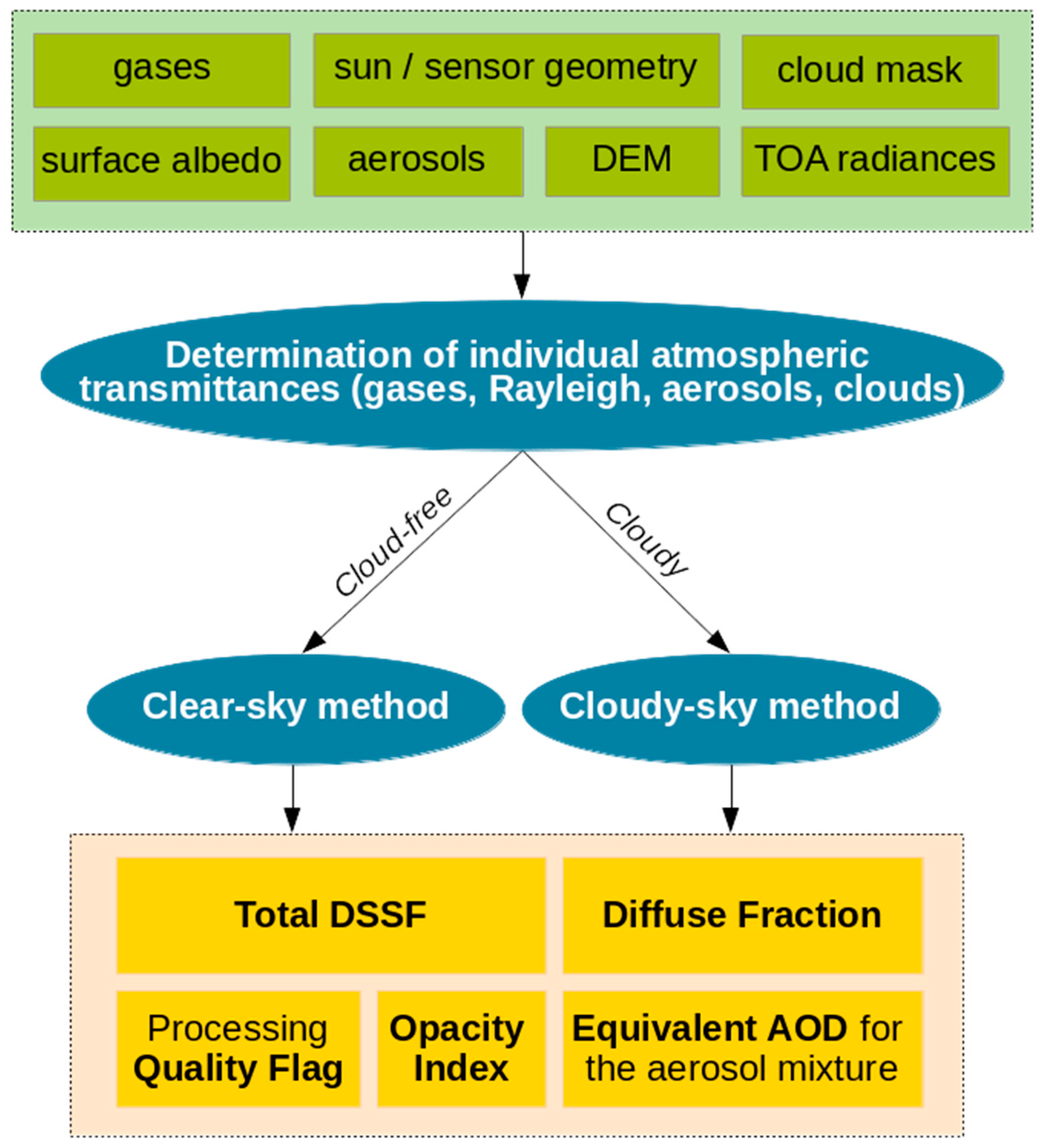
2.2. Overview of the Retrieval Method

An overview of the retrieval method is presented in Figure 1 with a discrimination between the clear and cloudy cases. The list of the retrieved variables is in yellow color. The main two variables are the total DSSF and the diffuse fraction. However, two additional quantities characterizing the atmosphere are also estimated: an equivalent AOD at 550 nm and the Opacity Index. These four variables are all useful to understand the mutual dependencies between them and hence they will all be made available to the user and embedded in the final product (Section 5.1) together with the associated quality flags. Each output estimate is delivered on a pixel-wise basis that propagates the processing quality information of each module (clear-sky and cloudy-sky). The green color is used for the inputs, which will be further explained in Section 3.

The method used for the retrieval of DSSF and $f_d$ is composed of three main steps (see the blue circles in Figure 1): first, the estimations of the individual atmospheric contributions and the total atmospheric transmittance (Section 4.1); second, the parameterization for clear-sky conditions (Section 4.2); and third, the parameterization for cloudy-sky conditions (Section 4.3). The approach chosen for the retrieval is based on explicit physical parameterizations of the contributions of each atmospheric component to the light attenuation. Moreover, the decoupling hypothesis between clear-sky irradiance and cloud attenuation is discussed in reference [44]. Therefore, this first step of the MDSSFTD processing is to determine the transmittance of atmospheric gases, the Rayleigh scattering, the aerosol mixture, and clouds. These individual contributions are then used to estimate the total atmospheric transmittance. A Digital Elevation Model (DEM) is used (see Section 3.2.1) to perform an elevation correction. A discrimination with different parameterizations of the total atmospheric transmittance are therefore used for clear and cloudy pixels. Clear and cloudy pixels are determined through the cloud mask which, therefore, represents an important information. The cloud mask used by MDSSFTD is the satellite derived product described in Section 3.3.1. Despite this clear-sky/cloudy-sky discrimination, a particular attention is paid to ensure the spatial continuity of the radiation estimates at the borders between cloudy-and clear-sky conditions.

3. Input Data

3.1. TOA Data

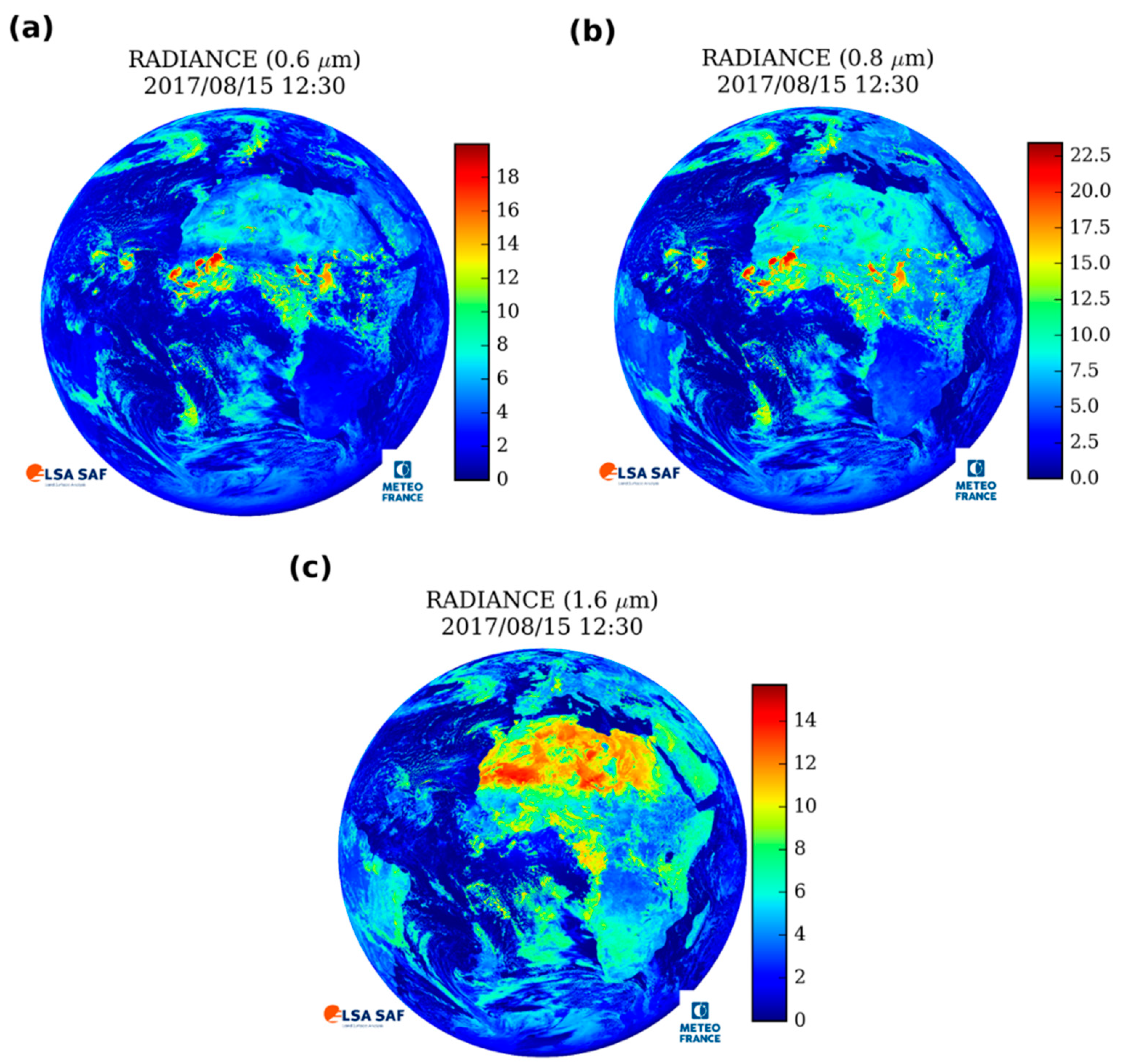
3.1.1. Satellite TOA Radiance

The LSA SAF operational system provides TOA radiances from SEVIRI in the channels centered at 0.6 μm, 0.8 μm, and 1.6 μm (see Figure 2). These data are only used in the cloudy-sky method for the estimation of the cloud albedo and cloud transmittance, as it will be explained in Section 4.1.5. Figure 2 shows the radiation reflected back to space (top-of-atmosphere radiances). The position of clouds for the 15 August 2017 at 12:30 is given in Figure 3. Cloudy areas usually correspond to the areas with highest TOA radiances. It illustrates that the brighter the clouds appear in the satellite images, the more radiation is reflected by them, and therefore the less radiation reaches the ground.

3.1.2. TOA Incoming Sun Radiation

The solar constant used in this algorithm, for both clear-sky and cloudy-sky modules, covers the shortwave band between 0.250 µm and 4 µm, and equals 1367 W/m², as given by the World Meteorological Organization [45]. However, this value will probably need to be adjusted in the next years. The spaceborne radiometers are becoming more and more accurate, and recent measurements seams to yield 1362 Wm⁻² with an uncertainty of order of 2 Wm⁻² [46]. The Sun-Earth distance factor v(t) can be estimated as

$$\begin{array}{c}v\left(t\right)=1.00011+0.034221\times \cos (\Gamma )+0.00128\times \sin (\Gamma )\\ +0.000719\times \cos \left(2\Gamma \right)\\ +0.000077\times \sin \left(2\Gamma \right),\end{array}$$

(9)

with the day angle $\Gamma$ (in radian) defined by reference [47] as $\Gamma =2\Pi \left(k_i-1\right)/365$, $k_i$ being the day of the year.

3.2. Surface Characteristics

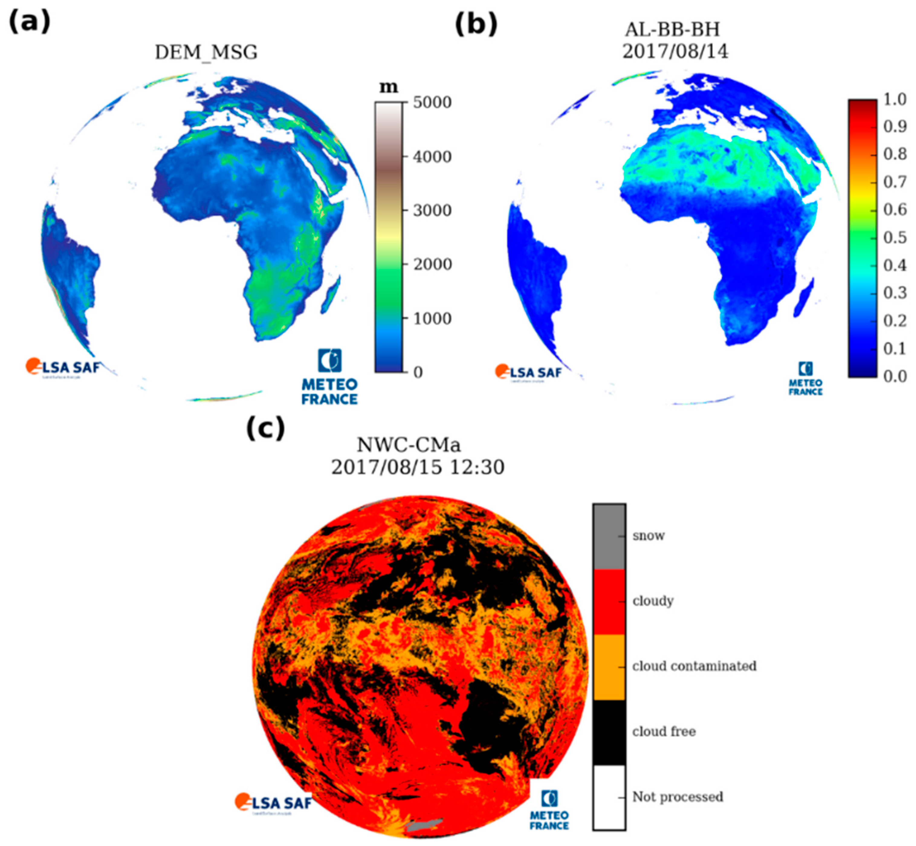
3.2.1. Digital Elevation Models

The MDSSFTD algorithm for clear-sky retrievals relies on two Digital Elevation Model (DEM) files, that are used to correct the aerosol layer height and distribution. The first DEM, noted DEM_MSG, is derived from the USGS GTOPO30 DEM by bilinear interpolation to the SEVIRI grid resolution. The GTOPO30 DEM exploited is originally available at a spatial resolution of 30 arc-seconds (i.e., at approximately 1 km resolution, https://lta.cr.usgs.gov/GTOPO30). This DEM estimates the height at each SEVIRI pixel. The second DEM, noted DEM_CAMS, is the bilinear interpolation to the SEVIRI grid of the coarser DEM used to model the atmospheric fields that are used as input to the MDSSFTD algorithm (see Section 3.3). Figure 3a shows DEM_MSG over the MSG disk.

3.2.2. Land Surface Albedo

The surface albedo used as input for the MDSSFTD algorithm corresponds to the MSG Daily surface Albedo product (MDAL) distributed daily by the LSA SAF in near real time [10,48,49]. The total Broad-Band shortwave Bi-Hemispherical albedo (BB-BH dataset) is chosen as the most appropriate variable to estimate the albedo of the surrounding environment. This ‘environmental’ surface albedo considers the contribution of the area surrounding the processed pixel to the multiple scattering of radiation between the surface and the lower boundary of the atmosphere (indeed, BH offers an integration of directional effects over the target). The MDAL product covers the full MSG disk and is provided at the SEVIRI native spatial resolution. Due to near real time constraints, the albedo of the previous day is used as input of the algorithm. This hypothesis of a stationary albedo is plausible in most of situations. Figure 3b shows the MDAL BB-BH surface albedo for the 14th of August, 2017.

3.3. Atmospheric Characteristics

3.3.1. Cloudiness

Two distinct methods are used to estimate the DSSF, one for clear-sky conditions and one for cloudy-sky conditions (see Section 2.2). The cloud mask used in MDSSFTD is therefore a crucial variable as it allows identifying the cloudiness for all pixels with a high confidence. The absence or presence of clouds for each SEVIRI pixel is derived from the cloud mask that is generated and distributed by the SAF NWC (http://www.nwcsaf.org, reference [50]) to support nowcasting applications. This cloud mask is generated using the operational MSG cloud detection method initially developed by reference [51] and made available every 15 min over the full MSG disk. Figure 3c shows an example of this cloud mask for the 15 August 2017 at 12:30 UTC.

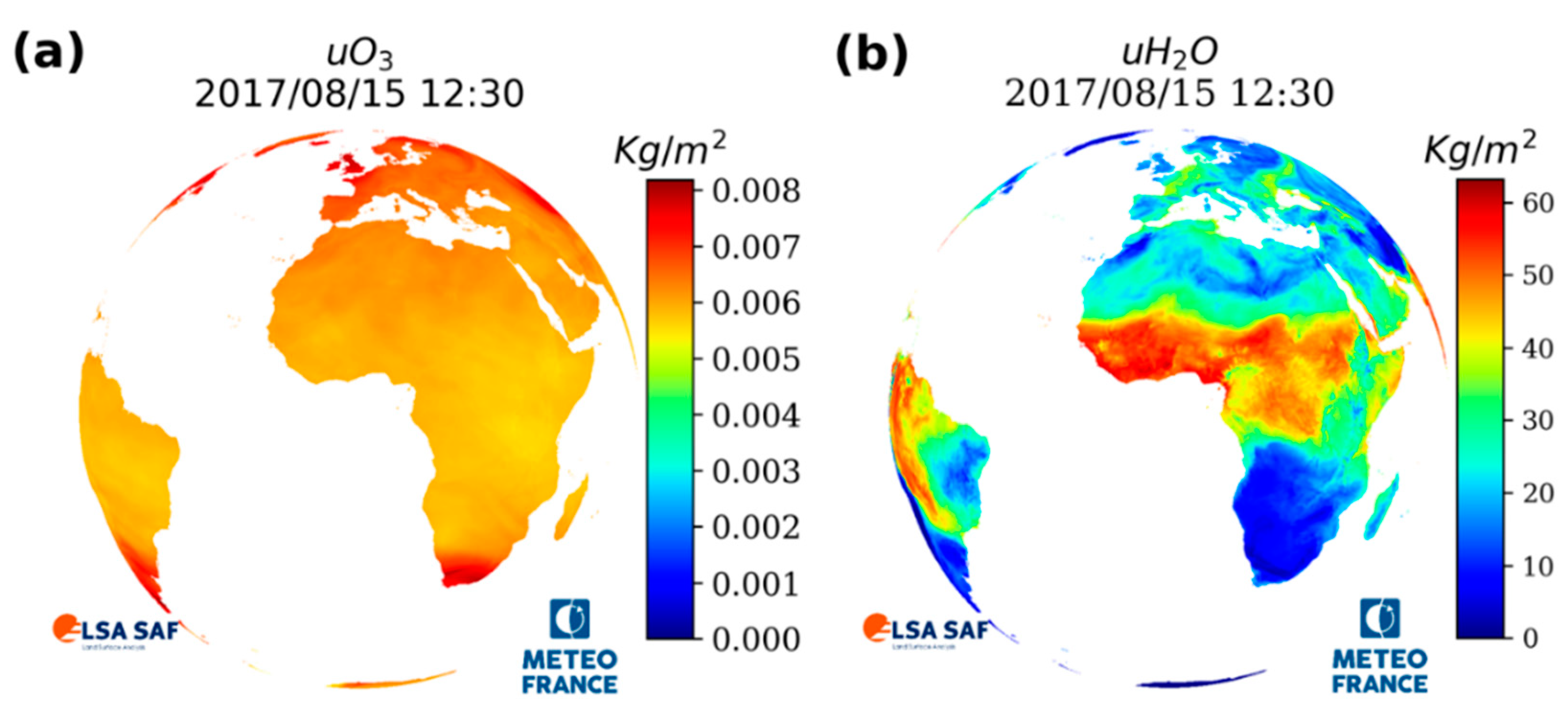
3.3.2. H₂O and O₃ Columnar Content Modeling

The total columnar water vapor ($u_{H_{2}O}$) and total columnar ozone ($u_{O_3}$) content exploited in this study are obtained from the ECMWF Integrated Forecast System (IFS), made available globally with a 0.125° × 0.125° spatial resolution. The operational LSA SAF chain makes use of forecasts up to 36 h ahead available at hourly time-steps. The latest water vapor and ozone forecasts available are then interpolated temporally to a 15-min estimate, and spatially on the MSG disk for ingestion by the MDSSFTD algorithm. Figure 4 gives an overview of $u_{H_{2}O}$ and $u_{O_3}$ fields.

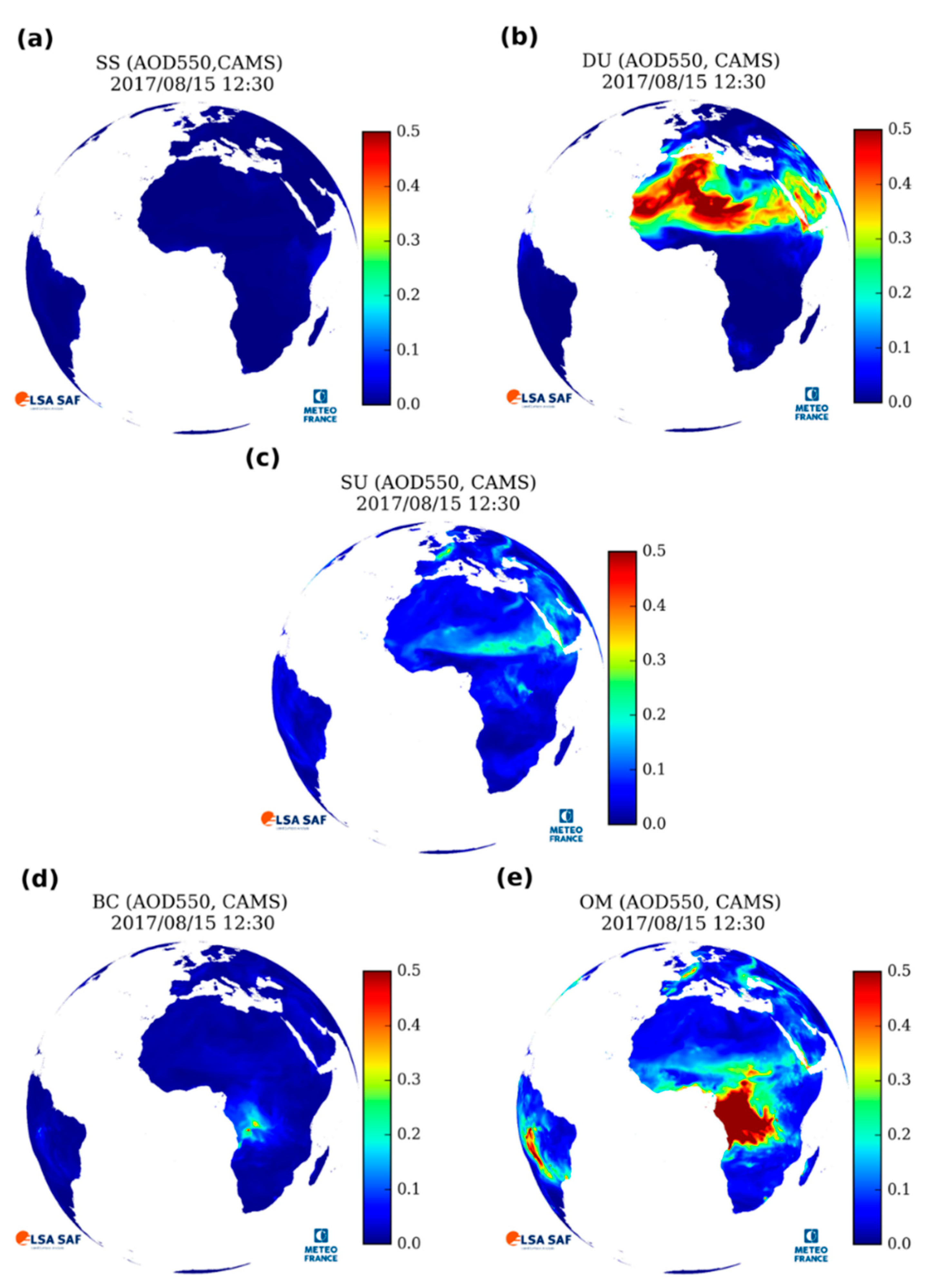
3.3.3. Aerosol Optical Depth and Speciation

The Copernicus Atmosphere Monitoring Service (CAMS, https://atmosphere.copernicus.eu) distributes the aerosol optical depth (AOD) at 550 nm forecasted by the European Centre for Medium-Range Weather Forecasts (ECMWF) for eleven natural and anthropogenic components. Different components are: Sulfate (SU), Sea-Salt (SS), Black Carbon (BC) for 3 classes of particle size, Organic Matter (OM) for 3 classes of particle size, and Dust (DU) for 3 classes of particle size. These aerosols optical depths are available in near-real time and at a spatial resolution of approximately 0.4° × 0.4° (~40 km × 40 km). The delay of a few years between the forecast data and the reanalyses of CAMS is not acceptable in the LSA SAF due to the NRT constraints. Also, CAMS forecasts of AOD are used as input to the MDSSFTD algorithm to constrain the aerosol content and speciation. These aerosol data are interpolated spatially to the MSG/SEVIRI grid. The latest forecast available before the processed timeslot is used (but no longer than 3 h before). Figure 5 gives an overview of the forecast products of aerosol optical depth at 550 nm for all aerosol components modeled for the 15 August 2017 at 12:00 UTC and used as input to the processing of MDSSFTD for the timeslots of the 15 August 2017 from 12:00 UTC to 14:45 UTC.

In order to compute the radiative quantities related to each type of aerosol, we use the Global Aerosol Data Set (GADS) [52], which makes available the optical properties of a number of aerosol types. However, these types do not completely match the CAMS aerosol classification and, therefore, a correspondence between CAMS and GADS aerosol components was implemented, as proposed by reference [53]. At the end, the aerosol layer considered in MDSSFTD is a dynamic mixture of the following aerosol components: the insoluble particles (modeled by the GADS component “INSO”); the water soluble particles (GADS “WASO” component); the black carbon particles (GADS “SOOT” component); the fine and coarse sea-salt particles, referred to as SSALL (combination of GADS classes SSAM and SSCM); and the fine, medium-sized and coarse mineral particles, referred to as MIALL (combination of GADS classes MINM, MIAM and MICM). The properties of the aerosol components used as input of MDSSFTD algorithm are shown in

Table 1. List of the single scattering albedo ($wo$) and hygroscopic nature of the GADS aerosol components, as used by the MDSSFTD algorithm.

	INSO	WASO	SOOT	SSALL	MIALL
Type of particles	Insoluble	Water-soluble	Soot	Sea Salt	Mineral Dust
$wo$ at 500 nm	0.72	0.98	0.23	1.0	0.83
hygroscopic	No	yes	No	Yes	No

.

3.3.4. Aerosol Optical Properties (Look Up Table)

In order to estimate aerosols individual transmittances, the algorithm uses the SIRAMix method (Surface Incident Radiation estimation using Aerosol Mixtures) developed by reference [53]. SIRAMix is based on a physical parameterization of the direct and diffuse DSSF that is fed by a pre-computed Look Up Table (LUT) of aerosol optical properties. The LUT was generated using the radiative transfer model libRadtran [54]. The LUT file is less than 300 kB and allows fast identification of the aerosol optical properties with an optimized computation cost that is well suited for operational purposes. The LUT provides the following variables for each of the 5 GADS aerosol components (INSO, WASO, SOOT, MIALL, SSALL), indexed i in the following and listed in Table 1: (i) the shortwave spherical albedo of aerosols, $A_{aer}^i({\mathsf{\delta }}_0^i,u_{H_{2}O}$) and (ii) the direct and diffuse individual transmittances, $T_{aer,dir}^i\left({\mathsf{\theta }}_s,{\mathsf{\delta }}_0^i,u_{H_{2}O}\right)$ and $T_{aer,dif}^i\left({\mathsf{\theta }}_s,{\mathsf{\delta }}_0^i,u_{H_{2}O}\right)$. The computation of these quantities was made with libRadtran for a predefined range of values for the sun zenith angle (${\mathsf{\theta }}_s$), varying between 0° and 85°; for the total column content of atmospheric water vapor ($u_{H_{2}O}$) (with the corresponding modification of the optical properties of hygroscopic aerosols) varying between 0 and 5 g/cm²; and the aerosol optical depths at 550 nm for each aerosol component i (${\mathsf{\delta }}_0^i$) with values taken between 0 and 4. Interpolation techniques are used to identify the values of these variables for a given atmosphere/geometry combination.

3.4. Summary of the Input Data

Table 2. Summary of the exploitation of each of the input dataset by the processing modules.

Input Category	Input Description and Source	Clear-Sky Method	Cloudy-Sky Method
Atmosphere	MSG SEVIRI TOA radiances	-	X
Geometry	Solar zenith angle (MSG ancillary data)	X	X
Atmosphere	Cloud mask (NWC SAF)	X	X
Atmosphere	GADS aerosols components database [52]	X	X
Atmosphere	Atmospheric forecasts of O3 and H2O gases content from CAMS/ECMWF, interpolated to SEVIRI grid and to 15-min resolution	X	X
Atmosphere	Atmospheric forecasts of AOD per aerosol type, from CAMS/ECMWF, interpolated to SEVIRI grid	X	X
Surface	MSG Shortwave Daily Land Surface Albedos (MDAL, LSA SAF)	X	X
Surface	USGS DEM interpolated to SEVIRI resolution and atmospheric fields DEM interpolated to SEVIRI resolution	X	X
Atmosphere	Aerosol Optical Properties LUT (SIRAMix)	X	X

summarizes the input data sets that are used for the clear-sky and cloud-sky cases. The only difference is the exclusive use of the SEVIRI TOA radiances for the cloudy-sky case.

4. Algorithm Description

4.1. Diffuse and Direct Transmittance Contributions of the Individual Atmospheric Components

4.1.1. Gas Transmittances

The transmittances from gases are used by both methods (clear and cloudy cases) to account for the absorption of gas molecules. They are parametrized empirically according to reference [55] as follows

$$T_{gas, dir, dif}=1-\frac{a\times m^{\prime }\times u_{gas}}{{\left(1+b\times m^{\prime }\times u_{gas}\right)}^c+d\times m^{\prime }\times u_{gas}}$$

(10)

where the sub index gas stands for any of the seven gases mentioned in

Table 3. Coefficients a, b, c, and d used to compute the shortwave gases transmittances; from references [55,56,57,58].

Gases	$\mathit{a}$	$\mathit{b}$	$\mathit{c}$	$\mathit{d}$	${\mathit{u}}_{\mathit{g}\mathit{a}\mathit{s}}(\mathbf{atm}.\mathbf{cm})$
H2O	3.0140	119.300	0.6440	5.8140	Variable (see Section 3.3.2)
O3	0.2554	6107.26	0.2040	0.4710	Variable (see Section 3.3.2)
CO2	0.0721	377.890	0.5855	3.1709	350
CO	0.0062	243.670	0.4246	1.7222	0.075
N2O	0.0326	107.413	0.5501	0.9093	0.28
CH4	0.0192	166.095	0.4221	0.7186	1.60
O2	0.0003	476.934	0.4892	0.1261	2.095 × 105

; the coefficients $a$, $b$, $c$, and $d$ depend on the gas (see Table 3); the pressure-corrected optical air mass ($m^{\prime }$) is described in the following; and $u_{gas}$ corresponds to the total column content for a given gas in units of atm-cm. Here, only the total column water vapor and ozone content are considered as changing variables. These values are derived from the ECMWF forecasts presented in Section 3.3.2, while other $u_{gas}$ values are considered static. Fixed concentrations are given in Table 3. For gases, there is no distinction between direct (‘dir’) and diffuse (‘dif’)—same value of the transmittance is used in both configurations of the radiation.

The pressure corrected air mass ($m^{\prime }$) is defined as:

$$\begin{array}{c}{m}^{\prime }=m(\frac{p}{p_0})\\ \mathrm{with} p=p_0{\left(1-{\mathrm{2.25577.10}}^{-8}\times H_0\right)}^{5.25588}\end{array}$$

(11)

where $p$ is the atmospheric pressure at the surface altitude (in Pa); $p_0$ is the mean atmospheric pressure at sea level ($p_0$ = 101,325 Pa), and $H_0$ is the altitude above sea level (in kilometers); and where $m$ is the optical air mass at standard pressure $p_0$, and is formulated according to reference [59] as:

$$m=\left[\cos ({\theta }_S\right)+0.50572{\left(96.07995-{\theta }_S\right)}^{-1.6364}{]}^{-1}$$

(12)

This equation was found accurate for any air mass up to ${\theta }_s$ < 85° with an error of less than 0.5%.

4.1.2. Rayleigh Direct and Diffuse Transmittances

The total (direct plus diffuse) transmittance due to Rayleigh scattering is formulated according to reference [60] as:

$$T_{Ray,dir+dif}=\exp [-0.1128\times {\left(m^{\prime }\right)}^{0.8346}\times (0.9341-{\left(m^{\prime }\right)}^{0.9868}+0.9391\times m^{\prime })]$$

(13)

where $m^{\prime }$ is the pressure-corrected air mass as defined above in Equations (11) and (12).

The diffuse transmittance due to Rayleigh scattering is formulated according to reference [61] as:

$$T_{Ray,dif}=0.5\times \left(1-T_{Ray, dir+dif}\right)$$

(14)

where the 0.5 factor stands for the forward scattering fraction [62], i.e., the Rayleigh scattering is assumed to be isotropic and only half of the scattered radiation goes downward.

4.1.3. Aerosols Transmittances and Spherical Albedos

The characteristics of each individual aerosol component were presented in Section 3.3.3. The combination of several components results in the aerosol mixtures that are observed in reality. To derive the transmittance and the spherical albedo of the whole aerosol mixture, the individual spectral albedos, and the individual transmittances of each of the aerosol components are determined following reference [53]. These quantities have been pre-computed for different combinations of aerosol load, water vapor and solar zenith angle and used in the SIRAMix as Look Up Table (LUT) for each of the GADS components (see Section 3.3.4). The AOD values from each CAMS aerosol component are converted into AOD values corresponding to the GADS aerosol components. This is done based on the following equations [53]:

$$\begin{array}{c}{\delta }_0^{WASO}={\delta }_0^{SU}+0.5{\delta }_0^{OM}+0.2{\delta }_0^{BC};{\delta }_0^{INSO}=0.5{\delta }_0^{OM};{\delta }_0^{SOOT}=0.8{\delta }_0^{BC};\\ {\delta }_0^{SSALL}={\delta }_0^{SS};{\delta }_0^{MIALL}={\delta }_0^{DU}.\end{array}$$

(15)

The optical depths ${\delta }_0^i$ of the individual aerosol components i are first height-adjusted before being used for the computation of total aerosol transmittance. Indeed, the aerosol layer spreads vertically from the ground ($H_0$) to the top of the aerosol layer ($H_{TOL}$). The CAMS AOD is provided with a ground height ($H_{CAMS})$ defined at its own grid resolution (0.4 degrees), which can differ from the real ground height H₀. Since aerosols are not homogeneously distributed on the vertical, the CAMS AOD converted to GADS types, determined as described in the equation above, may not be adequate to use directly in the computation. Appropriate correction is therefore executed as

$${\delta }_0^{i\_gads, height\_cor}={\delta }_0^{i\_gads}(e^{\frac{-H_0}{Z}}-e^{\frac{-H_{TOL}}{Z}}){(e^{\frac{-H_{0,CAMS}}{Z}}-e^{\frac{-H_{TOL}}{Z}})}^{-1}$$

(16)

where i_GADS stands for the GADS components (INSO, WASO, SOOT, SSALL, MIALL) and Z is the scale height in kilometers. More details on this height correction are given in reference [53]. Values of $Z$ and $H_{TOL}$ are provided for each GADS component in

Table 4. Vertical structure of GADS aerosols as considered in SIRAMix.

GADS Aerosol Components	INSO	WASO	SOOT	SSALL	MIALL
Z (km)	8	8	8	1	2
HTOL (Km)	2	2	2	2	6

.

The equivalent spectral AOD at 550 nm ${\delta }_0^{EQU550}$ is defined as:

$${\delta }_0^{EQU550}={\displaystyle \sum _{i=1}^5}{\delta }_0^{i, height\_cor}$$

(17)

where i index stands for the 5 GADS aerosol components (INSO, WASO, SOOT, SSALL and MIALL), ${\delta }_0^{i,height\_cor}$ the equivalent and height-corrected aerosol optical depth for each aerosol component. This equivalent spectral AOD at 550 nm (Equation (17)) is one of the output variables provided in the MDSSFTD product.

Finally, these spectral AOD at 550 nm are converted to total shortwave (broadband) AOD noted ${\mathsf{\Delta }}_0^i$, as the DSSF is defined based on an integration over a given spectral range. The broadband conversion of the spectral aerosol optical depth of the individual aerosol components is defined as:

$${\mathsf{\Delta }}_0^i=-{\alpha }^i{\left({\delta }_0^i\right)}^2+\beta {\delta }_0^i$$

(18)

where α and β are the regression coefficients determined by radiative transfer simulations for varying aerosol optical depths, as detailed in

Table 5. Regression coefficients for GADS aerosol components to convert spectral AOD into broadband AOD.

GADS Aerosol Components	INSO	WASO	SOOT	SSALL	MIALL
α	0.002	0.057	0.047	0.009	0.002
β	1.022	0.646	0.711	0.961	0.977

.

The broadband spherical albedos and the transmittances can be obtained by extracting the LUT values that correspond to the broadband AOD values for each of the GADS component.

The total aerosol transmittances and total aerosol spherical albedos for the aerosol mixture are determined as the sum of the individual quantities of each component weighted by the corresponding total shortwave AOD ${\mathsf{\Delta }}_0^i$, and normalized by the equivalent broadband AOD (Δ_O), as follows [63]:

$$\begin{array}{c}{T}_{aer,dir}=\frac{1}{{\Delta }_0}{\displaystyle {\sum }_{i=1}^5}{\Delta }_0^i{T}_{aer,dir}^i\\ T_{aer,dif}=\frac{1}{{\Delta }_0}{\displaystyle {\sum }_{i=1}^5}{\Delta }_0^i{T}_{aer,dif}^i\\ A_{aer}=\frac{1}{{\Delta }_0}{\displaystyle {\sum }_{i=1}^5}{\Delta }_0^i{A}_{aer}^i\end{array}$$

(19)

where ${\Delta }_o$ is the equivalent broadband AOD, defined as the summation of the individual broadband aerosol optical depths ${\mathsf{\Delta }}_0^i$ for the 5 components of the aerosol mixture presented above (i.e., INSO, WASO, SOOT, SSALL, and MIALL)

$${\Delta }_0={\displaystyle \sum _{i=1}^5}{\Delta }_0^i$$

(20)

where $i$ index stands for the 5 aerosol components, ${\delta }_0^i$ the equivalent and height-corrected aerosol optical depths for each aerosol component, and ${\alpha }^i$ and ${\beta }^i$ the AOD spectral to broadband conversion coefficients provided in Table 5.

4.1.4. Total Cloud-Free Atmospheric Transmittance

The total cloud-free atmospheric transmittance is equal to the clear-sky transmittance. In cloudy situations, the same value of cloud-free atmospheric transmittance is used for the transmittance happening below the cloud layer. This parameter helps providing an estimation of the total cloudy-case transmittance (Section 4.1.5). Both cloud and cloud-free transmittances and albedos are key parameters for the estimation of the incoming solar radiation at the surface level.

The cloud-free transmittance, $T_{C-freeA}^{}$ is delivered by using the output of SIRAMix module which calculates the clear-sky total DSSF ($E_{tot}^{clear}$, described in reference [53] and briefly discussed in Section 4.2.2):

$$T_{C-freeA}^{}=E_{tot}^{clear}/(E_{0}v\left(t\right)\cos {\theta }_s)=T_{C-freeA}^{ss}(1+\frac{A_S{A}_{C-freeA}^{}}{1-A_S{A}_{C-freeA}^{}}).$$

(21)

This cloud-free atmospheric transmittance $T_{C-freeA}^{}$ is an estimate of the combined effective transmittances of gas absorption, Rayleigh scattering, and aerosol extinction. The parameter $T_{C-freeA}^{}$ is combined with the transmittance of clouds in order to estimate the total DSSF for cloudy-sky case. $T_{C-freeA}$ includes single and multiple scattering contributions between the surface and the albedo of the cloudless atmosphere. One important variable for the cloudy-sky case, which is indirectly estimated here from Equation (21), is the single scattering clear-sky transmittance ($T_{C-freeA}^{ss}$). The two terms in Equation (21) express the product between the single scattering clear-sky transmittance ($T_{C-freeA}^{ss}$) and a multiple scattering factor (in the right hand side of the equation) between the clear-sky atmosphere albedo ($A_{C-freeA}^{}$) and the surface albedo ($A_S$). The albedo of the cloud-free atmosphere is estimated as follows

$$A_{C-freeA}^{}=A_{aer}^{}+A_{Ray},$$

(22)

where $A_{aer}$ is the total broadband aerosol albedo derived from Equation (19), and $A_{Ray}$ is the Rayleigh albedo approximated by reference [64] as a constant value (equal to 0.0685).

4.1.5. Total Cloudy-Sky Atmospheric Transmittance

For cloudy pixels the DSSF is estimated based on a simplified physical description of the radiation interactions in the atmosphere-surface system according to reference [65] and reference [66]. Here it is assumed that a homogeneous cloud layer covers the whole image pixel. The effective transmittance factor $T_{C-A}$ for cloudy atmosphere is therefore given by

$$T_{C-A}=\frac{T_{C-freeA}^{ss}{T}_C}{1-A_S\left(A_{C-freeA}^{}+T_{\mathrm{bc}}{T}_{aer}^2{A}_C\right)}$$

(23)

where $T_{C-freeA}^{ss}$ is the cloud-free single scattering atmospheric transmittance, $T_C$ is the cloud transmittance, $A_S$ is the surface albedo, $T_{\mathrm{bc}}$ is the atmospheric transmittance between the surface and the cloud, and $A_C$ is the cloud albedo of the surrounding pixel approximated by the cloud albedo. The uncertainty due to this approximation can become important in the case of a broken-cloud sky - especially in presence of a dense cloud layer surrounding a partially cloudy contaminated area. The denominator of Equation (23) quantifies the multiple scattering between the surface and the bottom of the cloud layer.

The cloud transmittance $T_C$ and the cloud albedo $A_C$ are key parameters for the estimation of the incoming solar radiation at the surface level. They are highly variable with respect to time and space as they depend on the often-rapid evolution of clouds. The instantaneous values of these two cloud variables are determined from the satellite measurements and with the help of a physical model. The estimation is performed by inverting a system of two equations that approximate the radiative transfer happening within the atmosphere-surface medium including aerosols, gases, and clouds. The approach is an improved version of the one proposed by reference [10]. Because these two cloud variables have broadband characteristics, the satellite spectral reflectances in the spectral channels of the satellite instrument (here the MSG/SEVIRI channels at 0.6 µm, 0.8 µm, and 1.6 µm) are first transformed to broad-band top-of-atmosphere albedo $A_{\mathrm{TOA}}$. We apply the spectral conversion relations proposed by reference [67] based on CERES (Clouds and the Earth’s Radiant Energy System) TOA broadband data and the angular reflectance model of reference [68].

The first equation of the system that is inverted to derive $T_C$ and $A_C$ expresses the albedo at the top of the atmosphere $A_{\mathrm{TOA}}$ as the sum of the different contributions that are illustrated in Figure 6. The TOA albedo depends on (i) radiation coming from Rayleigh scattering of gases above the cloud layer ($A_R$), (ii) radiation reflected by the cloud layer that is attenuated by gases above ($A_c{T}_{SunCloudSat}$), (iii) radiation reflected by the surface that is attenuated by the atmosphere and the cloud layer ($A_s{T}_{SunSurfaceSat}{T}_c^2$), and (iv) radiation reflected by the aerosol layer that is attenuated by the gases and the cloud layer ($A_{aer}{T}_{SunCloudSat}{T}_c^2$):

$$A_{\mathrm{TOA}}=A_R+A_C{T}_{SunCloudSat}+\frac{A_S{T}_{SunSurfaceSat}{T}_C^2}{1-A_S{T}_{\mathrm{bc}}{A}_C}+\frac{A_{aer}{T}_{SunCloudSat}{T}_C^2}{1-A_{aer}{A}_C}$$

(24)

where $T_{\mathrm{bc}}$ is the transmittance below cloud, $T_{SunSurfaceSat}$ is the transmittance between the sun, the surface, and the satellite, and $T_{SunCloudSat}$ is the transmittance between the sun, the cloud, and the satellite. It is important to note that the third term of the equation above accounts for multiple scattering between the surface and the bottom of the cloud layer. Similarly, the fourth term accounts for multiple scattering between the aerosol layer and the cloud layer above it.

The initial parametrizations of $T_{\mathrm{bc}}$ and $T_{SunSurfaceSat}$ (hereafter called $T^{\prime }{}_{\mathrm{bc}}$ and $T^{\prime }{}_{SunSurfaceSat}$) proposed by references [64,65], and also used by reference [10], are only considered as gas transmittances between the cloud and the surface. We improved this parametrization by also considering the influence of aerosols particles by doing $T_{SunSurfaceSat}=T^{\prime }{}_{SunSurfaceSat}\times T_{aer}^2$ and $T_{\mathrm{bc}}=T_{SunSurfaceSat}/T_{SunCloudSat}=T^{\prime }{}_{\mathrm{bc}}\times T_{aer}^2$. In comparison to previous formulation by reference [10], the fourth term in Equation (24) was added for the cloud-aerosol radiative coupling. The new formulation also accounts for the multiple scattering between the top of aerosol layer and the bottom of the cloud layer by using the aerosol albedo. We remember that the MDSSFTD algorithm assumes that aerosols only exist below the cloud layer.

The second equation of the inverted system gives the cloud transmittance $T_C$ expressed in terms of the cloud albedo $A_C$ and the cloud absorption $a_C$ as:

$$T_C=1-A_C-a_C=1-A_C-\alpha A_C.$$

(25)

The cloud absorption is modeled as a linear function of the cloud albedo by introducing the “cloud absorption factor” $\alpha$. The currently employed numerical value of $\alpha =0.11$ was not derived from first principles, but has been adjusted by matching the final flux estimates with the help of a validation database [69]. This parameter therefore mainly serves for “absorbing” the methodological approximations and uncertainties, rather than for quantifying the physical cloud properties. Note that the cloud transmittance $T_C$ could be improved by using a radiative transfer model and taking into account the varying cloud optical thickness as a function of cloud type. Finally, combining the expressions Equation (24) and Equation (25) allows us to calculate the two unknowns $T_C$ and $A_C$ from the “observable” $A_{\mathrm{TOA}}$ by solving a quadratic equation.

The total aerosol transmittance $T_{aer}$ is derived from the total DSSF formula (see Equation (4)) applied to the clear-sky case, as follows

$$T_{aer}=\frac{E_{tot}^{clear}}{\left(E_{0}v\left(t\right)\cos \left({\theta }_s\right)\times T_{H_{2}O}\times T_{O_3}\times T_{mg}\times T_{Ray}\right)}$$

(26)

where the individual transmittances of gases and Rayleigh scattering are defined in Section 4.1.1 and Section 4.1.2.

Finally, the total cloudy-sky atmospheric transmittance is obtained by combining Equation (23) and Equation (21):

$$T_{C-A}=\frac{T_{C-freeA}{T}_C}{1-A_S\times \left(A_{C-freeA}+T_{\mathrm{bc}}{T}_{aer}^2{A}_C\right)}\times \raisebox{1ex}{$1$}\!\left/ \!\raisebox{-1ex}{$\left(1+\frac{A_S{A}_{C-freeA}}{1-A_S{A}_{C-freeA}}\right)$}\right.$$

(27)

where $T_{C-freeA}$ is the cloud-free total atmospheric transmittance.

The previous formulation assures the continuity at the transition between the cloud and cloud-free situations. In the case of no cloud (when $T_C$ = 1 and $A_C$ = 0), $T_{C-A}$ becomes equal to $T_{C-freeA}$, which corresponds to the cloud-free transmittance of the atmosphere.

4.2. Algorithm Description: Clear-Sky Case

4.2.1. Description

In the absence of clouds, the estimation of DSSF is carried out using the method developed by reference [53] referred to as SIRAMix in order to estimate the aerosols individual transmittances. SIRAMix is based on a physical parametrization method coupled with a pre-computed LUT of aerosol properties (see Section 3.3.4) that comprises mainly the direct and diffuse aerosol transmittances of different aerosol components and their corresponding albedos. The input data for aerosol and gaseous components are described in Section 3.3. The originality of SIRAMix is that the effective transmittance of the atmosphere (see Equation (4)) is calculated based upon a combination of the individual transmittances of each gaseous and each aerosol components (i.e., sulfate, soot, sea salt, organic carbon, and mineral dust) with a distinction between direct and diffuse components. The total atmospheric attenuations for direct and diffuse radiation are decomposed into multiple attenuation processes of individual atmospheric direct and diffuse components in order to consider the presence of atmospheric gases ($T_{gases}$), Rayleigh scattering ($T_{Ray}$), and aerosol extinction ($T_{aer}$). This approach is well adapted for the estimation of the diffuse DSSF. The calculation of the total cloud-free transmittance $T_{C-freeA}^{}$ is detailed in Section 4.1.4.

4.2.2. Total DSSF for Clear-Sky Case

The total DSSF, $E_{tot}^{clear}$, reaching the surface under clear-sky conditions is derived with the SIRAMix method as explained above (Section 4.2.1). Its estimation is decomposed in two components: one diffuse, $E_{dif}^{clear}$, and one direct, $E_{dir}^{clear}$, and technically computed as:

$$E_{tot}^{clear}=E_{dir}^{clear}+E_{dif}^{clear}$$

(28)

The diffuse DSSF is also decomposed into two components again: a single scattering term and a multiple scattering term. The estimation of these terms mainly depends on the diffuse transmittance of aerosols ($T_{aer,dif}$; Equation (19)); the diffuse transmittance due to the Rayleigh scattering ($T_{Ray,dif}$; Equation(14)); the shortwave ‘environmental’ albedo of the surrounding surface (see Section 3.2.2); the gas transmittances ($T_{gas}$; see Section 4.1.1); and the albedo of the atmosphere under clear-sky condition (see Section 4.1.4). A more detailed description of the calculation of $E_{tot}^{clear}$ and of its two sub-components ($E_{dif}^{clear}$, $E_{dir}^{clear}$) is given in reference [53]. The most important feature to retain is that the approach is based on the individual transmittance contributions of the different atmospheric components as described above (Section 4.1). In addition, satellite radiances are not directly used here to estimate the incoming solar radiation, but only the sun radiation at the TOA (Section 3.1.2). However, the satellite derived surface albedo is used to retrieve the multi-scattered radiation from the atmosphere to the surface, which could become an important contribution over bright surfaces.

4.2.3. Equivalent AOD, Diffuse Fraction and Opacity Index for Clear-Sky Case

The diffuse fraction at the surface level in clear-sky conditions ($f_D^{clear}$) is derived as follows:

$$f_D^{clear}=\frac{E_{dif}^{clear}}{E_{dif}^{clear}+E_{dir}^{clear}}$$

(29)

This diffuse fraction at the surface level is one of the datasets provided in the MDSSFTD product.

The clearness index $\left(Kt\right)$ is approximated as the amount of the total clear-sky DSSF to the amount of solar flux that is observed at the top of the atmosphere

$$K_t=\frac{E_{total}^{clear}}{E_0\times v\left(t\right)\times \cos {\theta }_s}$$

(30)

The opacity index ($OI$), which is also provided as output of the MDSSFTD product, is derived from Equation (7).

The calculation of the equivalent AOD at 550 nm is detailed in Section 4.1.3 (Equation (17)).

4.3. Algorithm Description: Cloudy-Sky Case

4.3.1. Description

In cloudy conditions, the total DSSF is strongly anti-correlated with the observed reflectance at the TOA. The method for the total DSSF retrieval under cloudy conditions first determines the total shortwave TOA albedo (cloud albedo) and cloud transmittance from the TOA reflectances observed by SEVIRI (Section 3.1.1). Second, the same representation of gases and aerosol contributions than in the clear-sky case is used. Cloud-related terms are determined by inverting a simplified radiative transfer-based model (i.e., the system of two equations described in Section 4.1.5). Finally, the effective transmittance of the cloudy atmosphere, $T_{C-A}$ (Section 4.1.5), is used in Equation (4).

In a different way than the clear-sky method which calculates the diffuse DSSF as a prior step to estimate the diffuse fraction, the cloudy-sky method determines $f_d$ based on the computation of the clearness index ($Kt$). This index was defined by reference [70] and is equal to the overall transmittance $T$ of the atmosphere (see Equation (4)).

4.3.2. Total DSSF in Cloudy Conditions

The total DSSF, $E_{tot}^{cloud}$, in a cloudy situation is determined injecting the total effective transmittance $T_{C-A}$ from Equation (27) in the following equation

$$E_{tot}^{cloud}=E_{0}v\left(t\right)\cos ({\theta }_s)T_{C-A}$$

(31)

where $E_0$ is the solar constant; ${\theta }_s$ the solar zenith angle, $v$(t) is the Sun-Earth distance factor (see Section 3.1.2).

4.3.3. Equivalent AOD, Diffuse Fraction and Opacity Index for Cloudy Case

The diffuse fraction at the surface level in cloudy-sky conditions ($f_D^{cloud}$) is estimated from the total DSSF using the clearness index ($Kt$) as defined in Equation (8). Variable $f_D^{cloud}$ is estimated as proposed by reference [70]:

$$\begin{array}{l}\bullet \hspace{1em}\mathrm{when}{K}_t\le 0.30,\mathrm{then}{f}_D^{cloud}=\left(1.020-0.248K_t\right);\\ \bullet \hspace{1em}\mathrm{when}0.30>K_t<0.78,\mathrm{then}{f}_D^{cloud}=\left(1.450-1.670K_t\right);\\ \bullet \hspace{1em}\mathrm{when} K_t\ge 0.78,\mathrm{then}{f}_D^{cloud}=0.147.\end{array}$$

(32)

To ensure realistic values, the diffuse fraction is set to a value of 1 when the cloud transmittance is zero (i.e., in the presence of very bright clouds). When the cloud transmittance is one (e.g., clear-sky situation incorrectly flagged as cloudy by the input cloud mask), then the clear-sky method is used. The case when $K_t\ge 0.78$ is quite uncommon and only occurs in case of very thin clouds and pure atmosphere with low quantities of atmospheric particles and gas (or false cloud detections). This empirical method was chosen as it was validated over a number of sites in Europe. Reference [71] reviewed a number of direct/diffuse irradiance separation methods. Many of them were complex methods with several predictors which proved good efficiency. However, these methods were developed for high-frequency irradiance data, or they rely on future state estimators so that they are not implementable in near-real time nor with 15-min instantaneous satellite measurements like SEVIRI. The methods developed by reference [26] or reference [72] also seem powerful with a low degree of complexity. The impact of such methods is planned to be further analyzed for the case of our MSG data in the future in the framework of the evolution of the MDSSFTD product.

The estimation of the opacity index ($OI$) of the total column of the atmosphere remains unchanged compared to the clear-sky case (Equation (7)).

The calculation of the equivalent AOD at 550 nm is strictly identical under clear-sky and cloudy-sky conditions and detailed in Section 4.1.3.

5. Results

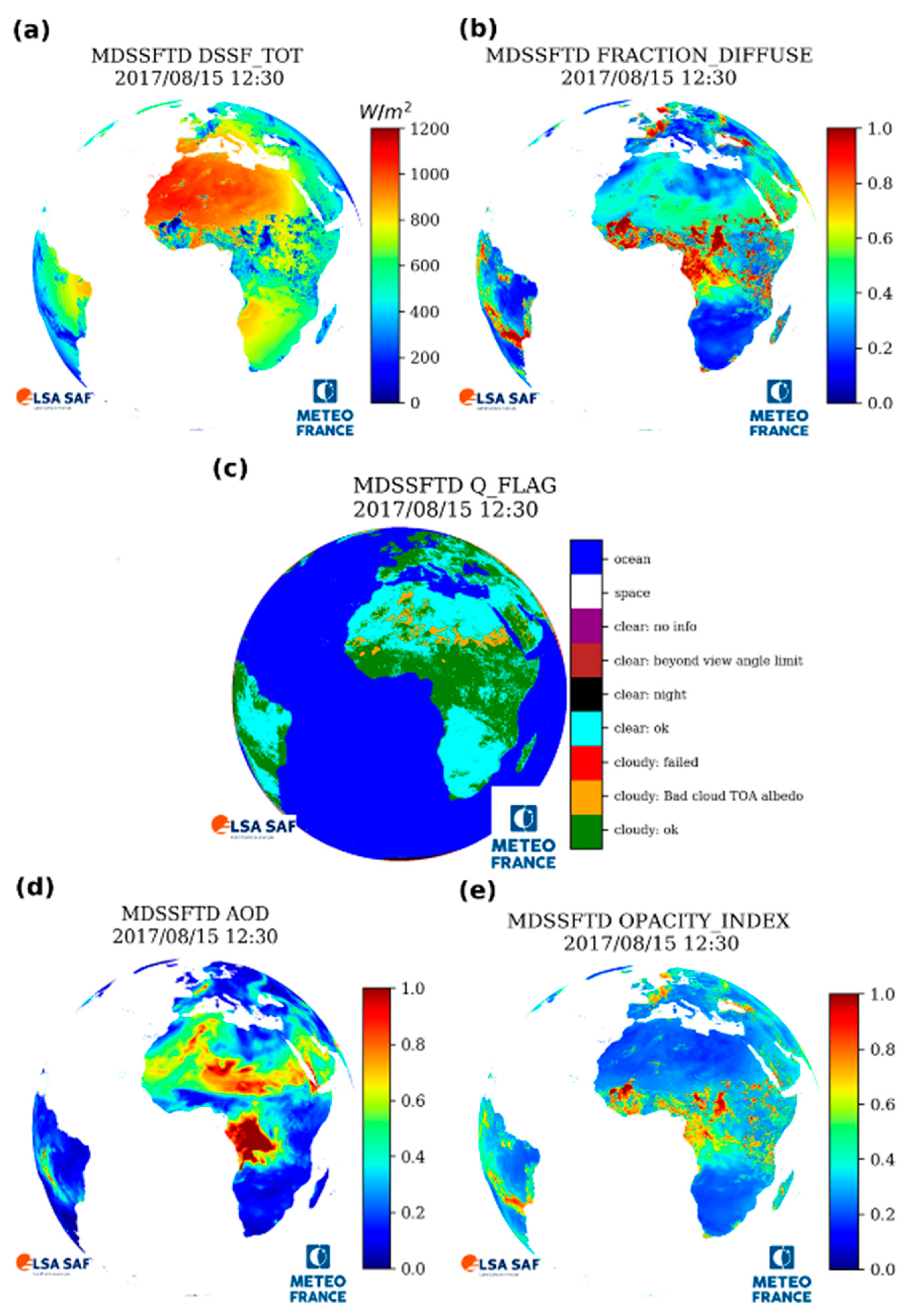
5.1. Overview of the Output Variables

Figure 7 shows an example of MDSSFTD product for the 15th of August, 2017 at 12:30 UTC, as generated by the operational processing chain of the LSA SAF. The output comprises the following datasets:

• total DSSF, named ‘DSSF_TOT’ in the MDSSFTD product;
• diffuse DSSF fraction, named ‘FRACTION_DIFFUSE’;
• equivalent spectral AOD at 550 nm for the current aerosol load, named ‘AOD’;
• the opacity of the atmosphere, named ‘OPACITY_INDEX’;
• processing quality flags, named ‘Q_FLAG’.

As it can be seen in Figure 7, the total DSSF decreases over the areas that are cloudy, whereas the diffuse fraction increases over these regions. However, diffuse fraction can also increase with the AOD (see in North Africa over the Sahara Desert due to dust and in Southern Africa over Angola and Congo due to biomass-burning aerosols).

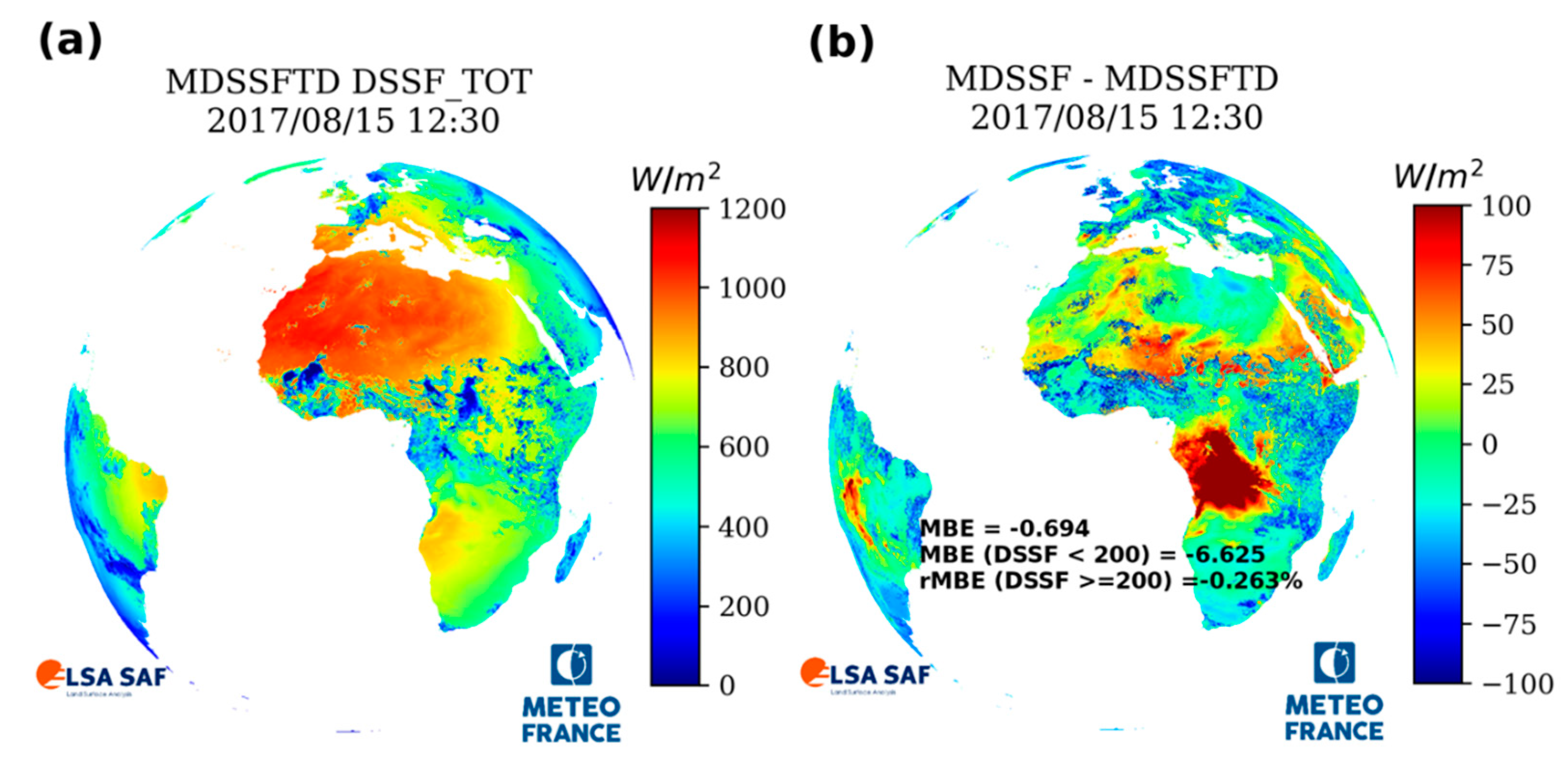
5.2. Comparison with the Previous LSA SAF DSSF Product Version

The MDSSFTD method differs from the MDSSF method (from reference [10] and currently used for the operational production of DSSF) in several aspects such as the parametrization of gaseous transmittances and the aerosol contribution. The only case when the two algorithms would give similar results would be under clear-sky conditions when MDSSFTD aerosol inputs are equivalent to a horizontal visibility of 20 km corresponding to continental aerosols, which is the constant aerosol conditions set in the MDSSF algorithm. In the cloudy-sky case, the main difference lies in the impact of the aerosol layer below the cloud layer that is now considered in the MDSSFTD product. Figure 8 presents the difference of the total solar flux measurements from the two LSA SAF satellite-derived product versions (ref. LSA-201 and LSA-207 for MDSSF and MDSSFTD, respectively) for a particular day and time slot (15 August 2017 at 12:30 UTC). The spatial differences between the two estimates of the DSSF are many. For example, the area with the maximal difference between the two products is located in Central Africa (see red-coloured values on Figure 8), with values above 100 W/m² over Angola/Republic of Congo. This is due to the important amount of aerosols in the atmosphere over this region and for this period of the year (see equivalent AOD in Figure 7d), resulting from biomass burning (see Figure 5). The strong influence of aerosols is considered for the estimation of MDSSFTD total flux, while it is not the case for MDSSF. Moreover, Figure 7c shows that this region is cloudy, which contributes to increase the differences. Consequently, this is an interesting case that illustrates the major importance of considering the attenuation of the radiation due to aerosols not only in clear-sky conditions. A more detailed comparison between the operational MDSSF product and the upcoming MDSSFTD will be given in the companion article [73].

5.3. Known Issues and Limitations

The MDSSFTD product for clear-sky conditions has been updated compared to the previous operational method (MDSSF). The main evolution is the consideration of the presence of dynamic aerosol conditions and the delivery of diffuse fraction estimates. The first limitation is that the current version of the algorithm depends on the quality of the aerosol inputs. The uncertainty associated to the AOD coming from CAMS is the major source of error for the estimate of DSSF and for the diffuse fraction under clear sky conditions. Reference [53] showed that clear-sky retrievals of DSSF are accurate enough for CAMS reanalysis dataset but of much lower quality when using the forecast products as input to the processing.

The accuracy of the MDSSFTD product also depends on the uncertainty introduced by the dependencies on the surface albedo and on the approximations for the calculation of TOA albedo from the SEVIRI spectral radiances. For example, in the presence of snow, the satellite values of surface albedo are often less accurate. This will affect the accuracy of the estimated DSSF, as surface albedo helps to estimate the multiple scattering of radiation between the surface and the atmosphere. Furthermore, multiple scattering can be very important in the presence of snow, which corresponds to a high value of albedo.

The cloud mask also represents a highly sensitive auxiliary input data. Missing cloud detections can significantly impact the product quality. Also, we know that the presence of broken clouds (i.e., clouds not covering a whole SEVIRI pixel) are not properly considered by the model (nor the cloud mask), which assumes a homogeneous cloud layer over the whole pixel [74]. MDSSFTD results on SEVIRI pixels switching in time from clear to cloudy conditions or reciprocally, from cloudy to clear, are very likely to correspond to conditions of broken clouds, and therefore shall be considered with caution by the users.

A limitation could be also found due to the underestimation of the multi-scattering processes in the case of a recent snow-fall that could therefore not be considered yet by using as input the yesterday’s LSA SAF satellite surface albedos.

Finally, a restriction is applied in the look-up-table for aerosol properties to sun zenith angles smaller than 85 degrees. This is required as the radiative transfer model, and the MDSSFTD algorithm itself, are not well suited for extreme zenith angles. In conclusion, this restriction disables the data availability under twilight conditions (${\theta }_s$ > 85 degrees). For the MSG/SEVIRI platform, this occurs in wintertime over high latitude regions.

5.4. Access to the Code Sources and Data Policy

The MDSSFTD code is made available in open source under the CeCILL-C license. Users shall therefore follow the principles of this license and, in particular, the rules for the exploitation of the code. In addition, users are kindly requested to duly acknowledge authors of the code: “The MDSSFTD code (Carrer et al., 2019a, b) was made available to the community by CNRM/Météo-France thanks to the support of EUMETSAT.”

The code is accessible at the following location: https://opensource.umr-cnrm.fr/projects/mdssftd.

6. Conclusions

This article presents a method for the estimation of the total DSSF and the corresponding diffuse fraction for both clear-sky and cloudy-sky situations observed by the SEVIRI instrument aboard the MSG satellite. The method first determines the individual contributions of clouds, gases and aerosols. Second, two specific retrieval modules based on physical parameterizations are used to estimate the DSSF and the diffuse fraction for clear-sky and cloudy-sky situations. The code corresponding to the scientific algorithm is made available to the community. The algorithm is today implemented in the LSA SAF chain and the associated MDSSFTD product is available to the community since July 2019; back-processing may also be requested. The LSA SAF dissemination methods are described in reference [49]. The validation of the method presented in this article is reported in the companion paper [73]. The evaluation was conducted by comparing the instantaneously retrieved total DSSF and diffuse fraction (fd) against ground measurements and other satellite-based products. For all sky conditions, total DSSF obtained an average MBE of 3.6 W m⁻² and rMBE of 0.3% when compared to in situ measurements, whereas MBE and rMBE for the diffuse fraction were found to be, respectively, −0.04% and −17.7%. Furthermore, the MDSSFTD product showed a good agreement when compared to other radiation products such as the one from CAMS and the original MDSSF product from the LSA SAF. Finally, it is important to notice that although the LSA SAF was initially designed to serve the needs of the meteorological community, there is no doubt that this MDSSFTD product can address a much broader set of applications, which includes users from the agricultural and forestry sectors, as well as from the renewable energy industry.

References

1. Ramanathan, V.; Cess, R.D.; Harrison, E.F.; Minnis, P.; Barkstrom, B.R.; Ahmad, E.; Hartmann, D. Cloud-Radiative Forcing and Climate: Results from the Earth Radiation Budget Experiment. Science 1989, 243, 57–63. [Google Scholar] [CrossRef] [PubMed] [Green Version]
2. Dickinson, R.E. Land surface processes and climate–Surface albedos and energy balance. Adv. Geophys. 1983, 25, 305–353. [Google Scholar]
3. Mitchell, K.E.; Lohmann, D.; Houser, P.R.; Wood, E.F.; Schaake, J.C.; Robock, A.; Cosgrove, B.A.; Sheffield, J.; Duan, Q.; Luo, L.; et al. The multi-institution North American Land Data Assimilation System (NLDAS): Utilizing multiple GCIP products and partners in a continental distributed hydrological modeling system. J. Geophys. Res. Space Phys. 2004, 109, D7. [Google Scholar] [CrossRef]
4. Ferranti, L.; Viterbo, P. The European Summer of 2003: Sensitivity of Soil Water Initial Conditions. J. Clim. 2006, 19, 3659–3680. [Google Scholar] [CrossRef]
5. Carrer, D.; Lafont, S.; Roujean, J.-L.; Calvet, J.-C.; Meurey, C.; Le Moigne, P.; Trigo, I.F.; Trigo, I. Incoming Solar and Infrared Radiation Derived from METEOSAT: Impact on the Modeled Land Water and Energy Budget over France. J. Hydrometeorol. 2012, 13, 504–520. [Google Scholar] [CrossRef]
6. Carrer, D.; Roujean, J.-L.; Lafont, S.; Calvet, J.-C.; Boone, A.; Decharme, B.; Delire, C.; Gastellu-Etchegorry, J.-P.; Gastellu-Etchegorry, J. A canopy radiative transfer scheme with explicit FAPAR for the interactive vegetation model ISBA-A-gs: Impact on carbon fluxes. J. Geophys. Res. Biogeosciences 2013, 118, 888–903. [Google Scholar] [CrossRef] [Green Version]
7. Mercado, L.M.; Bellouin, N.; Sitch, S.; Boucher, O.; Huntingford, C.; Wild, M.; Cox, P.M. Impact of changes in diffuse radiation on the global land carbon sink. Nature 2009, 458, 1014. [Google Scholar] [CrossRef]
8. O’Sullivan, M.; Rap, A.; Reddington, C.L.; Spracklen, D.V.; Gloor, M.; Buermann, W. Small global effect on terrestrial net primary production due to increased fossil fuel aerosol emissions from East Asia since the turn of the century. Geophys. Res. Lett. 2016, 43, 8060–8067. [Google Scholar] [CrossRef]
9. Blanc, P.; Espinar, B.; Geuder, N.; Gueymard, C.; Meyer, R.; Pitz-Paal, R.; Reinhardt, B.; Renné, D.; Sengupta, M.; Wald, L.; et al. Direct normal irradiance related definitions and applications: The circumsolar issue. Sol. Energy 2014, 110, 561–577. [Google Scholar] [CrossRef]
10. Geiger, B.; Meurey, C.; Lajas, D.; Franchisteguy, L.; Carrer, D.; Roujean, J.-L. Near real-time provision of downwelling shortwave radiation estimates derived from satellite observations. Meteorol. Appl. 2008, 15, 411–420. [Google Scholar] [CrossRef]
11. Bishop, J.K.B.; Rossow, W.B. Spatial and temporal variability of global surface solar irradiance. J. Geophys. Res. Space Phys. 1991, 96, 16839–16858. [Google Scholar] [CrossRef]
12. Darnell, W.L.; Staylor, W.F.; Gupta, S.K.; Denn, F.M. Estimation of Surface Insolation Using Sun-Synchronous Satellite Data. J. Clim. 1988, 1, 820–835. [Google Scholar] [CrossRef]
13. Dedieu, G.P.; Deschamps, P.; Kerr, Y. Satellite estimation of solar irradiance at the surface of the earth and of surface albedo using a physical model applied to METEOSAT data. J. Clim. Appl. Meteorol. 1987, 26, 79–87. [Google Scholar] [CrossRef]
14. Gautier, C.; Landsfeld, M. Surface Solar Radiation Flux and Cloud Radiative Forcing for the Atmospheric Radiation Measurement (ARM) Southern Great Plains (SGP): A Satellite, Surface Observations, and Radiative Transfer Model Study. J. Atmos. Sci. 1997, 54, 1289–1307. [Google Scholar] [CrossRef]
15. Cano, D.; Monget, J.; Albuisson, M.; Guillard, H.; Regas, N.; Wald, L. A method for the determination of the global solar radiation from meteorological satellite data. Sol. Energy 1986, 37, 31–39. [Google Scholar] [CrossRef] [Green Version]
16. Li, Z.; Leighton, H.G. Global climatologies of the solar radiation budgets at the surface and in the atmosphere from 5 years of ERBE data. J. Geophys. Res. 1993, 98, 4919–4930. [Google Scholar] [CrossRef]
17. Masuda, K.; Leighton, H.G.; Li, Z. A New Parameterization for the Determination of Solar Flux Absorbed at the Surface from Satellite Measurements. J. Clim. 1995, 8, 1615–1629. [Google Scholar] [CrossRef]
18. Moser, W.; Raschke, E. Incident Solar Radiation over Europe Estimated from METEOSAT Data. J. Clim. Appl. Meteorol. 1984, 23, 166–170. [Google Scholar] [CrossRef] [Green Version]
19. Pinker, R.T.; Ewing, J.A. Modeling Surface Solar Radiation: Model Formulation and Validation. J. Clim. Appl. Meteorol. 1985, 24, 389–401. [Google Scholar] [CrossRef] [Green Version]
20. Pinker, R.T.; Laszlo, I. Modeling Surface Solar Irradiance for Satellite Applications on a Global Scale. J. Appl. Meteorol. 1992, 31, 194–211. [Google Scholar] [CrossRef] [Green Version]
21. Tarpley, J.D. Estimating Incident Solar Radiation at the Surface from Geostationary Satellite Data. J. Appl. Meteorol. 1979, 18, 1172–1181. [Google Scholar] [CrossRef] [Green Version]
22. Whitlock, C.H.; Charlock, T.P.; Staylor, W.F.; Pinker, R.T.; Laszlo, I.; Ohmura, A.; Gilgen, H.; Konzelman, T.; DiPasquale, R.C.; Moats, C.D.; et al. First Global WCRP Shortwave Surface Radiation Budget Dataset. Bull. Am. Meteorol. Soc. 1995, 76, 905–922. [Google Scholar] [CrossRef] [Green Version]
23. Romano, F.; Cimini, D.; Cersosimo, A.; Di Paola, F.; Gallucci, D.; Gentile, S.; Geraldi, E.; LaRosa, S.; Nilo, S.T.; Ricciardelli, E.; et al. Improvement in Surface Solar Irradiance Estimation Using HRV/MSG Data. Remote Sens. 2018, 10, 1288. [Google Scholar] [CrossRef]
24. Gallucci, D.; Romano, F.; Cersosimo, A.; Cimini, D.; Di Paola, F.; Gentile, S.; Geraldi, E.; LaRosa, S.; Nilo, S.T.; Ricciardelli, E.; et al. Nowcasting Surface Solar Irradiance with AMESIS via Motion Vector Fields of MSG-SEVIRI Data. Remote. Sens. 2018, 10, 845. [Google Scholar] [CrossRef]
25. Ineichen, P. High Turbidity Solis Clear Sky Model: Development and Validation. Remote Sens. 2018, 10, 435. [Google Scholar] [CrossRef]
26. Ruiz-Arias, J.A.; Alsamamra, H.; Tovar-Pescador, J.; Pozo-Vazquez, D. Proposal of a regressive model for the hourly diffuse solar radiation under all sky conditions. Energy Convers. Manag. 2010, 51, 881–893. [Google Scholar] [CrossRef]
27. Rigollier, C.; Lefèvre, M.; Wald, L. The method Heliosat-2 for deriving shortwave solar radiation from satellite images. Sol. Energy 2004, 77, 159–169. [Google Scholar] [CrossRef] [Green Version]
28. Ineichen, P. Long Term HelioClim-3 Global, Beam and Diffuse Irradiance Validation. 2016. Available online: https://archive-ouverte.unige.ch/unige:81915/ (accessed on 26 June 2019).
29. Trigo, I.F.; DaCamara, C.C.; Viterbo, P.; Roujean, J.L.; Olesen, F.; Barroso, C.; Camacho-de-Coca, F.; Carrer, D.; Freitas, S.C.; García-Haro, J.; et al. The Satellite Application Facility on Land Surface Analysis. Int. J. Remote Sens. 2011, 32, 2725–2744. [Google Scholar] [CrossRef]
30. Schmetz, J.; Pili, P.; Tjemkes, S.; Just, D.; Kerkmann, J.; Rota, S.; Ratier, A. An Introduction to Meteosat Second Generation (MSG). Bull. Am. Meteorol. Soc. 2002, 83, 977–992. [Google Scholar] [CrossRef]
31. Ineichen, P.; Barroso, C.S.; Geiger, B.; Hollmann, R.; Marsouin, A.; Mueller, R. Satellite Application Facilities irradiance products: hourly time step comparison and validation over Europe. Int. J. Remote Sens. 2009, 30, 5549–5571. [Google Scholar] [CrossRef]
32. Roerink, G.; Bojanowski, J.; De Wit, A.; Eerens, H.; Supit, I.; Leo, O.; Boogaard, H. Evaluation of MSG-derived global radiation estimates for application in a regional crop model. Agric. For. Meteorol. 2012, 160, 36–47. [Google Scholar] [CrossRef]
33. Moreno, A.; Gilabert, M.; Camacho, F.; Martínez, B. Validation of daily global solar irradiation images from MSG over Spain, Renew. Energy 2013, 60, 332–342. [Google Scholar]
34. Bevan, S.L.; North, P.R.; Los, S.O.; Grey, W.M. A global dataset of atmospheric aerosol optical depth and surface reflectance from AATSR. Remote Sens. Environ. 2012, 116, 199–210. [Google Scholar] [CrossRef]
35. Lubin, D.; Woodbridge, E.; Collins, W.; Zalpuri, K.S.; Jayaraman, A.; Ramachandran, S.; Ramanathan, V.; Collins, W.D. Direct observations of aerosol radiative forcing over the tropical Indian Ocean during the January-February 1996 pre-INDOEX cruise. J. Geophys. Res. Space Phys. 1998, 103, 13827–13836. [Google Scholar]
36. Satheesh, S.K.; Ramanathan, V. Large differences in tropical aerosol forcing at the top of the atmosphere and Earth’s surface. Nature 2000, 405, 60–63. [Google Scholar] [CrossRef]
37. Cherian, R.; Quaas, J.; Salzmann, M.; Wild, M. Pollution trends over Europe constrain global aerosol forcing as simulated by climate models. Geophys. Res. Lett. 2014, 41, 2176–2181. [Google Scholar] [CrossRef] [Green Version]
38. Drame, M.S.; Ceamanos, X.; Roujean, J.L.; Boone, A.; Lafore, J.P.; Carrer, D.; Geoffroy, O. On the Importance of Aerosol Composition for Estimating Incoming Solar Radiation: Focus on the Western African Stations of Dakar and Niamey during the Dry Season. Atmosphere 2015, 6, 1608–1632. [Google Scholar] [CrossRef] [Green Version]
39. Gelaro, R.; McCarty, W.; Suárez, M.J.; Todling, R.; Molod, A.; Takacs, L.; Wargan, K. The Modern-Era Retrospective Analysis for Research and Applications, Version 2 (MERRA-2). J. Clim. 2017, 30, 5419–5454. [Google Scholar] [CrossRef]
40. Rémy, S.; Kipling, Z.; Flemming, J.; Boucher, O.; Nabat, P.; Michou, M.; Bozzo, A.; Ades, M.; Huijnen, V.; Benedetti, A.; et al. Description and evaluation of the tropospheric aerosol scheme in the Integrated Forecasting System (IFS-AER, cycle 45R1) of ECMWF. Geosci. Model Dev. Discuss. 2019. [Google Scholar] [CrossRef]
41. Chan, K.L.; Wiegner, M.; Flentje, H.; Mattis, I.; Wagner, F.; Gasteiger, J.; Geiß, A. Evaluation of ECMWF-IFS (version 41R1) operational model forecasts of aerosol transport by using ceilometer network measurements. Geosci. Model Dev. 2018, 11, 3807–3831. [Google Scholar] [CrossRef] [Green Version]
42. Carrer, D.; Ceamanos, X.; Six, B.; Roujean, J.-L. AERUS-GEO: A newly available satellite-derived aerosol optical depth product over Europe and Africa. Geophys. Res. Lett. 2014, 41, 7731–7738. [Google Scholar] [CrossRef]
43. Xu, H.; Ceamanos, X.; Roujean, J.-L.; Carrer, D.; Xue, Y. Can satellite-derived aerosol optical depth quantify the surface aerosol radiative forcing? Atmos. Res. 2014, 150, 151–167. [Google Scholar] [CrossRef]
44. Oumbe, A.; Qu, Z.; Blanc, P.; Lefèvre, M.; Wald, L.; Cros, S. Decoupling the effects of clear atmosphere and clouds to simplify calculations of the broadband solar irradiance at ground level. Geosci. Model Dev. 2014, 7, 1661–1669. [Google Scholar] [CrossRef] [Green Version]
45. World Meteorological Organization (WMO). Measurement of sunshine duration. In WMO-No. 8–Guide to Meteorological Instruments and Methods of Observation; WMO: Geneva, Switzerland, 2006. [Google Scholar]
46. Meftah, M.; Dewitte, S.; Irbah, A.; Chevalier, A.; Conscience, C.; Crommelynck, D.; Janssen, E.; Mekaoui, S. SOVAP/Picard, a spaceborne Radiometer to Measure the Total Solar Irradiance. Sol. Phys. 2014, 289, 1885–1899. [Google Scholar] [CrossRef]
47. Spencer, J.W. Fourier series representation of the position of the sun. Search 1971, 2, 172. [Google Scholar]
48. Carrer, D.; Roujean, J.-L.; Meurey, C. Comparing operational MSG/SEVIRI land surface albedo products from Land SAF with ground measurements and MODIS. IEEE Trans. Geosci. Remote Sens. 2010, 48, 1714–1728. [Google Scholar] [CrossRef]
49. Carrer, D.; Moparthy, S.; Lellouch, G.; Ceamanos, X.; Pinault, F.; Freitas, S.C.; Trigo, I.F. Land Surface Albedo Derived on a Ten Daily Basis from Meteosat Second Generation Observations: The NRT and Climate Data Record Collections from the EUMETSAT LSA SAF. Remote Sens. 2018, 10, 1262. [Google Scholar] [CrossRef]
50. NWC SAF. User Manual for the Cma, CT, CTTH, CMIC Products of NWC SAF/GEO: Scientific Part, version v2016; NWC SAF, 2016; Available online: http://www.nwcsaf.org/Downloads/GEO/2018/Documents/Scientific_Docs/NWC-CDOP3-GEO-MF-CMS-SCI-UM-Cloud_v1.0.pdf (accessed on 28 October 2019).
51. Derrien, M.; Le Gléau, H. MSG/SEVIRI cloud mask and type from SAFNWC. Int. J. Remote Sens. 2005, 26, 4707–4732. [Google Scholar] [CrossRef]
52. Koepke, P.; Hess, M.; Schult, I.; Shettle, E.P. Global Aerosol Data Set; Tech. Rep. 243; Max-Planck-Institut für Meteorologie: Hamburg, Germany, 1997. [Google Scholar]
53. Ceamanos, X.; Carrer, D.; Roujean, J.-L. Improved retrieval of direct and diffuse downwelling surface shortwave flux in cloudless atmosphere using dynamic estimates of aerosol content and type: application to the LSA-SAF project. Atmos. Chem. Phys. Discuss. 2014, 14, 8209–8232. [Google Scholar] [CrossRef] [Green Version]
54. Mayer, B.; Kylling, A. Technical note: The libRadtran software package for radiative transfer calculations – description and examples of use. Atmos. Chem. Phys. 2005, 5, 1855–1877. [Google Scholar] [CrossRef]
55. Psiloglou, B.E.; Kambezidis, H.D. Performance of the mete-orological radiation model during the solar eclipse of 29 March 2006. Atmos. Chem. Phys. 2007, 7, 6047–6059. [Google Scholar] [CrossRef]
56. Kambezidis, H.D. Current Trends in Solar Radiation Modeling: The Paradigm of MRM. J. Fundam. Renew. Energy Appl. 2016, 6, e106. [Google Scholar] [CrossRef]
57. Kambezidis, H.D.; Psiloglou, B.E.; Karagiannis, D.; Dumka, U.C.; Kaskaoutis, D.G. Meteorological radiation model (mrm v6.1): Improvements in diffuse radiation estimates and a new approach for implementation of cloud products. Renew. Sustain. Energy Rev. 2017, 74, 616–637. [Google Scholar] [CrossRef]
58. Psiloglou, B.E.; Santamouris, M.; Asimakopoulos, D.N. Predicting the broadband transmittance of the uniformly mixed gases (CO2, CO, N2O, CH4 and O2) in the atmosphere, for solar radiation models. Renew. Energy 1995, 6, 63–70. [Google Scholar] [CrossRef]
59. Kasten, F.; Young, A.T. Revised optical air mass tables and approximation formula. Appl. Opt. 1989, 28, 4735–4738. [Google Scholar] [CrossRef]
60. Psiloglou, B.E.; Santamouris, M.; Asimakopoulos, D.N. On broadband Rayleigh scattering in the atmosphere for solar radiation modelling. Renew. Energy 1995, 6, 429–433. [Google Scholar] [CrossRef]
61. Bird, R.E.; Hulstrom, R.L. Simplified Clear Sky Model for Direct and Diffuse Insolation on Horizontal Surfaces (No. SERI/TR-642-761); Solar Energy Research Inst.: Golden, CO, USA, 1981. [Google Scholar]
62. Mengüç, M.P.; Viskanta, R. Comparison of radiative transfer approximations for a highly forward scattering planar medium. J. Quant. Spectrosc. Radiat. Transf. 1983, 29, 381–394. [Google Scholar] [CrossRef]
63. Ceamanos, X.; Carrer, D.; Roujean, J.-L. An efficient approach to estimate the transmittance and reflectance of a mixture of aerosol components. Atmos. Res. 2014, 137, 125–135. [Google Scholar] [CrossRef]
64. Lacis, A.A.; Hansen, J. A Parameterization for the Absorption of Solar Radiation in the Earth’s Atmosphere. J. Atmos. Sci. 1974, 31, 118–133. [Google Scholar] [CrossRef]
65. Gautier, C.; Diak, G.; Masse, S. A simple physical model to estimate incident solar radiation at the surface from GOES satellite data. J. Clim. Appl. Meteor. 1980, 19, 1005–1012. [Google Scholar] [CrossRef]
66. Brisson, A.; Le Borgne, P.; Marsouin, A. Development of Algorithms for Surface Solar Irradiance Retrieval at O&SI SAF Low and Mid Latitude; Météo-France/CMS: Lannion, France, 1999. [Google Scholar]
67. Clerbaux, N.; Bertrand, C.; Caprion, D.; Depaepe, B.; Dewitte, S.; Gonzalez, L.; Ipe, A. Narrowband-to-Broadband Conversions for SEVIRI. In Proceedings of the 2005 EUMETSAT Meteorological Satellite Conference, Dubrovnik, Croatia, 19–23 September 2005; pp. 351–357. [Google Scholar]
68. Manalo-Smith, N.; Smith, G.L.; Tiwari, S.N.; Staylor, W.F. Analytic forms of bi-directional reflectance functions for application to Earth radiation budget studies. J. Geophys. Res. 1998, 103, 19733–19751. [Google Scholar] [CrossRef]
69. Ocean & Sea Ice SAF. Surface Solar Irradiance Product Manual; Version 1.5; Ocean & Sea Ice SAF, 2005. [Google Scholar]
70. Reindl, D.T.; Beckman, W.A.; Duffie, J.A. Diffuse fraction correlations. Sol. Energy 1990, 45, 1–7. [Google Scholar] [CrossRef]
71. Gueymard, C.A.; Ruiz-Arias, J.A.; Gueymard, C. Extensive worldwide validation and climate sensitivity analysis of direct irradiance predictions from 1-min global irradiance. Sol. Energy 2016, 128, 1–30. [Google Scholar] [CrossRef]
72. Oumbe, A.; Qu, Z.; Blanc, P.; Bru, H.; Lefèvre, M.; Wald, L. 2012: Modeling circumsolar irradiance to adjust beam irradiances from radiative transfer models to measurements. In Proceedings of the EMS Annual Meeting 2012, Lodz, Poland, 10–14 September 2012. [Google Scholar]
73. Carrer, D.; Moparthy, S.; Vincent, C.; Ceamanos, X.; Freitas, S.; Trigo, I. Satellite Retrieval of Downwelling Shortwave Surface Flux and Diffuse Fraction under all Sky Conditions in the Framework of the LSA SAF Program (Part 2: Evaluation). Remote Sens. 2019. Submitted. [Google Scholar]
74. Psiloglou, B.; Kambezidis, H.; Kaskaoutis, D.; Karagiannis, D.; Polo, J. Comparison between MRM simulations, CAMS and PVGIS databases with measured solar radiation components at the Methoni station, Greece. Renew. Energy 2020, 146, 1372–1391. [Google Scholar] [CrossRef]
Figure 1. Overview of the flow chart of the MSG-derived Downwelling Surface Shortwave Flux—Total and Diffuse (MDSSFTD) algorithm: in green, the input data used; in blue, the processing steps; and in yellow, the processing outputs.
Remotesensing 11 02532 g001
Figure 2. Example of Meteosat Second Generation (MSG)-Spinning Enhanced Visible and Infrared Imager (SEVIRI) radiances (mW m−2 sr−1 (cm−1)−1) at the TOA level on the 15 August 2017 at 12:30 UTC for channels centered at (a) 0.6 μ m, (b) 0.8 μ m, and (c) 1.6 μ m.
Remotesensing 11 02532 g002
Figure 3. Examples of auxiliary input data used for the estimation of DSSF for the 15 August, 2017 at 12:30UTC: (a) MSG Digital Elevation Model (called DEMMSG), (b) LSA SAF MSG Daily Land Surface Albedo (MDAL) product for the 14 August 2017 (day before the processing), (c) NWC SAF cloud mask at the exact date and time of the DSSF estimation.
Remotesensing 11 02532 g003
Figure 4. Example of (a) the Total Ozone Column content (in kg/m2) and (b) the total column water vapor content (in kg/m2) for the 15th of August 2017 at 12:30 UTC, derived from the ECMWF-IFS forecasts.
Remotesensing 11 02532 g004
Figure 5. Example of visualization of the CAMS AOD at 550 nm for the 15th of August 2017 at 12:30 UTC for (a): Sea Salt aerosols; (b): DUst aerosols; (c): Sulfate aerosols; (d) Black Carbon aerosols; and (e) Organic Matter aerosols.
Remotesensing 11 02532 g005
Figure 6. Schematic flow chart showing how the surface associated medium is represented by MDSSFTD simple radiative transfer scheme. The four terms of Equation (24) appear in the upper part of the scheme.
Remotesensing 11 02532 g006
Figure 7. Full disk image of the distributed products: (a) Total DSSF flux, (b) Diffuse fraction of DSSF, (c) MDSSFTD Quality flag, (d) Equivalent spectral AOD at 550 nm, and (e) MDSSFTD opacity index.
Remotesensing 11 02532 g007
Figure 8. MDSSFTD (LSA-207) and difference with MDSSF (LSA-201) total flux (MDSSF-MDSSFTD) on the 15 August 2017 at 12:30 UTC.
Remotesensing 11 02532 g008