Assessing the Impact of Satellite Revisit Rate on Estimation of Corn Phenological Transition Timing through Shape Model Fitting


1
Chester F. Carlson Center for Imaging Science, Rochester Institute of Technology, Rochester, NY 14623, USA
2
USDA-ARS Hydrology and Remote Sensing Laboratory, Bldg. 007, Rm. 104, BARC-West, Beltsville, MD 20705, USA
*
Author to whom correspondence should be addressed.
Remote Sens. 2019, 11(21), 2558; https://doi.org/10.3390/rs11212558
Submission received: 13 August 2019
/
Revised: 27 October 2019
/
Accepted: 28 October 2019
/
Published: 31 October 2019
(This article belongs to the Special Issue Advances of Multi-Temporal Remote Sensing in Vegetation and Agriculture Research)
Abstract
:Agricultural monitoring is an important application of earth-observing satellite systems. In particular, image time-series data are often fit to functions called shape models that are used to derive phenological transition dates or predict yield. This paper aimed to investigate the impact of imaging frequency on model fitting and estimation of corn phenological transition timing. Images (PlanetScope 4-band surface reflectance) and in situ measurements (Soil Plant Analysis Development (SPAD) and leaf area index (LAI)) were collected over a corn field in the mid-Atlantic during the 2018 growing season. Correlation was performed between candidate vegetation indices and SPAD and LAI measurements. The Normalized Difference Vegetation Index (NDVI) was chosen for shape model fitting based on the ground truth correlation and initial fitting results. Plot-average NDVI time-series were cleaned and fit to an asymmetric double sigmoid function, from which the day of year (DOY) of six different function parameters were extracted. These points were related to ground-measured phenological stages. New time-series were then created by removing images from the original time-series, so that average temporal spacing between images ranged from 3 to 24 days. Fitting was performed on the resampled time-series, and phenological transition dates were recalculated. Average range of estimated dates increased by 1 day and average absolute deviation between dates estimated from original and resampled time-series data increased by 1/3 of a day for every day of increase in average revisit interval. In the context of this study, higher imaging frequency led to greater precision in estimates of shape model fitting parameters used to estimate corn phenological transition timing.
1. Introduction
Accurate and timely monitoring of agricultural production is important from economic, food availability, and food security perspectives. Although some agricultural information may be collected manually, via ground-based surveys, aerial and satellite images are often used for agriculture and other vegetation phenology monitoring. Satellite-based collection systems are able to cover larger areas of land at greater temporal frequency than ground-based efforts. Additionally, multi- and hyperspectral systems can collect information in vegetation-sensitive spectral bands outside of the visible range.
There are multiple satellite systems currently used to monitor crop growth and yield. These include the National Oceanic and Atmospheric Administration (NOAA) Advanced Very High Resolution Radiometer (AVHRR) [1] and the National Aeronautics and Space Administration (NASA) Moderate Resolution Imaging Spectroradiometer (MODIS) [2], which both offer daily global coverage at moderate spatial resolution (AVHRR: 1.1 km, MODIS: 250–1000 m). Their spatial resolutions are too coarse to monitor phenology in small or heterogeneous scenes, however [3]. Satellites at finer spatial resolutions have also been used for vegetation and agricultural monitoring, including Landsat 7 and Landsat 8 [4], each with a 16-day revisit rate and 30-m bands in the visible and near-infrared (VNIR) wavelengths, and Sentinel-2A and Sentinel-2B [5], with a 5-day revisit rate and 10–20 m VNIR spectral bands. Unfortunately, their less frequent observations may make it difficult to track rapid vegetation change [6], especially when the presence of clouds in the scene limits actual image collection frequency [7,8]. Löw and Duveiller address these spatial and temporal trade-offs explicitly in their work on defining optical remote sensing spatial requirements for crop identification; their results suggest that necessary pixel size and purity are crop- and landscape-dependent, and that certain sensors may be better-suited to specific applications (e.g., MODIS may be used for identifying major crop classes, whereas Landsat may be better-suited to object-based classification) [9].
In scenarios when high temporal and high spatial resolutions are both desired, some researchers attempt to increase the availability of such data by combining imagery from different sources. These efforts include fusion of Landsat and MODIS data [10,11,12], creation of a harmonized Landsat 8 and Sentinel-2 image time-series [13,14], and comparison of imagery across multiple scales (for example, using PhenoCam, Landsat, MODIS, and the Visible Infrared Imaging Radiometer Suite (VIIRS) to monitor savanna and grassland [15]). Although sensor combination and data fusion are good ways to work with the imagery that is currently available, plans are being made so that future Landsat systems will meet user requirements for temporal sampling frequency [16]. In order to understand the effect of imaging frequency on our ability to monitor crop growth and predict yield, one way is to start with a very high frequency image time-series and remove data points as needed.
Commercial satellites like the PlanetScope constellation offer a rare opportunity to collect multispectral imagery at very high spatial and temporal resolutions. The analytic PlanetScope satellites collect data in four spectral bands: Blue (455–515 nm), Green (500–590 nm), Red (590–670 nm), and Near-Infrared (NIR) (780–860 nm). They have an average ground sample distance (GSD) of 3.7 m at the 475 km reference altitude, with a post-processing orthorectified pixel size of 3.125 m [17]. They have a daily revisit rate, although cloud cover and atmospheric effects limit the number of images collected. Researchers have used Planet imagery for agricultural phenology monitoring applications, including sowing date detection [18], grapevine stem water potential monitoring [19], maize yield prediction (using the Planet-owned SkySat constellation) [20], and leaf area index (LAI) and aboveground biomass estimation (using the Planet-owned RapidEye constellation) [21]. Efforts have also been made to improve the radiometric quality of PlanetScope images by using less-frequent but higher-quality Landsat 8 images to de-noise the Planet time-series [22], a method that was used to detect phenological transition timing in alfalfa fields [23].
Many time-series based vegetation phenology monitoring approaches rely on fitting a mathematical function to an image-derived quantity—usually a vegetation index (VI)—over time. This function is called a temporal shape model, and can be used to derive information about phenological transition timing. Phenological transition dates are usually estimated at pre-defined VI thresholds [24] or curve features like maxima, minima, and inflection points [25]. A common functional form for shape model fitting is a double or piecewise logistic function, also called a double sigmoid function. Researchers have fit this function to Normalized Difference Vegetation Index (NDVI) time-series to monitor corn, soybean, and forest growth [24], and to Enhanced Vegetation Index (EVI) time-series to monitor vegetation phenology [26] and to discriminate between corn and soybean crops for mapping purposes [25]. A version of this equation, modified to account for crop stress, has been used for cereal yield prediction [1]. Other functional forms in use by researchers include crop-specific growth models [27] and functions defined by image time-series data [2].
Estimation of phenological transition dates based on shape model fitting has been shown to be affected by the temporal and spatial resolutions of the imagery [3,6,28], but there is more work to be done in this area. First, to the best of the authors’ knowledge, temporal-specific studies have not been conducted at the finer spatial resolutions (10 m or less [16]) being considered for Landsat 10. Second, the quality and utility of the image data provided by low-cost CubeSat constellations are still under investigation. This paper aims to bridge those gaps by using PlanetScope imagery for agricultural monitoring—specifically, for monitoring a field of corn in the mid-Atlantic. The primary objectives of this work are: (1) to investigate which multispectral VIs correlate most strongly with corn biophysical parameters, (2) to fit a time-series of PlanetScope imagery of the study site over the growing season to a temporal shape model, and (3) to investigate how changes in the temporal sampling rate affect the goodness of model fit and estimation of phenological transition timing for corn in the mid-Atlantic. Although this paper only considers one crop (corn) and one study site, the approach could easily be applied to other data sets. This paper is organized as follows. Section 2 presents the image data, in situ measurements, and method for shape model fitting. Section 3 presents the experimental results. Section 4 discusses the meaning and implication of the results, and Section 5 summarizes the paper.
2. Materials and Methods
2.1. Field Research Site and Data Collection
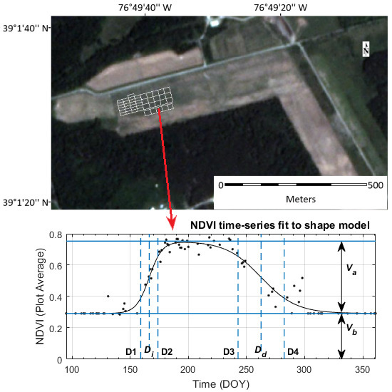
On 9 May 2018, corn (Zea mays L.) was no-till planted in rows spaced 0.76 m apart in a field with crop residues on the soil surface at the United States Department of Agriculture (USDA) Agricultural Research Service (ARS) Henry A. Wallace Beltsville Agricultural Research Center near Beltsville, MD, USA (39.02552 N, 76.82816 W). Best management practices for corn included applying 28 kg N/ha at planting and then additional N several weeks after planting (7 June when the corn plants had 5–7 fully expanded leaves). The additional N rates were 0%, 25%, 50%, 100%, 150%, and 200% of the recommended rate, which was 140 kg N/ha. A randomized block design had two blocks with 9 × 21 m plots and two blocks with 18 × 21 m plots. The additional N rates randomly assigned to plots within each block. Drip irrigation lines were installed on one-half of each plot. Satellite imagery (a PlanetScope image collected on 16 June and processed to surface reflectance) of the site is shown in Figure 1 below.
During the 2018 growing season, in situ measurements were collected approximately once or twice a week. These measurements included leaf chlorophyll content, which was approximated using a Soil Plant Analysis Development (SPAD) meter, and LAI, which was measured using a Li-Cor LAI-2000. The Minolta SPAD-502 meter measures the transmittance of red (650 nm) and infrared (940 nm) radiation through a leaf, and uses these measurements to calculate a SPAD value corresponding to the relative amount of chlorophyll present in that leaf [29]. Although leaf chlorophyll content is typically presented as chlorophyll mass per one-sided leaf unit area, SPAD values are unitless. SPAD measurements have been shown to correlate strongly with lab-extracted leaf chlorophyll measurements for corn and other crops [30]. SPAD values for each plot were reported as an average of 18 measurements: three mid-leaf readings on the topmost fully expanded leaf for six plants near the plot flag. SPAD measurements are used to determine if corn plants are nitrogen deficient, since nitrogen is related to chlorophyll content [31]. LAI is defined as the one-sided green leaf area per unit ground surface area in a vegetation canopy, and is collected using above-and below-canopy radiation measurements. LAI measurements are related to plant biomass and water status; water stress during the vegetative growth stages has been shown to reduce corn plant height and leaf area [32]. Nitrogen stress or water stress during even a small part of the growing season can both reduce corn’s yield [32].
Corn development stages were also measured throughout the growing season. For vegetative stage measurement, one plant on the end of each of the six westernmost plots was flagged above the sixth leaf. When other in situ measurements were collected, the number of fully-expanded leaves on each plant were recorded. Tasseling and silking stages were recorded when tassels and silks became visible on these corn plants. Reproductive stages, including dent and physiological maturity, were estimated based on number of days after silking [33], which has been shown to be more accurate than corn growth models that take into account the daily temperature [34]. More detailed descriptions of the growth stages can be found in Section 3.2.
PlanetScope imagery with 20% or less cloud cover was collected over the Beltsville Airport field between the dates of 1 April and 31 December 2018. This study used the analytic 4-band surface reflectance product provided by Planet [17]. In order to provide this product, Planet processes top-of-atmosphere (TOA) radiance to TOA reflectance using preset coefficients. The surface reflectance is then calculated on a pixel-by-pixel basis using lookup tables (LUTs) generated with the 6SV2.1 radiative transfer code [35]. Surface reflectance images are provided at 3.125 m GSD. Images were downloaded using the now-deprecated Clips API and the Ordersv2 API. A total of 105 images collected over 85 unique days (in a time period spanning 275 days) were downloaded for analysis. Four of the downloaded images were later excluded from the analysis due to quality issues.
Satellite images were processed using ENVI 5.5 (L3Harris Geospatial, Broomfield, CO, USA). After they were converted from GeoTIFF to ENVI format, pixel-based regions of interest (ROIs) (shown in Figure 1) and ROI mask images were created for each plot. They were then loaded into MATLAB R2015b (Mathworks, Natick, MA, USA), where code extracted the Day of Year (DOY), plot-average vegetation index (VI), and the standard deviation of each plot-average VI for every plot in every image. This information was stored in arrays and used for analysis. Note: The PlanetScope imagery was acquired through Planet’s Education and Research Program and may not be shared. All other data are available upon request.
2.2. VI Selection
In order to select the most suitable VI for the temporal resampling portion of the study, two separate analyses were performed. These analyses involved finding the correlations between candidate VIs and ground truth measurements, and calculating and comparing the goodness of fit statistics for candidate VI time-series data fit to a temporal shape model. These analyses are described in the following sections.
2.2.1. VI–Ground Truth Comparison
Candidate VIs were correlated with ground truth information in order to ensure that the VI selected for the shape model fitting analysis was related to crop biophysical parameters. To understand which VIs most correlated with ground truth information, linear regressions were performed between in situ measurements of plot-average SPAD values and Planet-derived plot-average VIs, and between in situ measurements of plot-average LAI values and Planet-derived plot-average VIs. Nine candidate VIs, taken mostly from other papers exploring VI time-series, were considered: Enhanced Vegetation Index (EVI), 2-Band Enhanced Vegetation Index (EVI2), Green Chlorophyll Index (GCI), Green Normalized Difference Vegetation Index (GNDVI), Modified Soil-Adjusted Vegetation Index (MSAVI2), Normalized Difference Vegetation Index (NDVI), Soil-Adjusted Vegetation Index (SAVI), Wide Dynamic Range Vegetation Index (WDRVI, ), and MODIS WDRVI (). MSAVI2 was the only candidate VI that was not drawn from shape model fitting or time-series research; it was considered for this analysis because it is a modification of one of the other indices, SAVI that is intended to reduce increase the dynamic range of the vegetation signal [36]. All of these indices are detailed in Table 1.
There were 11 days of the 2018 growing season in which plot-level SPAD measurements and Planet satellite imagery were both collected: 12 June, 15 June, 18 June, 25 June, 29 June, 3 July, 9 July, 12 July, 17 July, and 24 August. There were five days of the 2018 growing season in which plot-level LAI measurements and Planet satellite imagery were both collected: 15 June, 25 June, 3 July, 11 July (plots 11–26 only), and 16 July (plots 11–64 only). These dates represent crops in both the vegetative and reproductive stages, with a bias towards the first half of the growing season.
Linear regression was performed between all plot-average ground truth measurements for all collection dates and corresponding satellite-derived VIs. Goodness of fit was determined by value.
2.2.2. Shape Model Fitting
The piecewise logistic (also called double logistic or double sigmoid) function was used for shape model fitting. The functional form for the asymmetric double sigmoid function is given in Equation (1), below:
where is the background (i.e., baseline) value, is the amplitude, and represent the dates when the function is increasing or decreasing most rapidly, and p and q relate to the rate of increase or decrease in their respective segments. In addition to and , there are four derivable parameters (, , , and ) that correspond to phenological transition dates. and represent the start and end dates of the period of rapid growth, and and represent the start and end of the period of rapid senescence [25]. These four parameters may be found by finding the local maxima and minima of its second derivative, given in Equation (2) below:
Some of these function parameters may be related to crop-specific phenological stages. In this study, , , , and were tied to field-measured corn development stages (see Table 4 in Section 3.2). Even when not related explicitly to crop phenological stages, these parameters have some uses. They may be used for crop mapping; Zhong et al. found that estimates of the onset () and length () of the growing season could be used to separate field crops from natural vegetation and discriminate between different crop types using MODIS imagery [25]. They may also be used to develop critical parameters for yield prediction; Zhang and Zhang found that the growing season amplitude () and area under the curve () could be related to crop yield [1].
In order to prep the VI time-series for model-fitting, several steps were performed to further clean the data. First, VI values from same-day collects were averaged; this was done so that days in which multiple images were collected would not have extra weight in the fitting process. Next, points from days 198, 228, and 250 were removed for all plots; VI values on these dates were noticeably lower than values on surrounding dates.
Initial fitting tests, as discussed in Section 3.2, were performed with all nine candidate VIs to determine which VI should be used for the temporal sampling analysis. VI time-series data for each plot were cleaned, assigned a new baseline value as described in Section 2.3 below, and fit to the asymmetric double sigmoid function given in Equation (1). Goodness of fit, measured by value and root mean square error (RMSE), was computed for each VI across all plots. NDVI and SAVI (average = 0.922) time-series data had the highest across all plots. NDVI had the lowest RMSE across all plots (average RMSE = 0.047). NDVI was chosen for the shape model fitting. Values of , , , , , and were calculated and averaged across all plots. For each D-value, the ground-measured corn growth stage occurring at the same time was associated with it (e.g., was assumed to mark the beginning of the rapid vegetative growth stage).
2.3. Temporal Sampling and Analysis
Plot-average NDVI time-series were resampled at different temporal revisit rates. Terminology note: In this study, the term “resampling” refers to removing data points from a plot-average NDVI time-series. The resulting points-removed time-series is referred to as the “resampled” time-series. The non-resampled time-series (i.e., the time-series calculated from the complete set of satellite images) are referred to as the “original” time-series. The term “average revisit interval” refers to the average number of days occurring between data points in the NDVI time-series.
In this study, the average revisit interval of the original time-series data was three days. The original time-series data were resampled to create multiple new time series with average revisit intervals ranging from 4 to 24 days, in steps of 1. The method of resampling is as follows. Starting with DOY 95 (the earliest date of PlanetScope imagery collected in this study), sequences of dates were created. These sequences were defined by revisit interval (ranging from every two days to every 25 days, in steps of 1) and offset from the starting date (ranging from 0—i.e., starting at DOY 95—to one day less than the revisit interval). For example, there were two 2-day sequences given by (95, 97, 99, ⋯) and (96, 98, 100, ⋯), three 3-day sequences given by (95, 98, 101, ⋯), (96, 99, 102, ⋯), and (97, 100, 103, ⋯), four 4-day sequences, and so on. Once these sequences were generated, each sequence was iterated through, and the closest available image date for each day in the sequence was selected unless it was a repeat of an already-selected date. The sequences of image dates generated from this selection process were used as the resampled time series data. Average revisit rate was calculated for each of these resampled time series. There were multiple unique time-series for each average revisit interval of the resampled data. All average revisit intervals had eight or more unique time-series, except for the 4-day average revisit interval, which had 4 unique time-series, and the 5-day average revisit interval, which had five unique time-series.
After temporal resampling, the baseline NDVI value ( in Equation (1)) for each time-series was established by finding the average NDVI value of each plot over all post-harvest dates for the resampled time-series. Setting as a constant value is consistent with the approach in another study [45], and performing this procedure after resampling ensured that the effects of resampling were considered in the calculation. Pre-harvest dates were not used to establish because residue from winter rye was still present on the field prior to planting. This crop residue, if included in the calculation, would artificially raise the baseline NDVI. Once was calculated, all NDVI values prior to planting and post-harvest were then replaced with this value.
Curve fitting of the time series data to the asymmetric double sigmoid function was performed using the Curve Fitting Toolbox in Matlab R2015b. Starting assignments for independent variables were: , , , , and . The maximum allowable values of p and q were set to 0.29, which was determined by finding the maximum value of p in initial fitting tests and adding one standard deviation to it. The value of was fixed as the value calculated in the previous step. After fitting, the values of other parameters (, , , and ) were calculated.
Plotwise statistics were calculated across all curve fits for each average revisit interval. For example, there were 17 unique resampled time-series that had an average revisit interval of one image every 16 days, which all gave slightly different phenological transition timing estimates (i.e., , , , , , and values) when curve fitting was performed. From these 17 time-series, the range of values (i.e., maximum–minimum estimate), maximum absolute deviation from the original D value, and average absolute deviation from the original D value were calculated for , , , , , and . This analysis was performed separately for each of the 32 plots. These statistics were then averaged across all plots, plotted as a function of average satellite revisit rate, and fitted to functions. The goal of this analysis was to understand the relationship between increasing satellite revisit interval and variability in estimates of D values, which may be used to estimate corn phenological stages, differentiate corn from other crops, and predict yield.
A graphic representation of the time series analysis and temporal resampling procedure is shown in Figure 3 below.
The temporal resampling procedure and analysis are similar to that of Zhang et al., who considered the sensitivity of vegetation phenology detection to temporal resolution of sampling using MODIS data [6]. However, this study differs from that study in several key ways. First, this study uses VI data derived from imagery, rather than from a simulated time-series. Second, this study considers data at a high spatial resolution (3.125 m GSD), rather than a moderate spatial resolution (250 m GSD). Finally, this study focuses specifically on corn growth and phenology rather than on natural ecosystems.
3. Results
3.1. VI–Ground Truth Comparison
As described in Section 2.2.1, the correlations between candidate VIs and ground truth measurements were used to inform the VI selection for the shape model fitting and temporal resampling analysis. The values of the linear regression between plot-average candidate VIs and plot-average SPAD and LAI measurements are shown in Table 2 below. These candidate VIs were previously defined in Table 1.
As shown in Table 2 above, some indices were more closely correlated with SPAD measurements than others. The best correlations came from NDVI, SAVI, EVI2, and both WDRVI indices.
In the LAI correlation, the three-band EVI (which underperformed in the SPAD) performed similarly to EVI2. Best fits came from EVI, EVI2, NDVI, SAVI, WDRVI ( = 0.1), and WDRVI ( = 0.2), which all performed similarly.
This experiment was used to confirm the VI selection for the shape model fitting experiments. The index selected, based on initial fitting tests (see Section 3.2), NDVI, performed reasonably well in both correlations.
3.2. Shape Model Fitting
VI time-series from all plots were fit to a temporal shape model as described in Section 2.2.2. Goodness of fit results for all indices are presented in Table 3 below. These results, in addition to those of the VI–SPAD and VI–LAI correlations, were also used to inform the selection of VI for the temporal resampling analysis.
Time-series data for all indices generally fit the asymmetric double sigmoid function, although some indices performed slightly better than others in the fitting. NDVI and SAVI had the highest average values across all plots. NDVI and GNDVI had the lowest average RMSE values across all plots. Based on this analysis, as well as the VI–ground truth correlations, NDVI was selected as the index for temporal resampling tests. values for plot-average NDVI time-series data fit to the shape model ranged from 0.788 to 0.963, with an average of 0.922, and RMSE values ranged from 0.039 to 0.061, with an average of 0.045. Only two plots were below an value of 0.85: Plot 53 ( = 0.836, RMSE = 0.055) and Plot 91 ( = 0.788, RMSE = 0.061). These plots also had the two highest RMSE values. Both of these plots were non-irrigated and displayed a significant decrease in NDVI in the middle of the growing season, in response to the drought that occurred in July. Representative plot-average NDVI time-series are shown for four different plots in Figure 4 below.
The average values of , , , , , and across all plots, taken from fitting NDVI time-series data to the asymmetric double sigmoid function, are presented in Table 4 below, along with associated corn growth stages (where they were measured).
In this dataset, some of the function parameters were shown to relate to ground-measured growth stages. Stages V6–7 occurred around . V6 and V7 refer to the emergence of the sixth and seventh leaves of the corn plant, respectively. These stages mark the start of a period of rapid plant growth. Typically nitrogen side-dress (application of additional fertilizer) occurs around V7. Stages V9–10 occurred around . V9 and V10 refer to the emergence of the ninth and tenth leaves of the corn plant, respectively. By stage V10, new leaves will emerge every 2–4 days. The plant’s rate of water and nutrient uptake increases in proportion to its increased rate of growth, and water or nutrient deficiencies at this stage can negatively impact yield. The maximum value of the function, which coincides with the maximum LAI of the corn plant, occurred around VT-R1. VT refers to the stage when the tassel at the top of the corn plant has fully emerged, which marks the end of the vegetative growth stages; R1 refers to the stage when silks become visible outside of the corn husks, which marks the start of the corn reproductive stages. The timing of physiological maturity can be predicted based on the timing of R1. The mid-late Dent stage occurred around . Dent refers to the time when the corn kernels are dying and hardening; stress occurring during this stage can reduce the final weight of the kernels. Physiological maturity occurred around , and corn was ready for harvest around [33]. These findings are consistent with those of another study [24] and demonstrate that parameters from the asymmetric double sigmoid functional fit can be related back to corn phenology for this dataset.
3.3. Temporal Resampling
In Figure 5, Figure 6, Figure 7 and Figure 8, plot-average NDVI time-series data resampled to 8-day, 13-day, 18-day, and 23-day average revisit intervals are shown for the same four plots shown in Figure 4.
Although changes in NDVI can still be witnessed at greater average revisit intervals, the exact fitting parameters and curve shape can change dramatically with fewer sampling points, as shown in the plots above. The following analysis attempts to quantify the effect of increasing revisit interval on changes in and uncertainty of D-value estimates.
Temporal resampling had a minor effect on the spatial variability of D-value estimates. The average values of , , , , , and across all plots did not significantly change with increasing revisit interval, but the standard deviations of , , and estimates across all plots increased from 1–2 days at a 3-day average revisit interval (original time-series, as shown in Table 4) to 3–6 days at a 24-day average revisit interval; this was comparable to the spatial variabilities of , , and estimates, which did not change significantly with increasing revisit interval.
Temporal resampling had a larger effect on temporal variation in D-value estimates. The average absolute deviations of all six D-values from the original D-values at each temporal revisit rate, averaged over all 32 field plots, are shown in Figure 9. All six plots in Figure 9 display a similar behavior of increasing average absolute deviation with increasing average time between images. This result shows that, as the temporal sampling interval increases, estimates of all phenological transition dates vary more and are more dependent on which images are available.
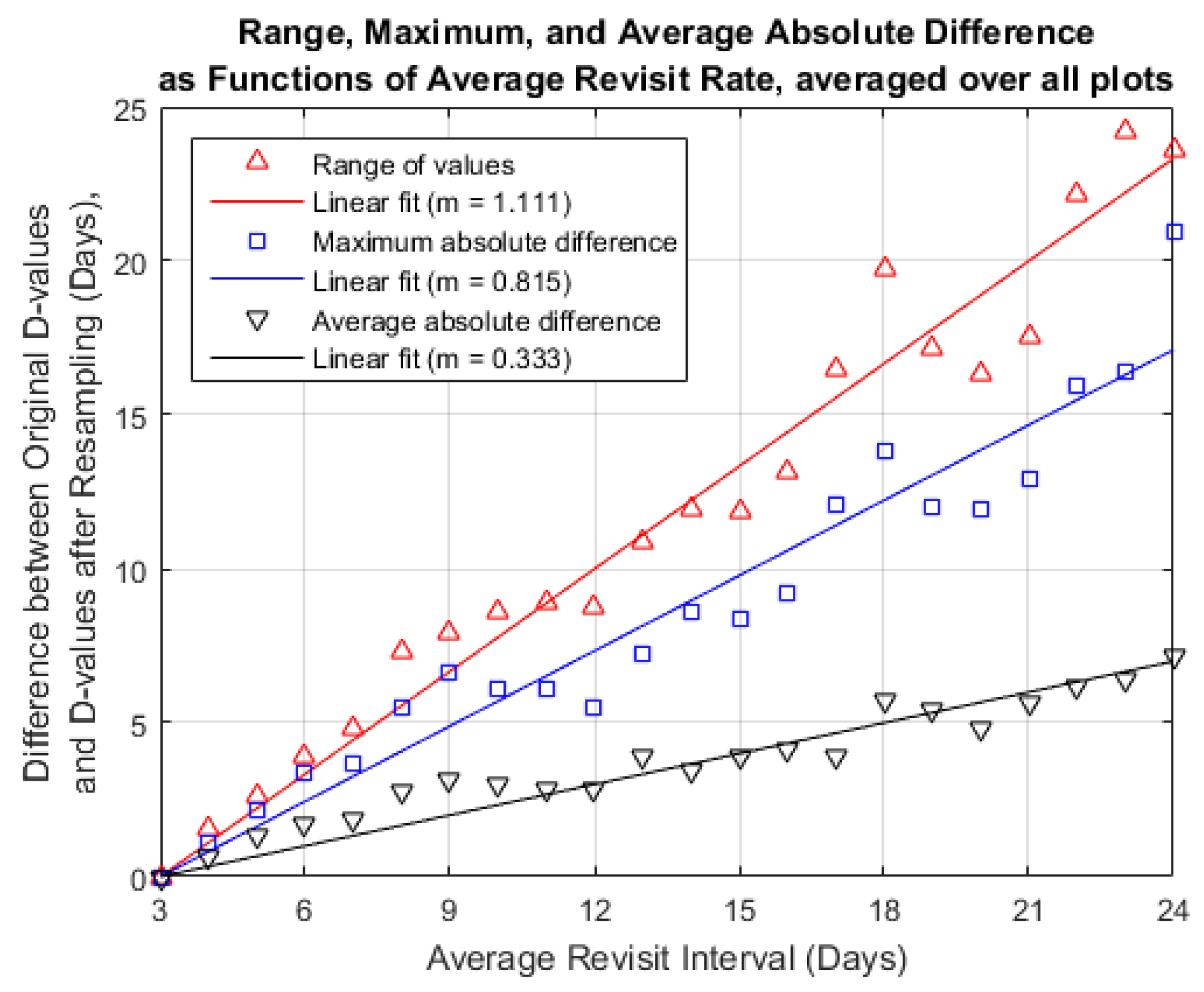
Aside from slight differences in magnitude of changes, all six D-values displayed similar increase in deviation from original values across increasing average revisit interval. Because of this, and for ease of analysis, the performance across all six phenological transition times was averaged for the remaining analysis. Figure 10 shows the range of D-values after temporal resampling, the maximum absolute deviation of post-resampling D-values from original D-values, and the average absolute deviation of post-resampling D-values from original D-values, all as functions of average revisit interval. As described in Section 2.3, these statistics were first calculated separately for each of the 32 plots and each of the six D-values, and were then averaged across all plots and D-values.
As shown in Figure 9 and Figure 10, measured statistics for estimates of phenological transition dates derived from curve-fitting appeared to increase linearly with increase in the average number of days between subsequent images. The statistics considered included: (1) the average absolute deviations of individual D-values from original values, (2) the range of estimated D-values at each revisit interval, averaged over all six D values, (3) the maximum absolute difference between D-values estimated from resampled time-series data and D-values estimated from original time-series data, averaged over all six D values, and (4) the average absolute difference between D-values estimated from resampled time-series data and D-values estimated from original time-series data, averaged over all six D values. The median and mean differences were also calculated. These results are presented in Table 5 below.
The mean and median values of the estimated phenological transition dates shift by less than two days from the original time-series (average 3-day revisit interval) even when the time-series is resampled to an average 24-day revisit interval. However, the maximum, minimum, and average (absolute value) results all show that estimates of phenological transition timing become less precise as sampling interval increases. On average, a 3-day increase in temporal sampling interval (e.g., from one image every three days to one image every six days) will add one day of error onto estimates of D-values which are used as a proxy for corn phenological stages. In a worst-case scenario, that same three-day increase in sampling interval might add closer to two or three days of error onto the estimates, increasing the range of possible values by a little more than three days.
4. Discussion
4.1. VI–Ground Truth Correlation and Initial Shape Model Fitting
The results of the VI–SPAD correlation, VI–LAI correlation, and initial shape model fitting show that the PlanetScope surface reflectance image product may be related to ground-measured phenology, which is consistent with current research [18,19].
As shown in Table 2, the best results of the VIs tested for the SPAD correlation came from those that used only the red and NIR bands: NDVI ( = 0.54), SAVI ( = 0.54), EVI2 ( = 0.54), WDRVI ( = 0.1, = 0.54), and WDRVI ( = 0.2, = 0.53). The indices incorporating blue (EVI) or green bands (GCI, GNDVI) all underperformed in the SPAD correlation compared to these indices. Because the SPAD meter relies on two wavelengths—red (650 nm) and NIR (940 nm)—to estimate relative leaf chlorophyll content [29], it makes sense that the best-performing indices in this correlation all used the same two bands. This relationship held even for two similar indices (EVI and EVI2); the two-band EVI2 showed a stronger correlation with SPAD measurements than the three-band EVI. Since the EVI and EVI2 performed similarly in the LAI correlation, it seems likely that one or more of the images used in the SPAD correlation had calibration issues. A likely source of error is residual cloud or aerosol effects remaining in some of the imagery after atmospheric compensation, which can cause the reflectance in the blue band to appear higher than expected; the creators of EVI2 cite this effect as one of the main sources of large discrepancy between EVI and EVI2 [38]. It is also possible that some of the satellites collecting the imagery over the fields were poorly cross-calibrated with one another. Despite these potential issues with blue band reflectance, the results of this correlation suggest that the red and NIR band spectral reflectances are adequate for characterizing leaf chlorophyll content.
In the LAI correlation, the best results came from EVI ( = 0.78), as well as the indices that performed well in the SPAD correlation: EVI2 ( = 0.76), NDVI ( = 0.77), SAVI ( = 0.77), WDRVI ( = 0.1, = 0.74), and WDRVI ( = 0.2, = 0.75), which all performed similarly. The VI–LAI correlations are generally stronger than the VI–SPAD correlations in this study. This may be because a SPAD meter measures plants at the leaf level, while satellite imagery and LAI measurements both capture properties of the vegetation canopy. Although the best-performing indices correlated reasonably well with LAI measurements, there may have been even more agreement between measured LAI and expected LAI (based on VI correlation) if images and in situ measurements had been collected at the same time. The leaves of the corn plants in this study curled or unfurled in response to water stress, sometimes changing within a relatively short time frame (e.g., hourly). Because in situ LAI was measured either in the early morning or late afternoon (low sun angles are required for the measurements) and Planet overpasses all took place between 11:00 a.m. and 11:30 a.m. local time, it is possible that the in situ measurements might not represent the crop conditions at the time of the image. Disparities between EVI performance in the SPAD and LAI correlations may be caused by improperly-compensated imagery in one or more of the days in which SPAD was collected, which could create artificially high reflectance in the blue band [38]. The results of the SPAD and LAI correlations showed the EVI2, NDVI, SAVI, and both WDRVI indices correlated most strongly with the in situ measurements for this study.
In initial curve-fitting tests, NDVI and SAVI had the highest average values ( = 0.922) across all plots. NDVI and GNDVI had the lowest average RMSE values (NDVI RMSE = 0.045; GNDVI RMSE = 0.046) across all plots. NDVI was selected as the index for the temporal resampling tests.
Ground-measured corn growth stages were related back to D-values estimated from curve-fitting; these included V6-7, which occurred around , V9-10, which occurred around , R5 (Dent), which occurred around , and R6 (Physiological Maturity), which occurred around . There appeared to be more cross-plot variability in the mid-to-late growing season than there was in the early season, with respect to D-value estimates. Whereas the dates of and were relatively constant across all plots, with a standard deviation of only one day, the dates of , , and were much more variable, with standard deviations of 3–5 days. This variability is consistent with the field-measured variability in the growth stages. Variability in plants in the early vegetative stages was observed to be minimal (one leaf difference at most); variability in plants in the late vegetative and reproductive stages was observed to be slightly larger (approximately a week of time difference in observed tasseling dates). This variability is likely due in large part to the differences in irrigation and nitrogen treatment for different plots. Although corn growth rate is heavily tied to temperature, which did not vary spatially across plots, it can also be affected by water and nutrient availability; the presence of environmental stressors can lengthen the time spent in the vegetative (leaf growth) stages and shorten the amount of time spent in the reproductive stages [33]. Differing nitrogen treatments were not applied until a few days before the average occurrence of ; irrigation was not started until early July (3 July: DOY 184, for the small plots, and 6 July: DOY 187, for all plots), which fell after the average occurrence of and before the plot-average NDVI values peaked.
4.2. Temporal Resampling
In the temporal resampling analysis, the average absolute deviations of individual D-values from their original values were considered separately. Although average absolute deviation appeared to increase for all D-values with increasing revisit interval, had the greatest amount of deviation in estimates even at higher frequency sampling. Referring back to Figure 2, which shows an NDVI time-series derived from one of the 32 plots, it is clear that there is significant fluctuation between the image-to-image measurements of NDVI around . The fluctuations in late-season NDVI exhibited by this plot are representative of fluctuations exhibited by all plots in the study. For plot 74 in particular (the plot pictured in Figure 2), the NDVI values between DOY 159 and DOY 298 ranged between 0.29 and 0.52. Some amount of fluctuation may be attributable to errors in atmospheric compensation, cross-satellite calibration, or differences in illumination conditions day-to-day [22], but the fluctuations around in particular may be caused by natural vegetation (grasses, weeds, etc.) growing around and underneath the corn canopy. When corn plants reach maturity, many of their leaves are dry and yellow [33], meaning that they do not contribute strongly to NDVI or other vegetation indices. Differences in wind and other daily conditions may have caused this natural vegetation underneath the canopy to be more or less visible to the satellite sensors on some collection dates. It is also worth noting that there was a 20-day gap in the imagery during the senescence period, between images collected on 6 September (DOY 249) and 26 September (DOY 269). While this gap in the data may not have affected specifically, it may have made D-values occurring near or within this gap (, , and ) more difficult to fit accurately.
When the performance across all six D-values was averaged, all measured statistics for estimates of phenological transition dates derived from curve-fitting appeared to increase linearly with increase in the average number of days between subsequent images. These statistics included: (1) the range of estimated D-values at each revisit interval, averaged over all six D values, (2) the maximum absolute difference between D-values estimated from resampled time-series data and D-values estimated from original time-series data, averaged over all six D values, and (3) the average absolute difference between D-values estimated from resampled time-series data and D-values estimated from original time-series data, averaged over all six D values. On average, a 3-day increase in temporal sampling interval (e.g., from one image every three days to one image every six days) was found to add one day of error onto estimates of D-values which are used as a proxy for corn phenological stages. In a worst-case scenario, that same 3-day increase in sampling interval might add closer to two or three days of error onto the estimates, increasing the range of possible values by a little more than three days.
Changes in the estimated timing of , , , and will affect the image-based estimation of the associated corn phenological stages described in Table 4. If significant enough, these uncertainties could lead to errors in crop management (e.g., applying additional nitrogen fertilizer too early or too late in the growing season). Additionally, errors in D-value estimation may lead to error in remote sensing tasks that rely on these D-values and associated VI values in order to make predictions, as described in Section 2.2.2.
Both the apparent linear increase in error with increasing sampling interval and the approximate rate of increase are consistent with the result obtained from the modeled (i.e., ideal, non-noise-added) data from the study of Zhang et al. [6], which performed a similar analysis using MODIS-derived EVI time-series data. This study contributes uniquely to previous literature, however, in that it uses very high spatial resolution (pixel size < 10 m) satellite imagery for this temporal sampling analysis. Because image heterogeneity, which is affected by pixel size, is an important consideration in agricultural monitoring [9], and because recent agricultural monitoring efforts have been shifting towards the use of higher spatial resolution data [14,16,23], it is important to understand how these effects play out in high spatial resolution systems.
This work builds on previous studies defining temporal sampling requirements for cloud-free imaging [7] and for “reasonably clear” (70–95% cloud-free) imaging of agriculture [8] by considering the specific effect of temporal revisit intervals on corn phenology monitoring via shape model fitting. The parameters obtained from shape model fitting may be used, as they were in this study, to estimate corn phenological stages and approximate phenological transition timing. In other studies, these same parameters have been used for agricultural remote sensing tasks including crop mapping [25] and yield prediction [1].
4.3. Limitations and Sources of Error
There are a few limitations to this study. First, it is small, representing only one crop (corn) over a small area, meaning that the results may not generalize to all crops, locations, and growing conditions. Image availability was also limited to the images the PlanetScope constellation was able to collect, meaning that some portions of the time-series had gaps due to cloud cover and other collection issues even before data points were removed.
Second, initial values of curve fitting parameters were observed to have a small effect on final fitting results. While the authors selected these values based on initial curve-fitting tests and kept them consistent across all curve fits, it is possible that changes in these parameters could have minor impacts on goodness of fit or transition timing estimates for some of the plots.
Finally, the PlanetScope satellites provide imagery that is of low radiometric quality compared to imagery from satellites like Landsat 8 or Sentinel 2 [22]. Large day-to-day changes in average NDVI can be observed in Figure 2. Some of these day-to-day changes may be attributable to ground-observable differences in the corn, such as decreases in visible leaf area when leaves curl in hot weather, or slight differences in time of collection, which generally occurred at the same time of day within a thirty-minute window. However, many of these changes in the imagery are likely not attributable to actual changes on the ground. Some possible sources of noise include poor cross-sensor calibration and limited atmospheric compensation. The PlanetScope surface reflectance product used in this study is limited in several ways: it does not correct for haze or thin cirrus clouds, it uses a single global model for aerosols, and it does not account for bidirectional reflectance distribution function (BRDF) effects, stray light, or adjacency effects [46]. In the VI–SPAD correlation, it was observed that EVI and EVI2 differed significantly, an effect that is most likely attributed to undetected atmospheric water vapor or aerosols affecting the retrieved reflectance spectra. A less noisy time series might achieve similar estimation accuracy with fewer data points.
5. Conclusions
In this study, we have quantified the impact of temporal sampling frequency on our ability to accurately estimate corn phenological transition timing from high-resolution satellite imagery. Using high-frequency PlanetScope imagery of a corn field in Maryland, we generated plot-average NDVI time-series data, fit the data to an asymmetric double sigmoid function, and used curve-fitting parameters to derive corn phenological stages. After initial fitting, images were removed from the time-series and fitting was performed on the sampled time-series to see how image frequency affected the results. Both average and maximum errors in estimates were shown to increase linearly with increase in average temporal spacing between images. On average, a 3-day increase in temporal sampling interval was found to add one day of error onto phenological transition timing estimates; maximally, a 3-day increase in temporal sampling interval was found to add closer to two or three days of error onto the same estimates. To the best of our knowledge, this is the first study to derive a quantitative relationship between satellite revisit interval and accuracy of shape model fitting parameter estimation for very high resolution (<10 m GSD) imagery, which may prove important for near-daily observation of farms that cannot be resolved by coarser sensors like MODIS.
Future work is planned to address the primary limitations of this study, which are its small size and its reliance on the PlanetScope satellites. In situ measurements and imagery are being re-collected over the same corn fields during the 2019 growing season in order to add to the robustness of these results. Additionally, PlanetScope imagery from the 2019 growing season will be compared with imagery from several other satellite systems of higher radiometric quality in order to investigate the trade-offs of spectral, spatial, and temporal resolutions on ability to monitor crop growth. Although the authors of this study do not currently plan to look at other crops, other researchers may easily apply these methods to other crops, locations, and sensors in order to gain an understanding of how these results vary for different scenarios. Future work will also focus on relating shape model fitting parameters and phenological transition timing estimates to yield prediction for this dataset.
Despite the limited scope of this study, these results show that CubeSats can be used for corn monitoring and phenological transition timing estimates, and that less frequent observations lead to linearly increasing error in these estimates. This study provides a guideline for determining the necessary observation frequency for agricultural monitoring via shape model fitting, depending on the need for precision in the specific monitoring application, and provides a novel contribution to ongoing research into temporal and spatial image requirements for agricultural monitoring needs.
References
Author Contributions
Conceptualization, E.M.; Formal analysis, E.M.; Investigation, E.M., C.D., and A.R.; Resources, C.D. and A.R.; Supervision, J.K.; Writing—original draft, E.M.; Writing—review and editing, E.M., J.K., C.D., and A.R.
Funding
This work has been supported in part by the National Aeronautics and Space Administration under Grant No. NNX14AP40G.
Acknowledgments
The authors would like to thank Planet Labs, Inc. (San Francisco, CA, USA) for providing us with the imagery used in this study.
Conflicts of Interest
The authors declare no conflict of interest.
References
- Zhang, X.; Zhang, Q. Monitoring interannual variation in global crop yield using long-term AVHRR and MODIS observations. ISPRS J. Photogramm. Remote. Sens. 2016, 114, 191–205. [Google Scholar] [CrossRef]
- Sakamoto, T. Refined shape model fitting methods for detecting various types of phenological information on major U.S. crops. ISPRS J. Photogramm. Remote. Sens. 2018, 138, 176–192. [Google Scholar] [CrossRef]
- Zhang, X.; Wang, J.; Gao, F.; Liu, Y.; Schaaf, C.; Friedl, M.; Yu, Y.; Jayavelu, S.; Gray, J.; Liu, L.; et al. Exploration of scaling effects on coarse resolution land surface phenology. Remote Sens. Environ. 2017, 190, 318–330. [Google Scholar] [CrossRef] [Green Version]
- González-Sanpedro, M.; Le Toan, T.; Moreno, J.; Kergoat, L.; Rubio, E. Seasonal variations of leaf area index of agricultural fields retrieved from Landsat data. Remote Sens. Environ. 2008, 112, 810–824. [Google Scholar] [CrossRef] [Green Version]
- Jönsson, P.; Cai, Z.; Melaas, E.; Friedl, M.; Eklundh, L. A Method for Robust Estimation of Vegetation Seasonality from Landsat and Sentinel-2 Time Series Data. Remote Sens. 2018, 10, 635. [Google Scholar] [CrossRef]
- Zhang, X.; Friedl, M.A.; Schaaf, C.B. Sensitivity of vegetation phenology detection to the temporal resolution of satellite data. Int. J. Remote. Sens. 2009, 30, 2061–2074. [Google Scholar] [CrossRef]
- Goward, S.N.; Loboda, T.V.; Williams, D.L.; Huang, C. Landsat Orbital Repeat Frequency and Cloud Contamination: A Case Study for Eastern United States. Photogramm. Eng. Remote Sens. 2019, 85, 109–118. [Google Scholar] [CrossRef]
- Whitcraft, A.; Becker-Reshef, I.; Justice, C. A Framework for Defining Spatially Explicit Earth Observation Requirements for a Global Agricultural Monitoring Initiative (GEOGLAM). Remote Sens. 2015, 7, 1461–1481. [Google Scholar] [CrossRef] [Green Version]
- Löw, F.; Duveiller, G. Defining the Spatial Resolution Requirements for Crop Identification Using Optical Remote Sensing. Remote Sens. 2014, 6, 9034–9063. [Google Scholar] [CrossRef] [Green Version]
- Gao, F.; Masek, J.; Schwaller, M.; Hall, F. On the blending of the Landsat and MODIS surface reflectance: predicting daily Landsat surface reflectance. IEEE Trans. Geosci. Remote Sens. 2006, 44, 2207–2218. [Google Scholar] [CrossRef]
- Meng, J.; Du, X.; Wu, B. Generation of high spatial and temporal resolution NDVI and its application in crop biomass estimation. Int. J. Digit. Earth 2013, 6, 203–218. [Google Scholar] [CrossRef]
- Walker, J.; de Beurs, K.; Wynne, R.; Gao, F. Evaluation of Landsat and MODIS data fusion products for analysis of dryland forest phenology. Remote Sens. Environ. 2012, 117, 381–393. [Google Scholar] [CrossRef]
- Li, J.; Roy, D. A Global Analysis of Sentinel-2A, Sentinel-2B and Landsat-8 Data Revisit Intervals and Implications for Terrestrial Monitoring. Remote Sens. 2017, 9, 902. [Google Scholar] [CrossRef]
- Claverie, M.; Ju, J.; Masek, J.G.; Dungan, J.L.; Vermote, E.F.; Roger, J.C.; Skakun, S.V.; Justice, C. The Harmonized Landsat and Sentinel-2 surface reflectance data set. Remote Sens. Environ. 2018, 219, 145–161. [Google Scholar] [CrossRef]
- Liu, Y.; Hill, M.J.; Zhang, X.; Wang, Z.; Richardson, A.D.; Hufkens, K.; Filippa, G.; Baldocchi, D.D.; Ma, S.; Verfaillie, J.; et al. Using data from Landsat, MODIS, VIIRS and PhenoCams to monitor the phenology of California oak/grass savanna and open grassland across spatial scales. Agric. For. Meteorol. 2017, 237-238, 311–325. [Google Scholar] [CrossRef]
- Wu, Z.; Snyder, G.; Vadnais, C.; Arora, R.; Babcock, M.; Stensaas, G.; Doucette, P.; Newman, T. User needs for future Landsat missions. Remote Sens. Environ. 2019, 231, 111214. [Google Scholar] [CrossRef]
- Planet Team. Planet Application Program Interface: In Space for Life on Earth; Planet Team: San Francisco, CA, USA, 2017; Available online: https://api.planet.com (accessed on 1 May 2019).
- Sadeh, Y.; Zhu, X.; Chenu, K.; Dunkerley, D. Sowing date detection at the field scale using CubeSats remote sensing. Comput. Electron. Agric. 2019, 157, 568–580. [Google Scholar] [CrossRef]
- Helman, D.; Bahat, I.; Netzer, Y.; Ben-Gal, A.; Alchanatis, V.; Peeters, A.; Cohen, Y. Using Time Series of High-Resolution Planet Satellite Images to Monitor Grapevine Stem Water Potential in Commercial Vineyards. Remote Sens. 2018, 10, 1615. [Google Scholar] [CrossRef]
- Burke, M.; Lobell, D.B. Satellite-based assessment of yield variation and its determinants in smallholder African systems. Proc. Natl. Acad. Sci. USA 2017, 114, 2189–2194. [Google Scholar] [CrossRef] [Green Version]
- Kross, A.; McNairn, H.; Lapen, D.; Sunohara, M.; Champagne, C. Assessment of RapidEye vegetation indices for estimation of leaf area index and biomass in corn and soybean crops. Int. J. Appl. Earth Obs. Geoinf. 2015, 34, 235–248. [Google Scholar] [CrossRef] [Green Version]
- Houborg, R.; McCabe, M.F. A Cubesat enabled Spatio-Temporal Enhancement Method (CESTEM) utilizing Planet, Landsat and MODIS data. Remote Sens. Environ. 2018, 209, 211–226. [Google Scholar] [CrossRef]
- Houborg, R.; McCabe, M. Daily Retrieval of NDVI and LAI at 3 m Resolution via the Fusion of CubeSat, Landsat, and MODIS Data. Remote Sens. 2018, 10, 890. [Google Scholar] [CrossRef]
- Gao, F.; Anderson, M.C.; Zhang, X.; Yang, Z.; Alfieri, J.G.; Kustas, W.P.; Mueller, R.; Johnson, D.M.; Prueger, J.H. Toward mapping crop progress at field scales through fusion of Landsat and MODIS imagery. Remote Sens. Environ. 2017, 188, 9–25. [Google Scholar] [CrossRef] [Green Version]
- Zhong, L.; Hu, L.; Yu, L.; Gong, P.; Biging, G.S. Automated mapping of soybean and corn using phenology. ISPRS J. Photogramm. Remote Sens. 2016, 119, 151–164. [Google Scholar] [CrossRef] [Green Version]
- Zhang, X.; Friedl, M.A.; Schaaf, C.B.; Strahler, A.H.; Hodges, J.C.; Gao, F.; Reed, B.C.; Huete, A. Monitoring vegetation phenology using MODIS. Remote Sens. Environ. 2003, 84, 471–475. [Google Scholar] [CrossRef]
- Hong, S.Y.; Sudduth, K.A.; Kitchen, N.R.; Fraisse, C.W.; Palm, H.L.; Wiebold, W.J. Comparison of Remote Sensing and Crop Growth Models for Estimating Within-Field LAI Variability. Korean J. Remote Sens. 2004, 20, 14. [Google Scholar]
- White, K.; Pontius, J.; Schaberg, P. Remote sensing of spring phenology in northeastern forests: A comparison of methods, field metrics and sources of uncertainty. Remote Sens. Environ. 2014, 148, 97–107. [Google Scholar] [CrossRef]
- Uddling, J.; Gelang-Alfredsson, J.; Piikki, K.; Pleijel, H. Evaluating the relationship between leaf chlorophyll concentration and SPAD-502 chlorophyll meter readings. Photosynth. Res. 2007, 91, 37–46. [Google Scholar] [CrossRef]
- Xiong, D.; Chen, J.; Yu, T.; Gao, W.; Ling, X.; Li, Y.; Peng, S.; Huang, J. SPAD-based leaf nitrogen estimation is impacted by environmental factors and crop leaf characteristics. Sci. Rep. 2015, 5. [Google Scholar] [CrossRef]
- Bullock, D.G.; Anderson, D.S. Evaluation of the Minolta SPAD-502 chlorophyll meter for nitrogen management in corn. J. Plant Nutr. 1998, 21, 741–755. [Google Scholar] [CrossRef]
- Çakir, R. Effect of water stress at different development stages on vegetative and reproductive growth of corn. Field Crop. Res. 2004, 89, 1–16. [Google Scholar] [CrossRef]
- Ritchie, S.; Hanway, J.; Benson, G. How a Corn Plant Develops; Special Report No. 48; Iowa State University, Cooperative Extension Service: Ames, IA, USA, 2005. [Google Scholar]
- Daughtry, C.S.T.; Cochran, J.C.; Hollinger, S.E. Estimating Silking and Maturity Dates of Corn for Large Areas1. Agron. J. 1984, 76, 415. [Google Scholar] [CrossRef]
- Marta, S. Planet Imagery Product Specifications; Planet Labs: San Francisco, CA, USA, 2018; p. 91. [Google Scholar]
- Qi, J.; Chehbouni, A.; Huete, A.; Kerr, Y.; Sorooshian, S. A modified soil adjusted vegetation index. Remote Sens. Environ. 1994, 48, 119–126. [Google Scholar] [CrossRef]
- Huete, A.; Didan, K.; Miura, T.; Rodriguez, E.; Gao, X.; Ferreira, L. Overview of the radiometric and biophysical performance of the MODIS vegetation indices. Remote Sens. Environ. 2002, 83, 195–213. [Google Scholar] [CrossRef]
- Jiang, Z.; Huete, A.; Didan, K.; Miura, T. Development of a two-band enhanced vegetation index without a blue band. Remote Sens. Environ. 2008, 112, 3833–3845. [Google Scholar] [CrossRef]
- Gitelson, A.A.; Gritz, Y.; Merzlyak, M.N. Relationships between leaf chlorophyll content and spectral reflectance and algorithms for non-destructive chlorophyll assessment in higher plant leaves. J. Plant Physiol. 2003, 160, 271–282. [Google Scholar] [CrossRef]
- Rouse, J.; Haas, R.; Schell, J.; Deering, D. Monitoring Vegetation Systems in the Great Plains with ERTS; NASA: Washington, DC, USA, 1973.
- Huete, A. A soil-adjusted vegetation index (SAVI). Remote Sens. Environ. 1988, 25, 295–309. [Google Scholar] [CrossRef]
- Gitelson, A.A. Wide Dynamic Range Vegetation Index for Remote Quantification of Biophysical Characteristics of Vegetation. J. Plant Physiol. 2004, 161, 165–173. [Google Scholar] [CrossRef] [Green Version]
- Sakamoto, T.; Gitelson, A.A.; Arkebauer, T.J. MODIS-based corn grain yield estimation model incorporating crop phenology information. Remote. Sens. Environ. 2013, 131, 215–231. [Google Scholar] [CrossRef]
- Henebry, G.M.; Viña, A.; Gitelson, A.A. The Wide Dynamic Range Vegetation Index and its Potential Utility for Gap Analysis. Gap Anal. Bull. 2004, 12, 50–56. [Google Scholar]
- Zhang, X. Reconstruction of a complete global time series of daily vegetation index trajectory from long-term AVHRR data. Remote Sens. Environ. 2015, 156, 457–472. [Google Scholar] [CrossRef]
- Collison, A.; Wilson, N. Planet Surface Reflectance Product; Planet Labs: San Francisco, CA, USA, 2018. [Google Scholar]
Figure 1.
(a) View of the field and plot locations. (b) contrast-enhanced, closer view of the plots. Both images show RGB surface reflectance, derived from imagery collected by a PlanetScope satellite on 16 June 2018. Each plot is represented as a white box. The smaller plots are roughly 9 by 21 m, and the larger plots are roughly 18 by 21 m. The plots in the third and fourth columns from the left (the two columns of small plots closest to the larger plots) were excluded from analysis due to treatment errors.

Figure 2.
Asymmetric double sigmoid function fit to NDVI time-series for one of the corn subplots (Plot 74), with function parameters labeled. This figure shows original (non-resampled) time-series data, which had an average revisit interval of three days.
Figure 2.
Asymmetric double sigmoid function fit to NDVI time-series for one of the corn subplots (Plot 74), with function parameters labeled. This figure shows original (non-resampled) time-series data, which had an average revisit interval of three days.
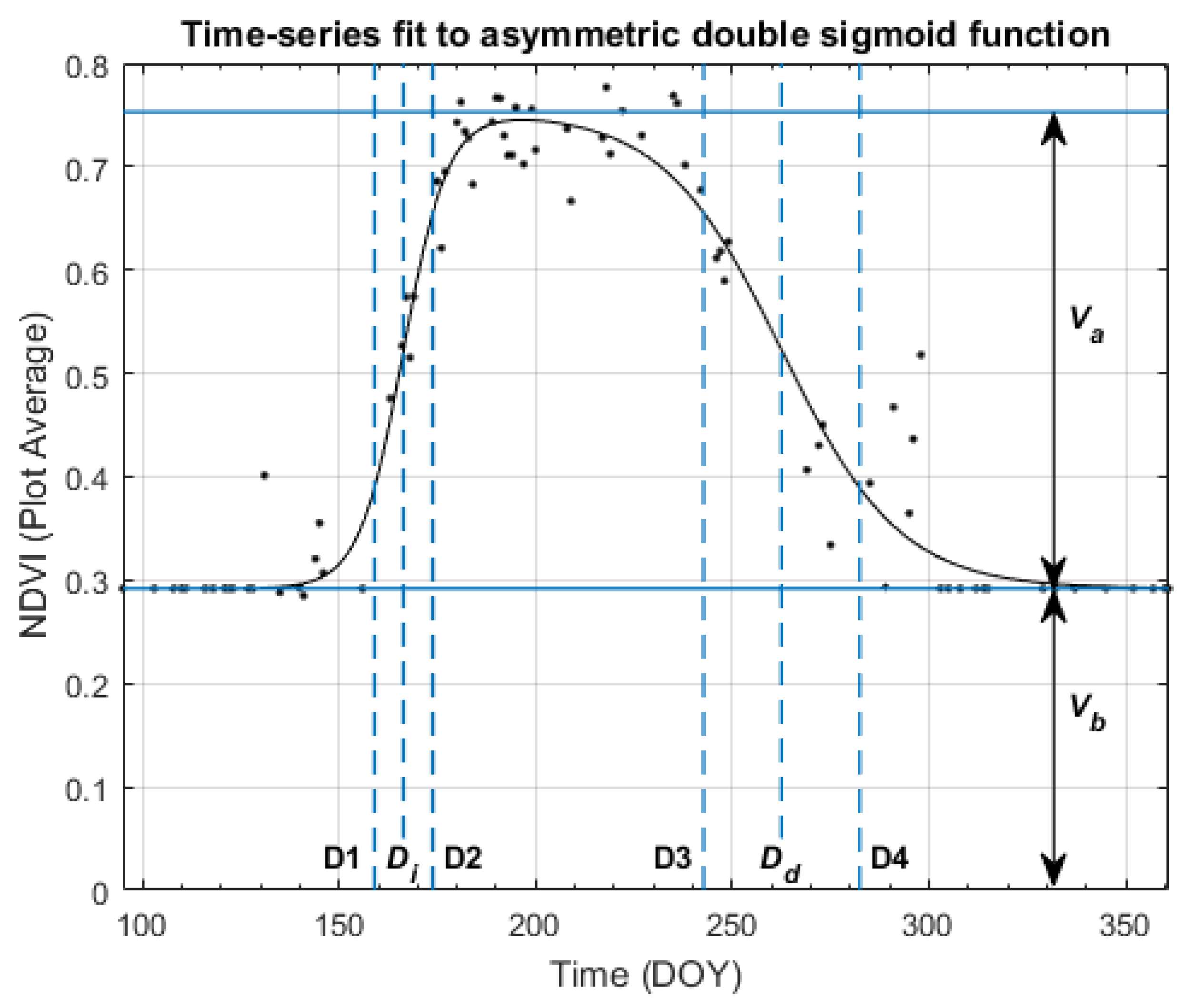
Figure 3.
Visual representation of the temporal resampling procedure and analysis. All steps are described in more detail in the Methods section. Note: This analysis was performed separately for each of the 32 plots shown in Figure 1. After the end results (range, maximum absolute deviation, and average absolute deviation as a function of revisit interval) were obtained, they were averaged across all 32 plots.

Figure 4.
Four different plot-average NDVI time-series fit to the asymmetric double sigmoid function. Plot 63 was non-irrigated and treated with 200% N, Plot 94 was non-irrigated and treated with 0% N, Plot 82 was irrigated and treated with 50% N, and Plot 24 was irrigated and treated with 75% N.
Figure 4.
Four different plot-average NDVI time-series fit to the asymmetric double sigmoid function. Plot 63 was non-irrigated and treated with 200% N, Plot 94 was non-irrigated and treated with 0% N, Plot 82 was irrigated and treated with 50% N, and Plot 24 was irrigated and treated with 75% N.
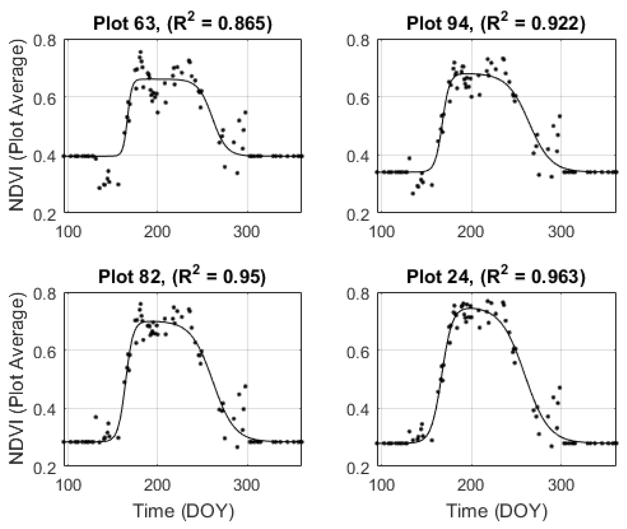
Figure 5.
Four different plot-average NDVI time-series resampled to an 8-day average revisit interval and fit to the asymmetric double sigmoid function.
Figure 5.
Four different plot-average NDVI time-series resampled to an 8-day average revisit interval and fit to the asymmetric double sigmoid function.

Figure 6.
Four different plot-average NDVI time-series resampled to a 13-day average revisit interval and fit to the asymmetric double sigmoid function.
Figure 6.
Four different plot-average NDVI time-series resampled to a 13-day average revisit interval and fit to the asymmetric double sigmoid function.

Figure 7.
Four different plot-average NDVI time-series resampled to an 18-day average revisit interval and fit to the asymmetric double sigmoid function.
Figure 7.
Four different plot-average NDVI time-series resampled to an 18-day average revisit interval and fit to the asymmetric double sigmoid function.
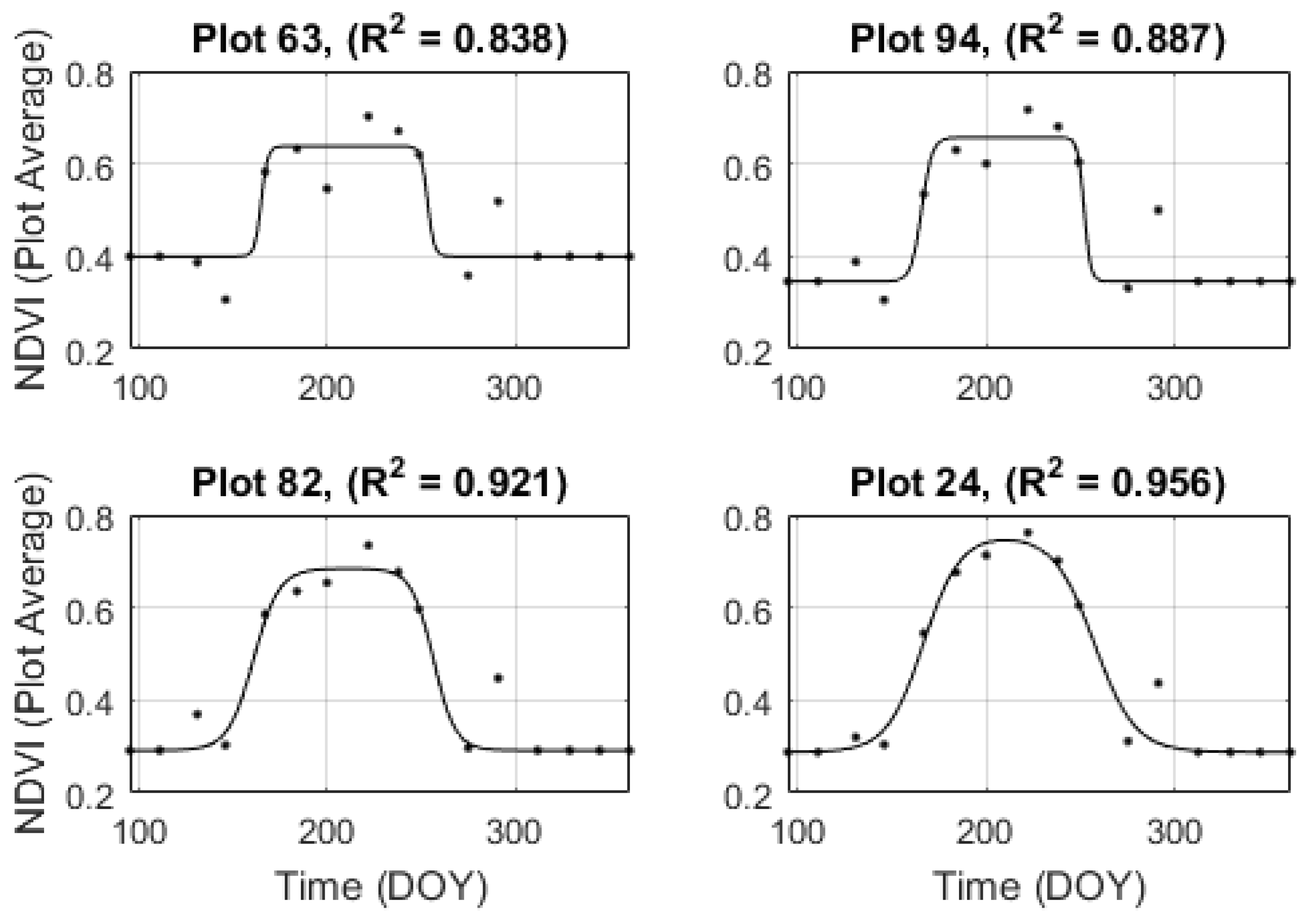
Figure 8.
Four different plot-average NDVI time-series resampled to a 23-day average revisit interval and fit to the asymmetric double sigmoid function.
Figure 8.
Four different plot-average NDVI time-series resampled to a 23-day average revisit interval and fit to the asymmetric double sigmoid function.

Figure 9.
Average absolute deviations of , , , , , and from the original D-values, shown as a function of average temporal revisit rate. Each data point represents the deviation of the calculated D-value across all resampled time-series at that particular image frequency. These statistics were collected separately for each individual plot and were then averaged for analysis; the data points presented above represent the average of statistics across all 32 plots.
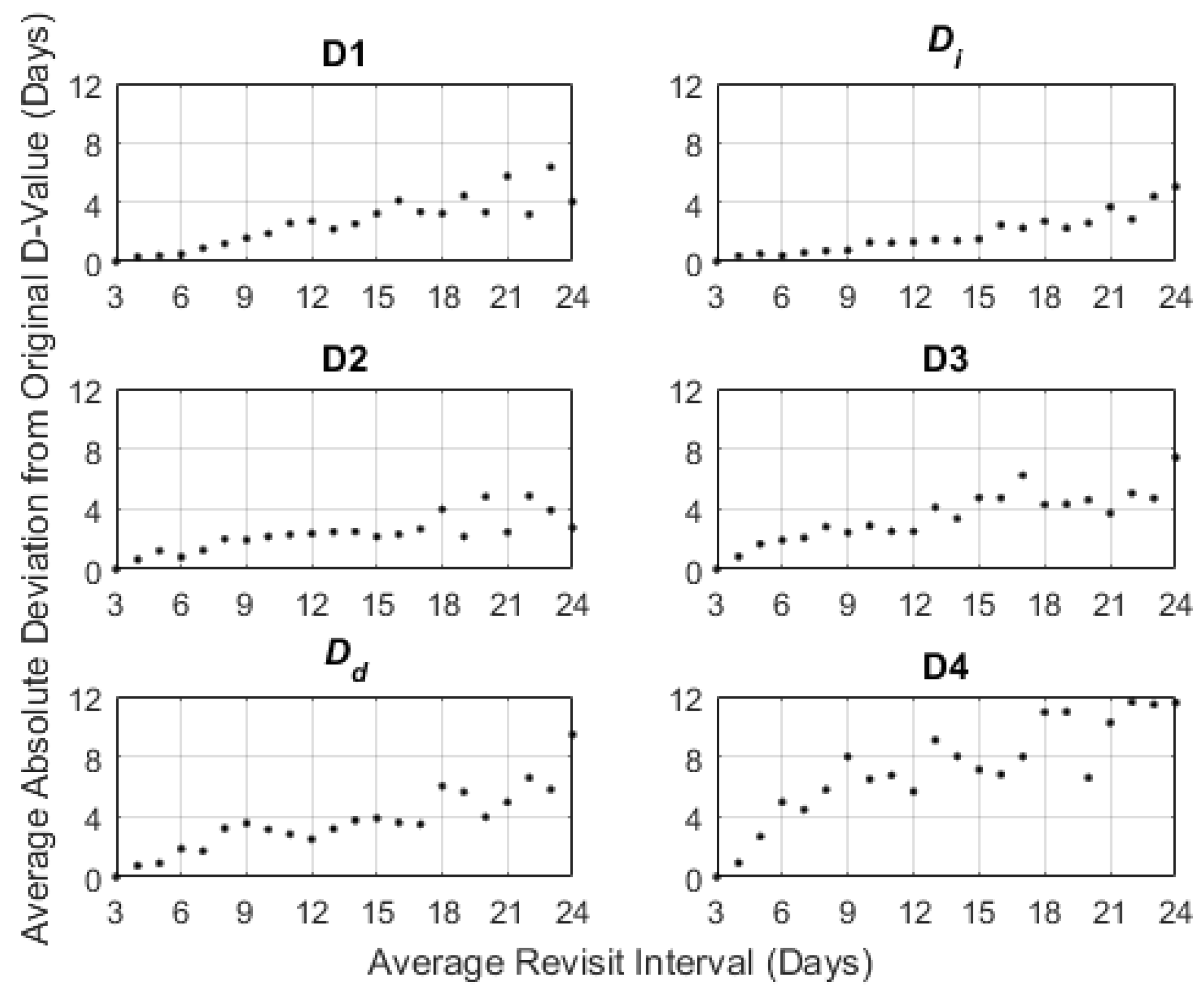
Figure 10.
Range of D-values after temporal resampling, maximum absolute deviation of post-resampling D-values from original D-value, and average absolute deviation of post-resampling D-values from original D-value, shown as functions of average revisit interval. These statistics were collected separately for each individual D-value and each individual plot and were then averaged for analysis; the data points presented above represent the average of statistics across all six D-values and all 32 plots.

Table 1.
Candidate vegetation indices, their equations, references to the papers in which they were proposed, and references to papers that use them for agricultural monitoring or related purposes. In the equations, refers to reflectance in the blue wavelength band, refers to reflectance in the green wavelength band, refers to reflectance in the red wavelength band, and refers to reflectance in the NIR wavelength band. Non-abbreviated forms of the indices’ names can be found in the text immediately preceding the table and in the references to the indices’ originating research.
| Index | Equation | Originating Research | Citing Research |
|---|---|---|---|
| EVI | [37] | [25,26] | |
| EVI2 | [38] | [1] | |
| GCI | [39] | [20] | |
| GNDVI | [39] | [19] | |
| MSAVI2 | [36] | ||
| NDVI | [40] | [24] | |
| SAVI | [41] | [27] | |
| WDRVI, = 0.1 | [42] | [43] | |
| WDRVI, = 0.2 | [42,44] | [43] |
Table 2.
Candidate vegetation indices, the relevant image bands, the value of their linear correlation with Soil Plant Analysis Development (SPAD) measurements, and the value of their linear correlation with leaf area index (LAI) measurements.
Table 2.
Candidate vegetation indices, the relevant image bands, the value of their linear correlation with Soil Plant Analysis Development (SPAD) measurements, and the value of their linear correlation with leaf area index (LAI) measurements.
| Vegetation Index | Bands Used | SPAD Value | LAI Value |
|---|---|---|---|
| EVI | Blue, Red, NIR | 0.37 | 0.78 |
| EVI2 | Red, NIR | 0.54 | 0.76 |
| GCI | Green, NIR | 0.45 | 0.40 |
| GNDVI | Green, NIR | 0.46 | 0.46 |
| MSAVI2 | Red, NIR | 0.34 | 0.50 |
| NDVI | Red, NIR | 0.54 | 0.77 |
| SAVI | Red, NIR | 0.54 | 0.77 |
| WDRVI, = 0.1 | Red, NIR | 0.54 | 0.74 |
| WDRVI, = 0.2 | Red, NIR | 0.53 | 0.75 |
Table 3.
Candidate vegetation indices, the value of their fit to the asymmetric double sigmoid function, averaged across all plots, and the root mean square error (RMSE) value of their fit to the asymmetric double sigmoid function, averaged across all plots. Unlike most of the indices, Green Chlorophyll Index (GCI) and Modified Soil-Adjusted Vegetation Index 2 (MSAVI2) are not scaled between −1 and 1, so their RMSE values cannot be directly compared with those of the other indices.
| Vegetation Index | Value | RMSE |
|---|---|---|
| EVI | 0.765 | 0.313 |
| EVI2 | 0.917 | 0.108 |
| GCI | 0.836 | 0.513 |
| GNDVI | 0.869 | 0.046 |
| MSAVI2 | 0.502 | 869.378 |
| NDVI | 0.922 | 0.045 |
| SAVI | 0.922 | 0.067 |
| WDRVI, = 0.1 | 0.898 | 0.052 |
| WDRVI, = 0.2 | 0.908 | 0.062 |
Table 4.
Average values of , , , , , and across all plots, with standard deviations included, related to field-measured corn growth stages when applicable. Descriptions of corn growth stages are taken from [33]. Although it was not considered in the resampling analysis, the location of the function maximum was shown to occur at the same time as the corn plant tasseling.
| Function Parameter | DOY | Associated Development Stage | Description |
|---|---|---|---|
| 161 ± 1 | V6–7 | Beginning of rapid vegetative growth. | |
| 166 ± 1 | V9–10 | Rapid growth, with a new fully expanded leaf every 2–4 days. | |
| 171 ± 2 | Rapid stalk elongation | Corn plants are growing taller. | |
| Maximum | 193 ± 4 | VT-R1 | Tassel fully emerged and all leaves fully expanded. End of vegetative growth—reproductive stages start when any silks become visible. |
| 248 ± 5 | R5—Mid-late Dent | Starch in kernels is drying and hardening. | |
| 264 ± 3 | R6—Physiological Maturity | Maximum grain dry matter accumulation, with a grain moisture content of 30–35%. | |
| 280 ± 4 | Harvest Maturity | Harvest occurs after grain is dried to <20% moisture; grain is safely stored at <15% moisture. |
Table 5.
Statistics used for assessing the impact of average temporal revisit rate on phenological transition timing estimation. The slope of linear fit refers to the slope of the named statistic vs. the average temporal revisit rate.
Table 5.
Statistics used for assessing the impact of average temporal revisit rate on phenological transition timing estimation. The slope of linear fit refers to the slope of the named statistic vs. the average temporal revisit rate.
| Metric (Days) | Slope of Linear Fit | |
|---|---|---|
| Median difference | −0.049 | −0.12 |
| Mean difference | −0.029 | −0.06 |
| Average absolute difference | 0.333 | 0.91 |
| Maximum absolute difference | 0.864 | 0.93 |
| Difference range (Maximum − Minimum) | 1.111 | 0.96 |
© 2019 by the authors. Licensee MDPI, Basel, Switzerland. This article is an open access article distributed under the terms and conditions of the Creative Commons Attribution (CC BY) license (http://creativecommons.org/licenses/by/4.0/).
Share and Cite
MDPI and ACS Style
Myers, E.; Kerekes, J.; Daughtry, C.; Russ, A. Assessing the Impact of Satellite Revisit Rate on Estimation of Corn Phenological Transition Timing through Shape Model Fitting. Remote Sens. 2019, 11, 2558. https://doi.org/10.3390/rs11212558
AMA Style
Myers E, Kerekes J, Daughtry C, Russ A. Assessing the Impact of Satellite Revisit Rate on Estimation of Corn Phenological Transition Timing through Shape Model Fitting. Remote Sensing. 2019; 11(21):2558. https://doi.org/10.3390/rs11212558
Chicago/Turabian StyleMyers, Emily, John Kerekes, Craig Daughtry, and Andrew Russ. 2019. "Assessing the Impact of Satellite Revisit Rate on Estimation of Corn Phenological Transition Timing through Shape Model Fitting" Remote Sensing 11, no. 21: 2558. https://doi.org/10.3390/rs11212558
Note that from the first issue of 2016, this journal uses article numbers instead of page numbers. See further details here.