Cold Bias of ERA5 Summertime Daily Maximum Land Surface Temperature over Iberian Peninsula

 ,
,  ,
,  ,
,  and
and 
Abstract
1. Introduction
2. Material and Methods
2.1. Models and Datasets
2.1.1. ECMWF Land Surface Model
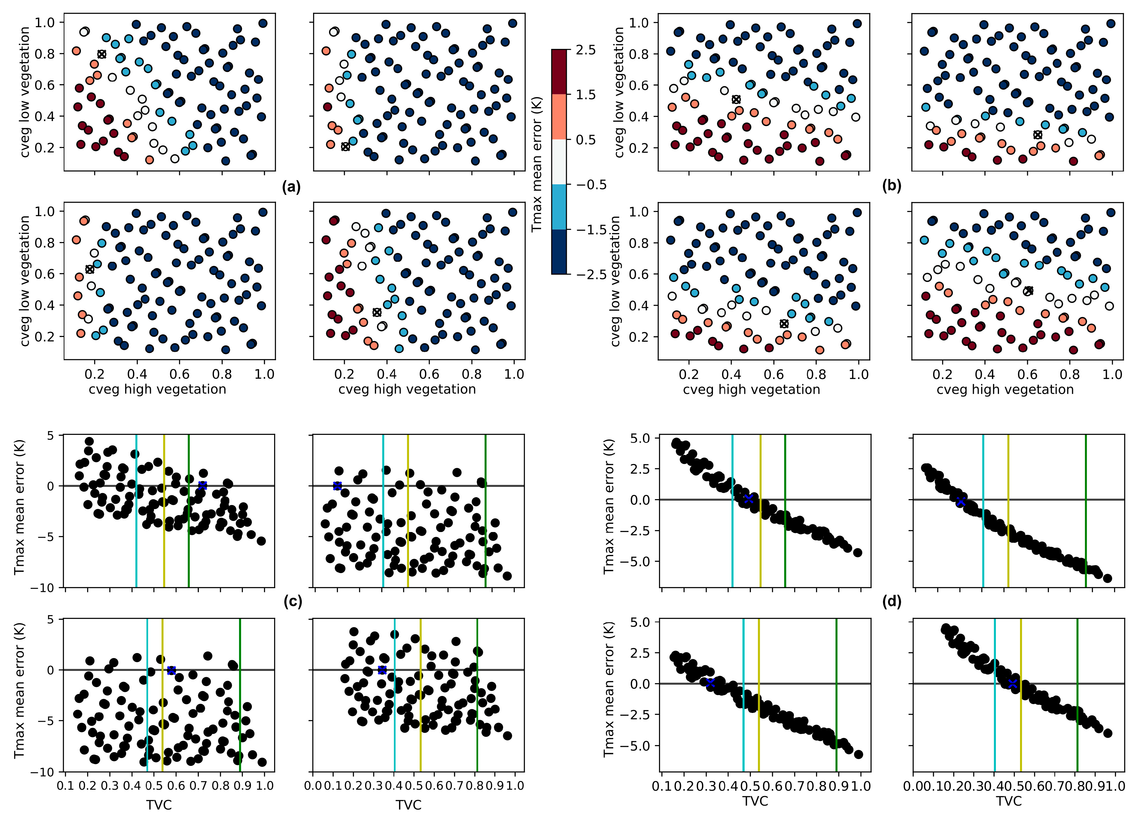
Chigh = CVHL × cveg(TVH)
Cbare = 1 − Clow − Chigh
TVC = Clow + Chigh
2.1.2. ECMWF’s Reanalyses
2.1.3. Simulations Setup
2.1.4. LSA-SAF’s Land Surface Temperature
2.1.5. Land Cover and Vegetation Datasets
2.2. Methods
2.2.1. Simulations Evaluation
- The reanalysis’ TCC < 0.3;
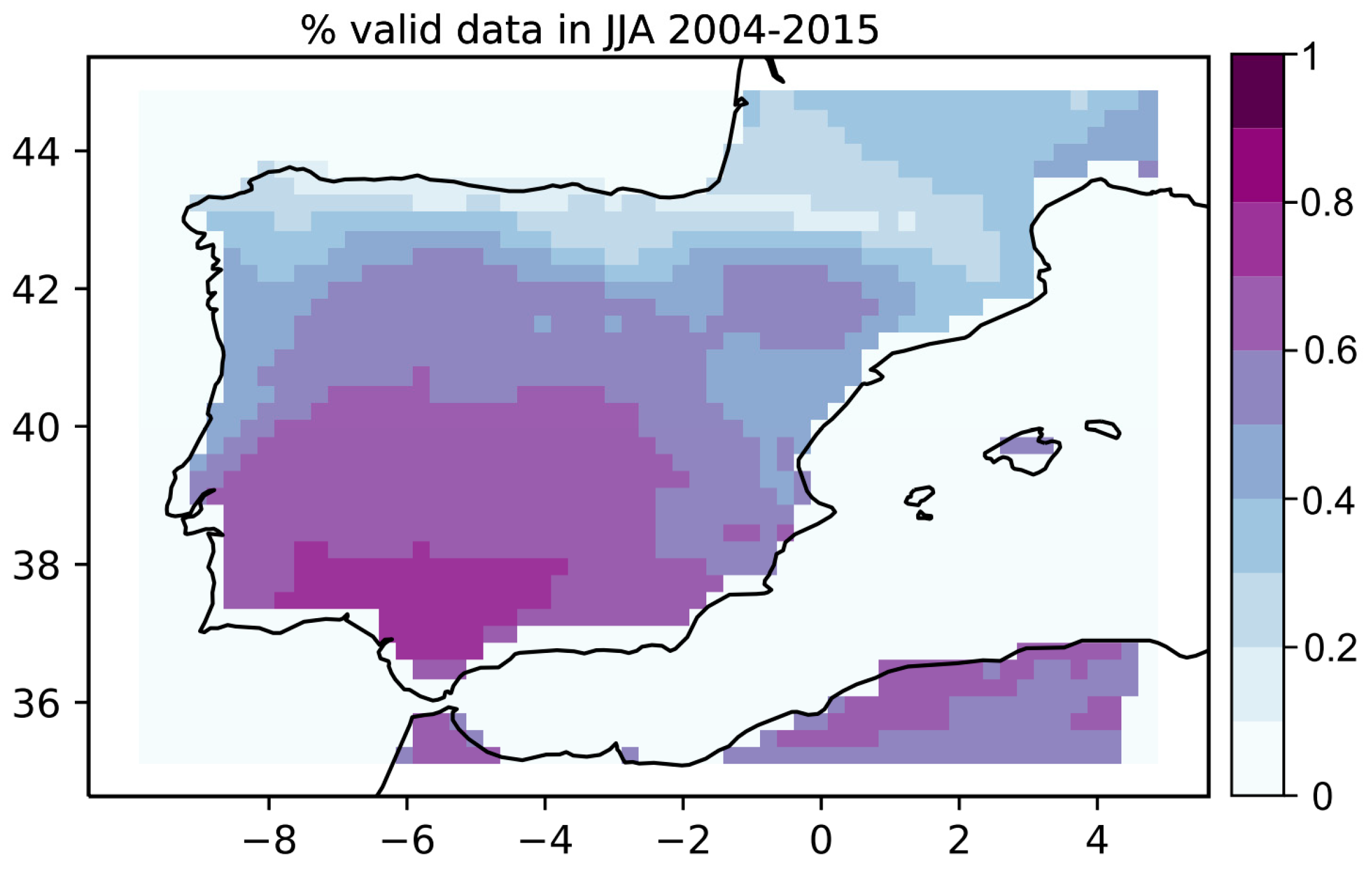
- The fraction of valid satellite LST original data in each 0.25° × 0.25° grid cell > 0.7.
- Tmax: 11 h–15 h;
- Tmin: 3 h–7 h.
2.2.2. Sensitivity Simulations
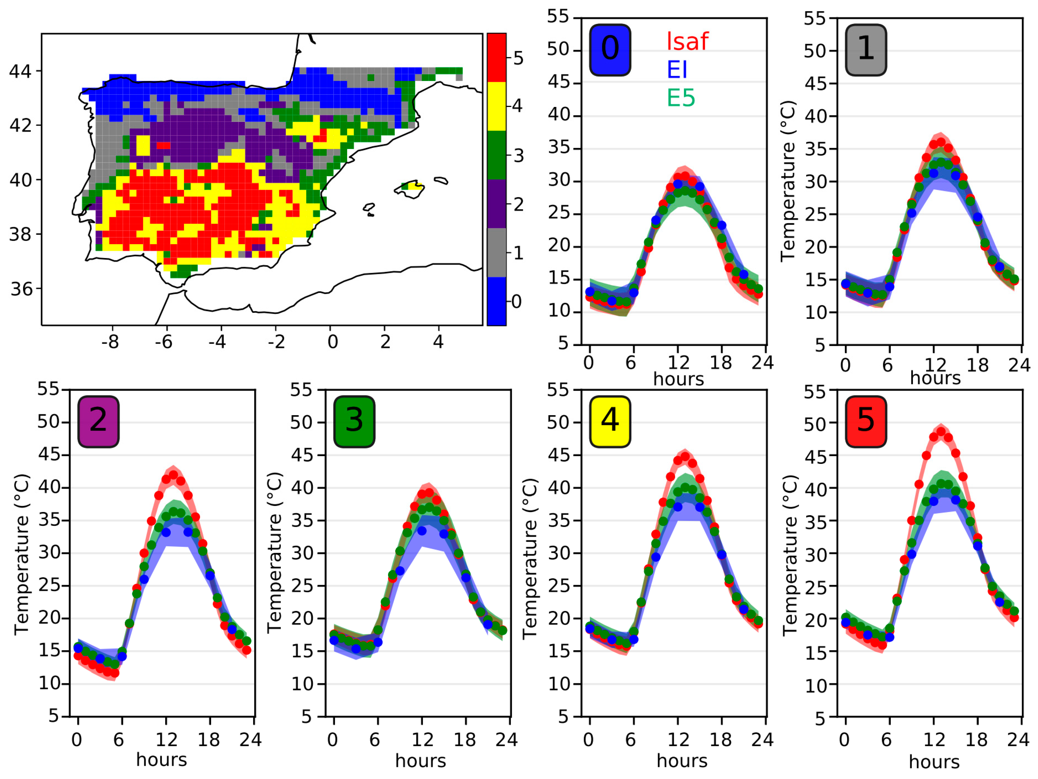
3. Results
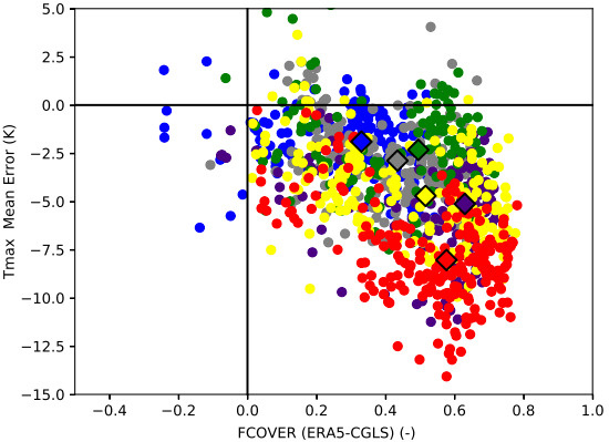
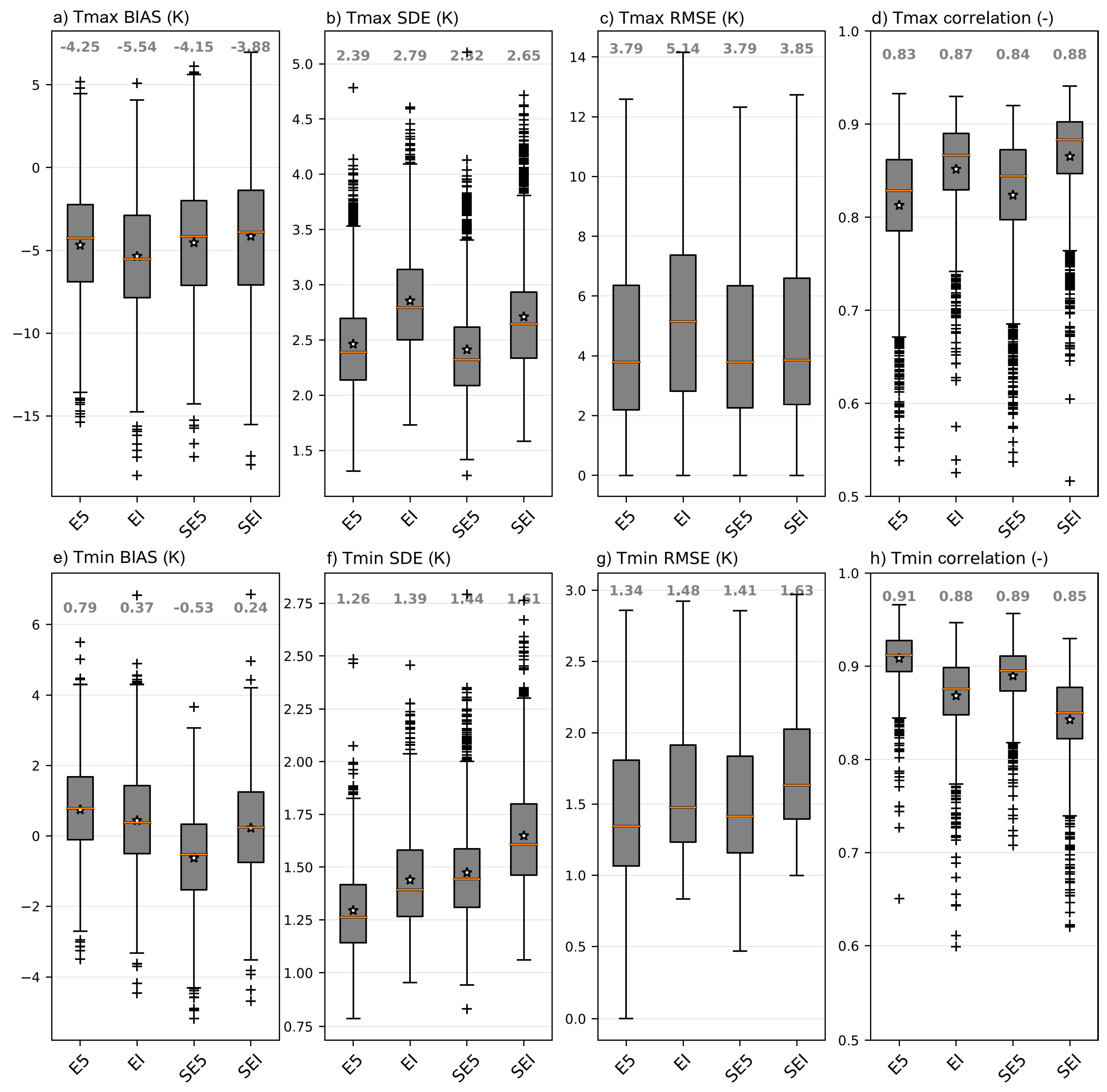
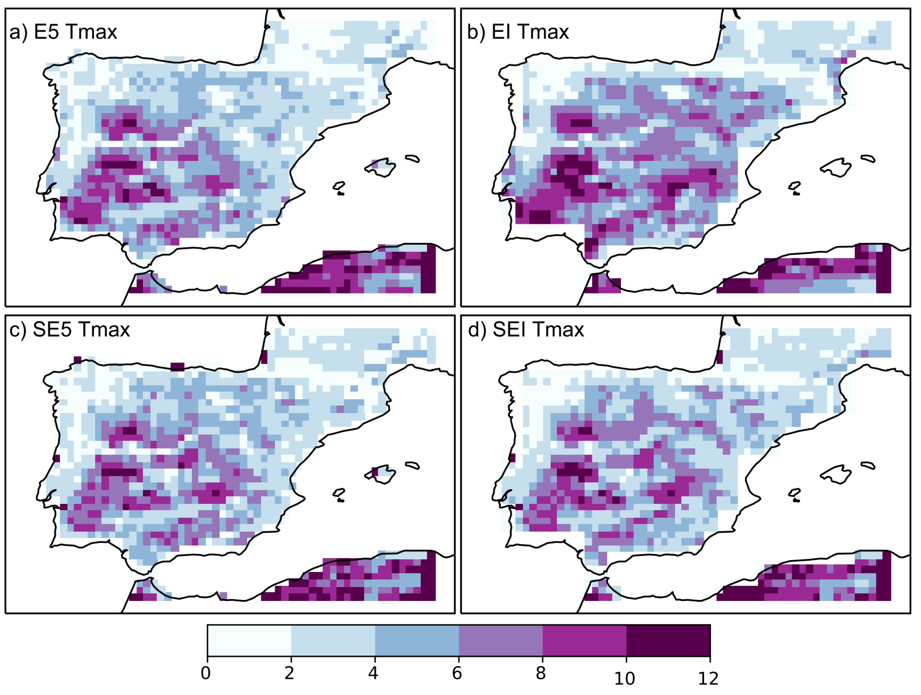
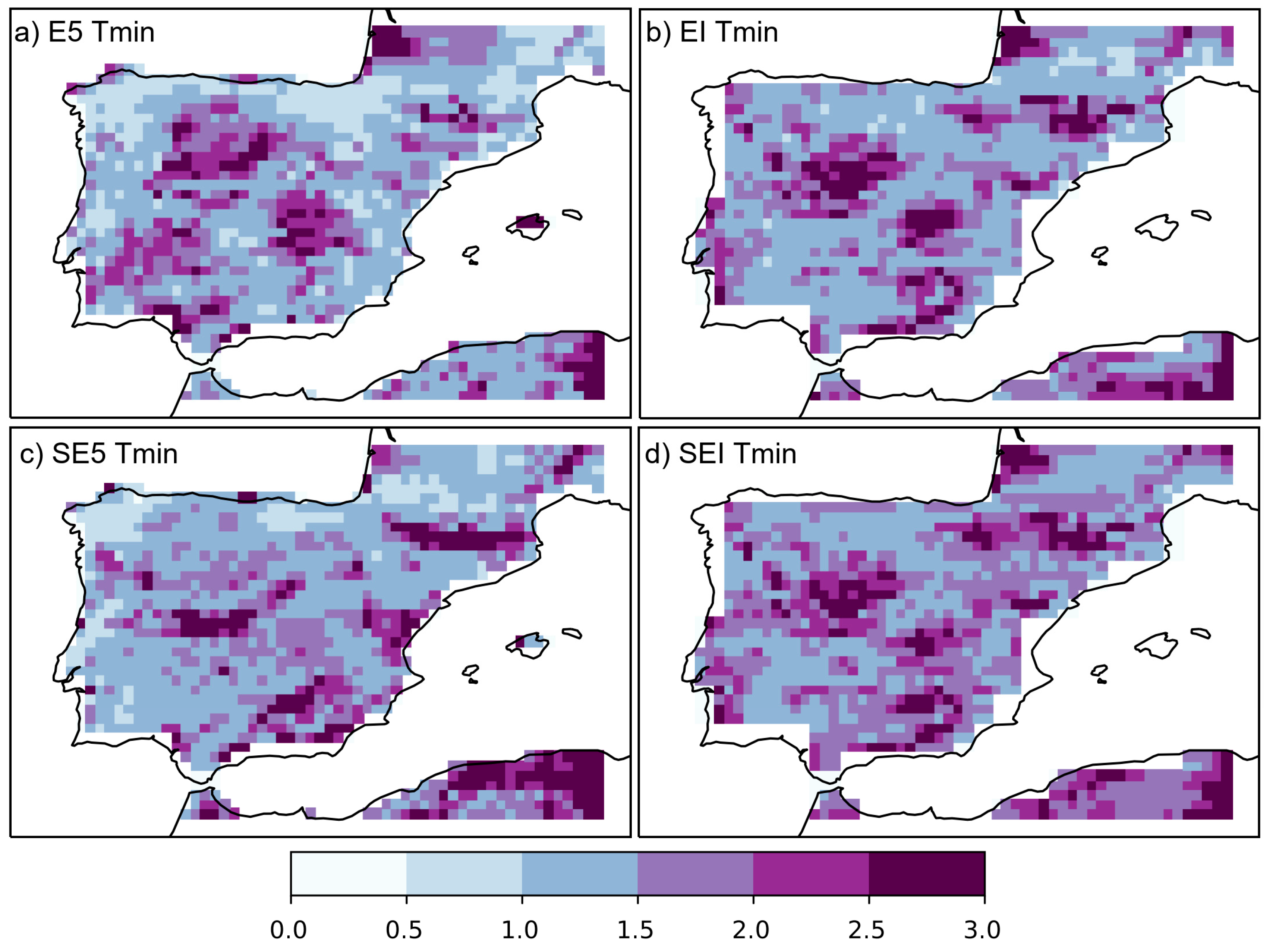
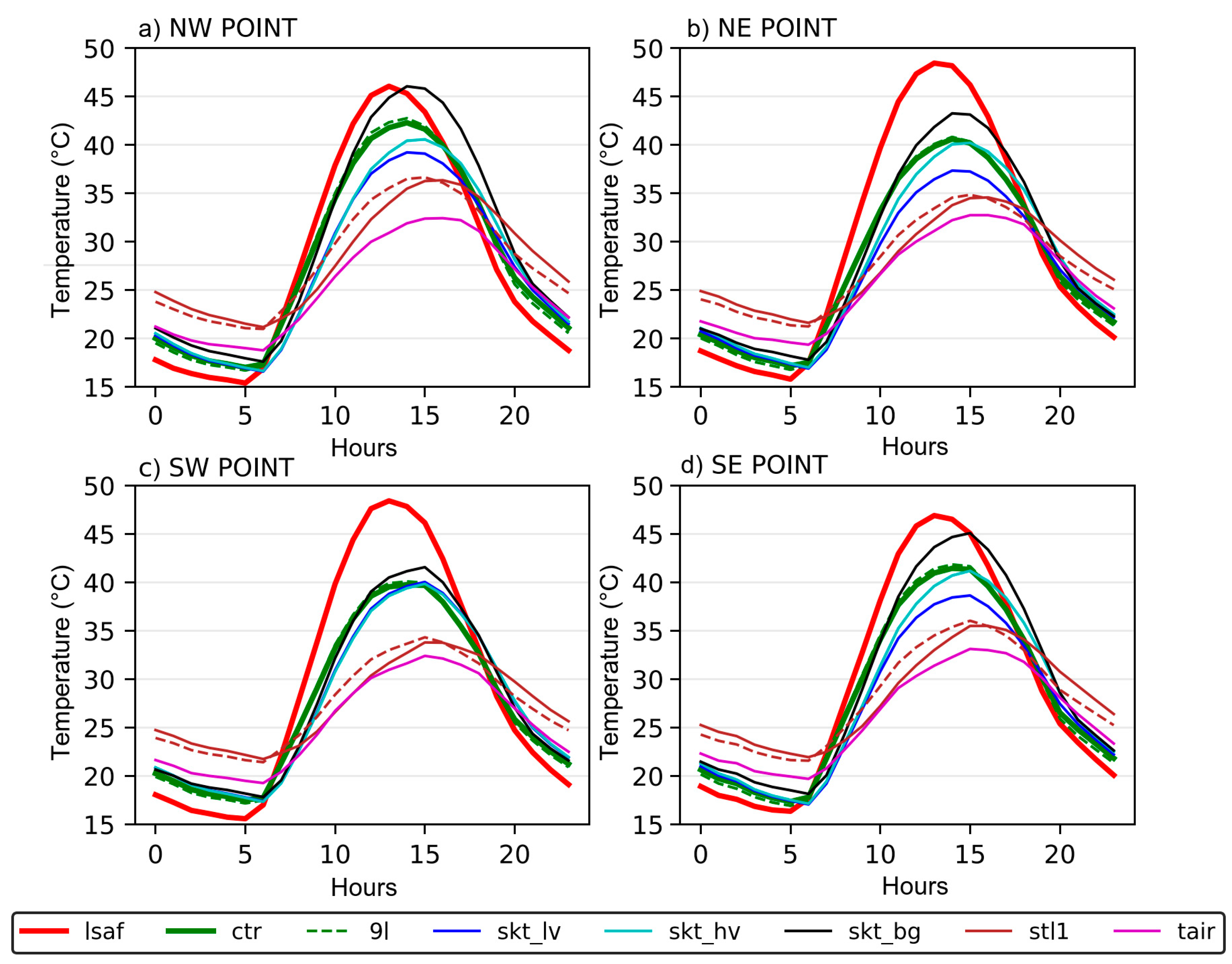
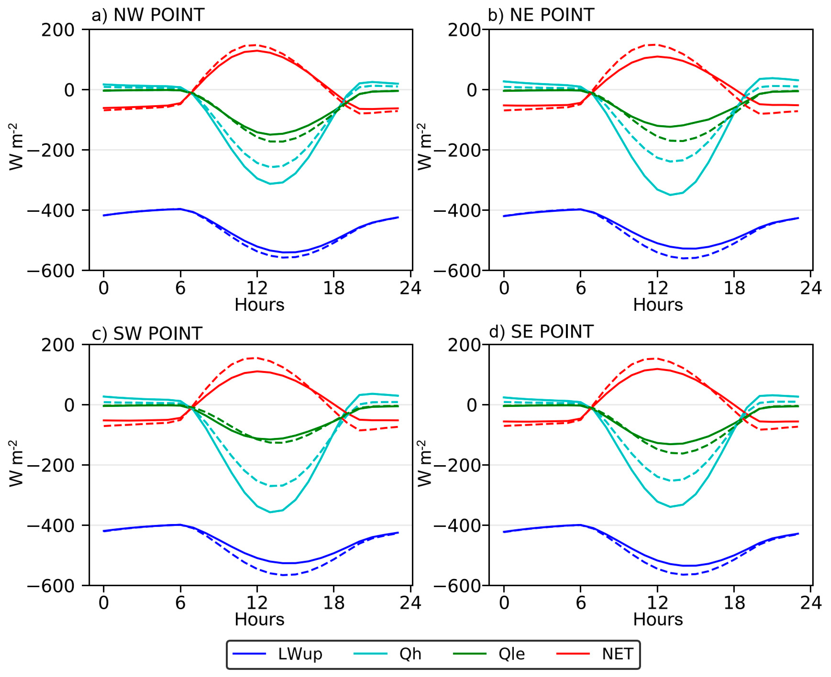
3.1. Evaluation
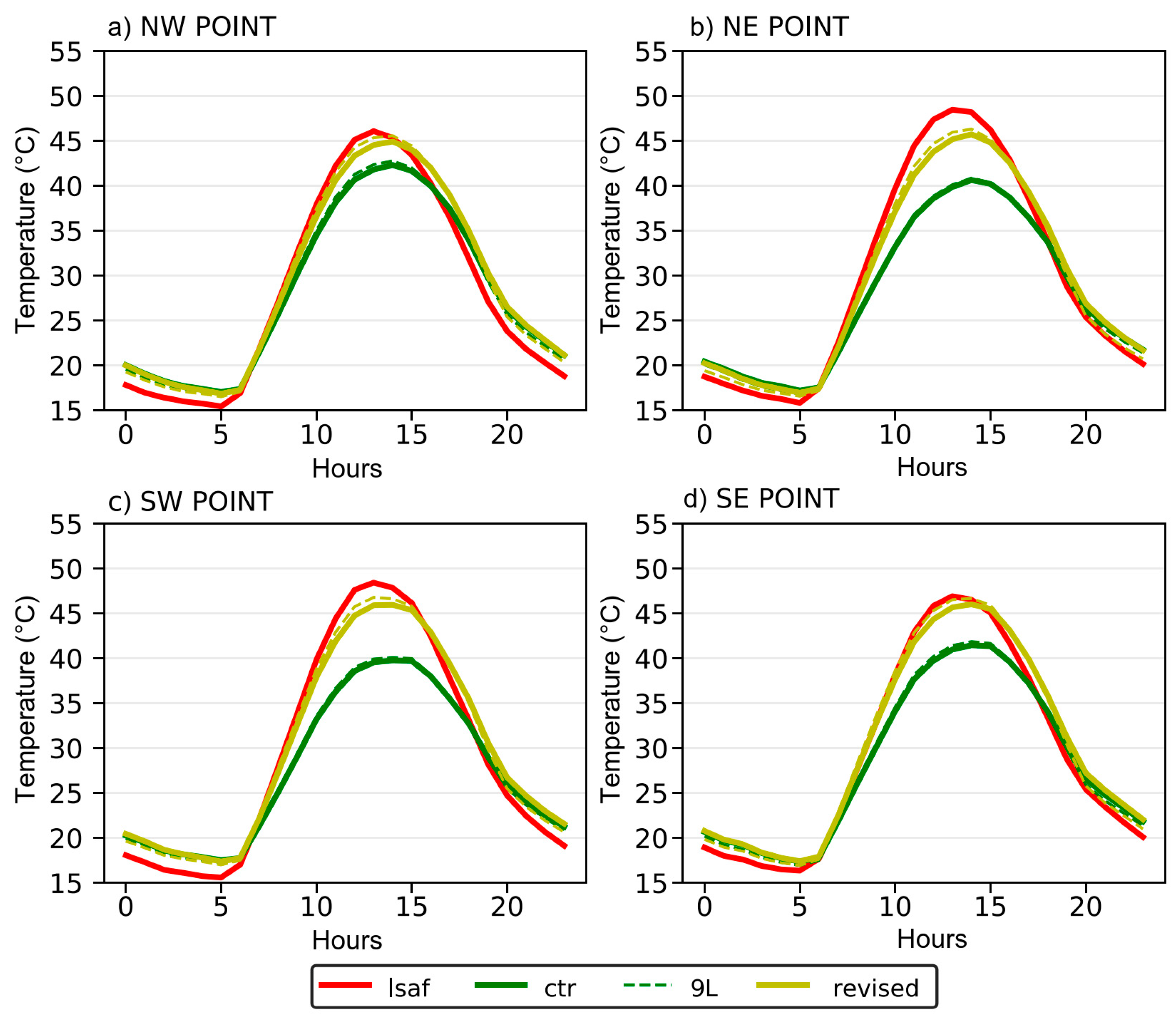
3.2. Sensitivity Experiments
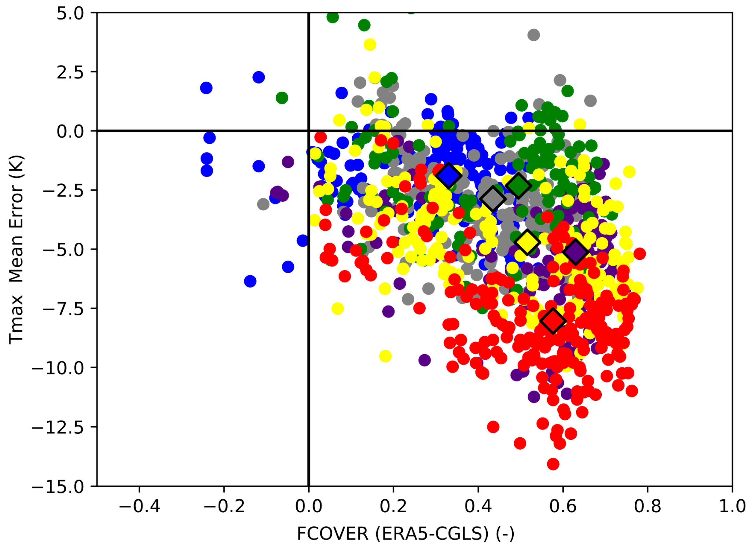
3.2.1. Vegetation Cover
3.2.2. Vegetation Type
4. Discussion
5. Conclusions
Supplementary Materials
Author Contributions
Funding
Acknowledgments
Conflicts of Interest
References
- Bojinski, S.; Verstraete, M.; Peterson, T.C.; Richter, C.; Simmons, A.; Zemp, M. The Concept of Essential Climate Variables in Support of Climate Research, Applications, and Policy. Bull. Am. Meteorol. Soc. 2014, 95, 1431–1443. [Google Scholar] [CrossRef]
- Li, Z.-L.; Tang, B.-H.; Wu, H.; Ren, H.; Yan, G.; Wan, Z.; Trigo, I.F.; Sobrino, J.A. Satellite-derived land surface temperature: Current status and perspectives. Remote Sens. Environ. 2013, 131, 14–37. [Google Scholar] [CrossRef]
- Norman, J.M.; Becker, F. Terminology in thermal infrared remote sensing of natural surfaces. Agric. Meteorol. 1995, 77, 153–166. [Google Scholar] [CrossRef]
- Holmes, T.R.H.; De Jeu, R.A.M.; Owe, M.; Dolman, A.J. Land surface temperature from Ka band (37 GHz) passive microwave observations. J. Geophys. Res. 2009, 114, 2005. [Google Scholar] [CrossRef]
- Zheng, W.; Wei, H.; Wang, Z.; Zeng, X.; Meng, J.; Ek, M.; Mitchell, K.; Derber, J. Improvement of daytime land surface skin temperature over arid regions in the NCEP GFS model and its impact on satellite data assimilation: LST IMPROVEMENT AND DATA ASSIMILATION. J. Geophys. Res. 2012, 117. [Google Scholar] [CrossRef]
- Zhou, L.; Dickinson, R.E.; Tian, Y.; Jin, M.; Ogawa, K.; Yu, H.; Schmugge, T. A sensitivity study of climate and energy balance simulations with use of satellite-derived emissivity data over Northern Africa and the Arabian Peninsula: EMISSIVITY AND CLIMATE MODELS. J. Geophys. Res. 2003, 108. [Google Scholar] [CrossRef]
- Trigo, I.F.; Boussetta, S.; Viterbo, P.; Balsamo, G.; Beljaars, A.; Sandu, I. Comparison of model land skin temperature with remotely sensed estimates and assessment of surface-atmosphere coupling. J. Geophys. Res. Atmos. 2015, 120, 12–96. [Google Scholar] [CrossRef]
- Orth, R.; Dutra, E.; Trigo, I.F.; Balsamo, G. Advancing land surface model development with satellite-based Earth observations. Hydrol. Earth Syst. Sci. 2017, 21, 2483–2495. [Google Scholar] [CrossRef]
- Hooker, J.; Duveiller, G.; Cescatti, A. A global dataset of air temperature derived from satellite remote sensing and weather stations. Sci. Data 2018, 5, 180246. [Google Scholar] [CrossRef]
- Good, E.J. An in situ-based analysis of the relationship between land surface “skin” and screen-level air temperatures: Land Skin-Air Temperature Relationship. J. Geophys. Res. Atmos. 2016, 121, 8801–8819. [Google Scholar] [CrossRef]
- Wan, Z.; Dozier, J. A generalized split-window algorithm for retrieving land-surface temperature from space. IEEE Trans. Geosci. Remote Sens. 1996, 34, 892–905. [Google Scholar]
- Becker, F.; Li, Z.-L. Towards a local split window method over land surfaces. Int. J. Remote Sens. 1990, 11, 369–393. [Google Scholar] [CrossRef]
- Trigo, I.F.; Dacamara, C.C.; Viterbo, P.; Roujean, J.-L.; Olesen, F.; Barroso, C.; Camacho-de-Coca, F.; Carrer, D.; Freitas, S.C.; García-Haro, J.; et al. The Satellite Application Facility for Land Surface Analysis. Int. J. Remote Sens. 2011, 32, 2725–2744. [Google Scholar] [CrossRef]
- Wan, Z. New refinements and validation of the collection-6 MODIS land-surface temperature/emissivity product. Remote Sens. Environ. 2014, 140, 36–45. [Google Scholar] [CrossRef]
- Freitas, S.C.; Trigo, I.F.; Macedo, J.; Barroso, C.; Silva, R.; Perdigão, R. Land surface temperature from multiple geostationary satellites. Int. J. Remote Sens. 2013, 34, 3051–3068. [Google Scholar] [CrossRef]
- Ermida, S.L.; Trigo, I.F.; DaCamara, C.C.; Jiménez, C.; Prigent, C. Quantifying the Clear-Sky Bias of Satellite Land Surface Temperature Using Microwave-Based Estimates. J. Geophys. Res. Atmos. 2019, 124, 844–857. [Google Scholar] [CrossRef]
- Schar, C.; Vidale, P.L.; Luthi, D.; Frei, C.; Haberli, C.; Liniger, M.A.; Appenzeller, C. The role of increasing temperature variability in European summer heatwaves. Nature 2004, 427, 332–336. [Google Scholar] [CrossRef]
- Seneviratne, S.I.; Luthi, D.; Litschi, M.; Schar, C. Land-atmosphere coupling and climate change in Europe. Nature 2006, 443, 205–209. [Google Scholar] [CrossRef]
- Dirmeyer, P.A.; Chen, L.; Wu, J.; Shin, C.-S.; Huang, B.; Cash, B.A.; Bosilovich, M.G.; Mahanama, S.; Koster, R.D.; Santanello, J.A.; et al. Verification of land-atmosphere coupling in forecast models, reanalyses and land surface models using flux site observations. J. Hydrometeorol. 2018, 19, 375–392. [Google Scholar] [CrossRef]
- Ukkola, A.M.; Kauwe, M.G.D.; Pitman, A.J.; Best, M.J.; Abramowitz, G.; Haverd, V.; Decker, M.; Haughton, N. Land surface models systematically overestimate the intensity, duration and magnitude of seasonal-scale evaporative droughts. Environ. Res. Lett. 2016, 11, 104012. [Google Scholar] [CrossRef]
- Kala, J.; De Kauwe, M.G.; Pitman, A.J.; Medlyn, B.E.; Wang, Y.-P.; Lorenz, R.; Perkins-Kirkpatrick, S.E. Impact of the representation of stomatal conductance on model projections of heatwave intensity. Sci. Rep. 2016, 6, 23418. [Google Scholar] [CrossRef] [PubMed]
- Best, M.J.; Abramowitz, G.; Johnson, H.R.; Pitman, A.J.; Balsamo, G.; Boone, A.; Cuntz, M.; Decharme, B.; Dirmeyer, P.A.; Dong, J.; et al. The Plumbing of Land Surface Models: Benchmarking Model Performance. J. Hydrometeorol. 2015, 16, 1425–1442. [Google Scholar] [CrossRef]
- Haughton, N.; Abramowitz, G.; Pitman, A.J.; Or, D.; Best, M.J.; Johnson, H.R.; Balsamo, G.; Boone, A.; Cuntz, M.; Decharme, B.; et al. The Plumbing of Land Surface Models: Is Poor Performance a Result of Methodology or Data Quality? J. Hydrometeorol. 2016, 17, 1705–1723. [Google Scholar] [CrossRef] [PubMed]
- Dee, D.P.; Uppala, S.M.; Simmons, A.J.; Berrisford, P.; Poli, P.; Kobayashi, S.; Andrae, U.; Balmaseda, M.A.; Balsamo, G.; Bauer, P.; et al. The ERA-Interim reanalysis: Configuration and performance of the data assimilation system. QJR Meteorol. Soc. 2011, 137, 553–597. [Google Scholar] [CrossRef]
- Hersbach, H.; de Rosnay, P.; Bell, B.; Schepers, D.; Simmons, A.; Soci, C.; Abdalla, S.; Alonso-Balmaseda, M.; Balsamo, G.; Bechtold, P.; et al. Operational Global Reanalysis: Progress, Future Directions and Synergies with NWP. ECMWF Re-Anal. Proj. Rep. Ser. 2018, 27, 1–63. [Google Scholar]
- Balsamo, G.; Boussetta, S.; Dutra, E.; Beljaars, A.; Viterbo, P.; Van den Hurk, B. Evolution of land surface processes in the IFS. ECMWF Newsl. 2011, 127, 17–22. [Google Scholar]
- Balsamo, G.; Albergel, C.; Beljaars, A.; Boussetta, S.; Brun, E.; Cloke, H.; Dee, D.; Dutra, E.; Muñoz-Sabater, J.; Pappenberger, F.; et al. ERA-Interim/Land: A global land surface reanalysis data set. Hydrol. Earth Syst. Sci. 2015, 19, 389–407. [Google Scholar] [CrossRef]
- Albergel, C.; Dutra, E.; Munier, S.; Calvet, J.-C.; Munoz-Sabater, J.; de Rosnay, P.; Balsamo, G. ERA-5 and ERA-Interim driven ISBA land surface model simulations: Which one performs better? Hydrol. Earth Syst. Sci. 2018, 22, 3515–3532. [Google Scholar] [CrossRef]
- Zhou, C.; Wang, K.; Ma, Q. Evaluation of Eight Current Reanalyses in Simulating Land Surface Temperature from 1979 to 2003 in China. J. Clim. 2017, 30, 7379–7398. [Google Scholar] [CrossRef]
- Ghent, D.; Kaduk, J.; Remedios, J.; Ardö, J.; Balzter, H. Assimilation of land surface temperature into the land surface model JULES with an ensemble Kalman filter. J. Geophys. Res. 2010, 115, GB1008. [Google Scholar] [CrossRef]
- ECMWF (Ed.) Part IV: Physical Processes. In IFS Documentation CY45R1; ECMWF: Reading, UK, 2018. [Google Scholar]
- Loveland, T.R.; Reed, B.C.; Brown, J.F.; Ohlen, D.O.; Zhu, Z.; Yang, L.; Merchant, J.W. Development of a global land cover characteristics database and IGBP DISCover from 1 km AVHRR data. Int. J. Remote Sens. 2000, 21, 1303–1330. [Google Scholar] [CrossRef]
- Hersbach, H.; Bell, W.; Berrisford, P.; Horányi, A.; Joaquí, M.-S.; Nicolas, J.; Radu, R.; Schepers, D.; Simmons, A.; Soci, C.; et al. Global Reanalysis: Goodbye ERA-Interim, Hello ERA5. ECMWF Newsl. 2019, 159, 17–24. [Google Scholar]
- Verger, A.; Baret, F.; Weiss, M. Near Real-Time Vegetation Monitoring at Global Scale. IEEE J. Sel. Top. Appl. Earth Obs. Remote Sens. 2014, 7, 3473–3481. [Google Scholar] [CrossRef]
- Poulter, B.; MacBean, N.; Hartley, A.; Khlystova, I.; Arino, O.; Betts, R.; Bontemps, S.; Boettcher, M.; Brockmann, C.; Defourny, P.; et al. Plant functional type classification for earth system models: Results from the European Space Agency’s Land Cover Climate Change Initiative. Geosci. Model. Dev. 2015, 8, 2315–2328. [Google Scholar] [CrossRef]
- Hartigan, J.A. Clustering Algorithms, 99th ed.; John Wiley & Sons Inc.: New York, NY, USA, 1975; ISBN 978-0-471-35645-5. [Google Scholar]
- Dorigo, W.; Wagner, W.; Albergel, C.; Albrecht, F.; Balsamo, G.; Brocca, L.; Chung, D.; Ertl, M.; Forkel, M.; Gruber, A.; et al. ESA CCI Soil Moisture for improved Earth system understanding: State-of-the art and future directions. Remote Sens. Environ. 2017, 203, 185–215. [Google Scholar] [CrossRef]
- Sobol’, I.M. On the distribution of points in a cube and the approximate evaluation of integrals. USSR Comput. Math. Math. Phys. 1967, 7, 86–112. [Google Scholar] [CrossRef]
- Orth, R.; Dutra, E.; Pappenberger, F. Improving Weather Predictability by Including Land Surface Model Parameter Uncertainty. Mon. Weather Rev. 2016, 144, 1551–1569. [Google Scholar] [CrossRef]
- Alessandri, A.; Catalano, F.; De Felice, M.; Van Den Hurk, B.; Doblas Reyes, F.; Boussetta, S.; Balsamo, G.; Miller, P.A. Multi-scale enhancement of climate prediction over land by increasing the model sensitivity to vegetation variability in EC-Earth. Clim. Dyn. 2017, 49, 1215–1237. [Google Scholar] [CrossRef]


| Index | Land Cover Type | H/L | Cveg | z0m | z0h |
|---|---|---|---|---|---|
| 1 | Crops, mixed farming | L | 0.90 | 0.25 | 0.25 × 10⁻² |
| 2 | Short grass | L | 0.85 | 0.20 | 0.20 × 10⁻² |
| 3 | Evergreen needleleaf trees | H | 0.90 | 2.00 | 2.00 |
| 4 | Deciduous needleleaf trees | H | 0.90 | 2.00 | 2.00 |
| 5 | Deciduous broadleaf trees | H | 0.90 | 2.00 | 2.00 |
| 6 | Evergreen broadleaf trees | H | 0.99 | 2.00 | 2.00 |
| 7 | Tall grass | L | 0.70 | 0.47 | 0.47 × 10⁻² |
| 8 | Desert | - | 0 | 0.013 | 0.013 × 10⁻² |
| 9 | Tundra | L | 0.50 | 0.034 | 0.034 × 10⁻² |
| 10 | Irrigated crops | L | 0.90 | 0.50 | 0.50 × 10⁻² |
| 11 | Semidesert | L | 0.1 | 0.17 | 0.17 × 10⁻² |
| 12 | Ice caps and glaciers | - | - | 1.3 × 10⁻³ | 1.3 × 10⁻⁴ |
| 13 | Bogs and marshes | L | 0.6 | 0.83 | 0.83 × 10⁻² |
| 14 | Inland water | - | - | - | - |
| 15 | Ocean | - | - | - | - |
| 16 | Evergreen shrubs | L | 0.50 | 0.10 | 0.10 × 10⁻² |
| 17 | Deciduous shrubs | L | 0.50 | 0.25 | 0.25 × 10⁻² |
| 18 | Mixed forest | H | 0.90 | 2.00 | 2.00 |
| 19 | Interrupted forest | H | 0.90 | 1.1 | 1.1 |
| 20 | Water and land mixtures | L | 0.60 | - | - |
| Experiment | CVL | CVH | cveg | TVC |
|---|---|---|---|---|
| CTR,9L (SEI 1, SE5 1) | IFS 2 | IFS 2 | Table 1 | Equation (1) |
| bare | 0 | 0 | ||
| lveg | IFS 2 | 0 | ||
| hveg | 0 | IFS 2 | ||
| nlveg | CGLS-FCover | 0 | 1 | CGLS-FCover |
| nhveg | 0 | CGLS-FCover | 1 | |
| revised | ESA-CCI 3 | ESA-CCI 3 | Table 1 | Equation (1) |
| Point | CVL | CVH | IFS TVC | CGLS FCover |
|---|---|---|---|---|
| NW | 0.87 (0.40) | 0.13 (0.51) | 0.55 (0.66) | 0.42 |
| NE | 0.89 (0.07) | 0.08 (0.93) | 0.52 (0.87) | 0.41 |
| SW | 0.89 (0.01) | 0.10 (0.99) | 0.54 (0.89) | 0.47 |
| SE | 0.85 (0.17) | 0.12 (0.81) | 0.53 (0.81) | 0.40 |
© 2019 by the authors. Licensee MDPI, Basel, Switzerland. This article is an open access article distributed under the terms and conditions of the Creative Commons Attribution (CC BY) license (http://creativecommons.org/licenses/by/4.0/).
Share and Cite
Johannsen, F.; Ermida, S.; Martins, J.P.A.; Trigo, I.F.; Nogueira, M.; Dutra, E. Cold Bias of ERA5 Summertime Daily Maximum Land Surface Temperature over Iberian Peninsula. Remote Sens. 2019, 11, 2570. https://doi.org/10.3390/rs11212570
Johannsen F, Ermida S, Martins JPA, Trigo IF, Nogueira M, Dutra E. Cold Bias of ERA5 Summertime Daily Maximum Land Surface Temperature over Iberian Peninsula. Remote Sensing. 2019; 11(21):2570. https://doi.org/10.3390/rs11212570
Chicago/Turabian StyleJohannsen, Frederico, Sofia Ermida, João P. A. Martins, Isabel F. Trigo, Miguel Nogueira, and Emanuel Dutra. 2019. "Cold Bias of ERA5 Summertime Daily Maximum Land Surface Temperature over Iberian Peninsula" Remote Sensing 11, no. 21: 2570. https://doi.org/10.3390/rs11212570
APA StyleJohannsen, F., Ermida, S., Martins, J. P. A., Trigo, I. F., Nogueira, M., & Dutra, E. (2019). Cold Bias of ERA5 Summertime Daily Maximum Land Surface Temperature over Iberian Peninsula. Remote Sensing, 11(21), 2570. https://doi.org/10.3390/rs11212570