Pixel-Wise PolSAR Image Classification via a Novel Complex-Valued Deep Fully Convolutional Network

Abstract

Although complex-valued (CV) neural networks have shown better classification results compared to their real-valued (RV) counterparts for polarimetric synthetic aperture radar (PolSAR) classification, the extension of pixel-level RV networks to the complex domain has not yet thoroughly examined. This paper presents a novel complex-valued deep fully convolutional neural network (CV-FCN) designed for PolSAR image classification. Specifically, CV-FCN uses PolSAR CV data that includes the phase information and uses the deep FCN architecture that performs pixel-level labeling. The CV-FCN architecture is trained in an end-to-end scheme to extract discriminative polarimetric features, and then the entire PolSAR image is classified by the trained CV-FCN. Technically, for the particularity of PolSAR data, a dedicated complex-valued weight initialization scheme is proposed to initialize CV-FCN. It considers the distribution of polarization data to conduct CV-FCN training from scratch in an efficient and fast manner. CV-FCN employs a complex downsampling-then-upsampling scheme to extract dense features. To enrich discriminative information, multi-level CV features that retain more polarization information are extracted via the complex downsampling scheme. Then, a complex upsampling scheme is proposed to predict dense CV labeling. It employs the complex max-unpooling layers to greatly capture more spatial information for better robustness to speckle noise. The complex max-unpooling layers upsample the real and the imaginary parts of complex feature maps based on the max locations maps retained from the complex downsampling scheme. In addition, to achieve faster convergence and obtain more precise classification results, a novel average cross-entropy loss function is derived for CV-FCN optimization. Experiments on real PolSAR datasets demonstrate that CV-FCN achieves better classification performance than other state-of-art methods.

1. Introduction

Polarimetric synthetic aperture radar (PolSAR) images have received a lot of attention as they can provide more comprehensive and abundant information compared with SAR images [1]. In recent decades, the application of PolSAR images has received sustained development in the remote sensing field. In particular, land use land cover (LULC) classification is one of the most typical and important applications in automatic image analysis and interpretation [2]. Until now, numerous traditional schemes have been put forward for PolSAR image classification, such as Wishart classifiers [3,4,5], target decompositions (TDs) [6,7,8,9] and random fields (RFs) [10,11,12]. Those traditional methods often use some low-level or mid-level features, which are usually extracted by some feature extraction techniques. Generally, the extracted features include statistic features [5,10], backscattering elements [13], TDs-based features [8,9] as well as some popular features used for other images [14,15,16,17,18]. However, the extracted features are not only mostly class-specific and hand-crafted but also involve a considerable amount of manual trial and error [2]. Moreover, some extracted features such as TDs features rely heavily on the complex analysis of PolSAR data. Meanwhile, the selection of descriptive feature sets often increases computation time.

With the rapid development of learning algorithms, several machine learning tools do perform feature learning (or at least feature optimization), such as support vector machines (SVMs) [15,19] and random forest (RF) [2]. However, they are still shallow models that focus on many input features and may not be robust to nonlinear data [20]. Recently, deep learning (DL) methods represented by the deep convolutional neural networks (CNNs) have demonstrated remarkable learning ability in many image analysis fields [13,21,22,23]. With the rapid development of DL, many deep networks have been developed for the semantic segmentation, such as sparse autoencoder (SAE), deep fully convolutional neural network (FCN), deep belief network (DBN), generative adversarial network (GAN), and graph convolutional networks (GCN). Compared with the aforementioned conventional methods, DL techniques can automatically learn discriminative features and perform advanced tasks by multiple neural layers in an end-to-end manner, thereby reducing manual error and achieving promising results [23,24]. In recent years, some better DL-based algorithms have significantly improved the performance of PolSAR image classification. De et al. [25] proposed a classification scheme of urban areas in PolSAR data based on polarization orientation angle (POA) shifts and the SAE. Liu et al. [26] proposed the Wishart DBN (W-DBN) for PolSAR image classification. They defined the Wishart-Bernoulli restricted Boltzmann machine (WBRBM), and stacked WBRBM and binary RBM to form the W-DBN. Zhou et al. [27] introduced CNN for PolSAR image classification to automatically learn hierarchical polarimetric spatial features. Bin et al. [28] improved a CNN model and presented a graph-based semisupervised CNN for PolSAR image classification. Inspired by the success of FCN, Wang et al. [29] presented an effective PolSAR image classification scheme to integrate deep spatial patterns learned automatically by FCN. Li et al. [30] proposed the sliding window FCN and sparse coding (SFCN-SC) for PolSAR image classification. They employed sliding window operation to apply the FCN architecture directly to PolSAR images. Mohammadimanesh et al. [31] specially designed a new FCN architecture for the classification of wetland complexes using PolSAR imagery. Furthermore, Pham et al. [32] employed the SegNet model for the classification of very high resolution (VHR) PolSAR data. However, most studies on DL methods for PolSAR classification tasks predominantly focus on the case of real-valued neural networks (RV-NNs).

Notably, in RV-NNs, inputs, weights, and outputs are all modeled as real-valued (RV) numbers. This means that projections are required to convert the PolSAR complex-valued (CV) data to RV features as RV-NNs input. Although RV-NNs have demonstrated excellent performance in PolSAR image classification tasks, there are a couple of problems stated by RV features. First, it is unclear which projection yields the best performance towards a particular PolSAR image. Although the descriptive feature set generated by multi-projection has achieved remarkable results, a larger feature set means larger computation time and memory consumption, and may even cause data redundancy problems [2]. Secondly, projection sometimes means a loss of valuable information, especially the phase information, which may lead to unsatisfactory results. Actually, the phase of multi-channel SAR data can provide useful information in the interpretation of SAR images. Especially for PolSAR systems, the phase differences between polarizations have received significant attention for a couple of decades [33,34,35].

In view of the aforementioned problems, some researchers have begun to investigate networks which are tailored to CV data of PolSAR images rather than requiring any projection to classify PolSAR images. Hansch et al. [36] first proposed the complex-valued MLPs (CV-MLPs) for land use classification in PolSAR images. Shang et al. [37] suggested a complex-valued feedforward neural network in the Poincare sphere parameter space. Moreover, an improved quaternion neural network [38] and a quaternion autoencoder [39] have been proposed for PolSAR land classification. Recently, a complex-valued CNN (CV-CNN) specifically designed for PolSAR image classification has been proposed by Zhang et al. [40], where the authors derived a complex backpropagation algorithm based on stochastic gradient descent for CV-CNN training.

Although CV-NNs have achieved remarkable breakthroughs for PolSAR image classification, they still suffer some challenges. First, we find that relatively deep network architectures have not received considerable attention in the complex domain. The structures of the above CV-NNs are relatively simple with limited feature extraction layers. This results in limited learning characteristics, which may yield the risk of sub-optimal classification results. Secondly, these networks fail to sufficiently take spatial information into account to effectively reduce the impact of speckles on classification results. Due to the inherent existence of speckle in PolSAR images, the pixel-based classification is easily affected and even leads to incorrect results. In this case, these CV-NNs would be ineffective to explicitly distinguish complex classes, since only local contexts caused by small image patches are considered. Thirdly, it is necessary to construct a CV-NN for direct pixel-wise labeling to predict fast and effectively. Actually, the image classification is a dense (pixel-level) problem that aims at assigning a label to each pixel in the input image. However, existing CV-NNs usually assign an entire input image patch to a category. This results in a large amount of redundant processing and leads to serious repetitive computation.

In response to the above challenges, this paper explores a complex-valued deep FCN architecture, which is an extension of FCN to the complex domain. The FCN is first proposed in [41] and is an excellent pixel-level classifier for semantic labeling. Typically, FCN outputs a 2-dimensional (2D) spatial image and can preserve certain spatial context information for accurate labeling results. Recently, FCNs have demonstrated remarkable classification ability in the remote sensing community [42,43]. However, to use FCN in the complex domain (i.e., CV-FCN) for PolSAR image classification, some tricky problems need to be tackled. First, the CV-FCN tailored to PolSAR data requires a proper scheme for the initialization of complex-valued weights. Generally, FCNs are often pre-trained on VGG-16 [44], whose parameters are first trained using optical images and are all real-valued numbers. However, those parameters are not appropriate to initialize CV weights of CV-FCN and are ineffective for PolSAR images since they cannot preserve polarimetric phase information. Therefore, a proper complex-valued weight initialization scheme not only can effectively initialize CV weights but also has the potential to reduce the risks of vanishing or exploding gradients, thereby speeding up the training process and improving the performance of networks. Secondly, layers in the upsampling scheme of CV-FCN should be constructed in the complex domain. Although some works have extended some layers to the complex domain [36,40,45], upsampling layers have not yet thoroughly examined in such domain. Finally, it is necessary to select a loss function for predicted CV labeling in the training processing of CV-FCN. The aim is to achieve faster convergence during CV-FCN optimization and obtain higher classification accuracy. Thus, how to design a reasonable loss function in the complex domain that is suitable for PolSAR images classification needs to be solved.

In view of the above-involved limitations, we present a novel complex-valued deep fully convolutional network (CV-FCN) for the classification of PolSAR imagery. The proposed deep CV-FCN adopts the complex downsampling-then-upsampling scheme to achieve pixel-wise classification results. To this end, this paper focuses on four works: (1) complex-valued weight initialization for faster PolSAR feature learning; (2) multi-level CV feature extraction for enriching discriminative information; (3) more spatial information recovery for stronger speckle noise immunity; (4) average cross-entropy loss function for more precise labeling results. Specifically, CV weights of CV-FCN are first initialized by a new complex-valued weight initialization scheme. The scheme explicitly focuses on the statistical characteristics of PolSAR data. Thus, it is very effective for faster training. Then, different-level CV features that retain more polarization information are extracted via the complex downsampling section. Those CV features have a powerful discriminative capacity for various classes. Subsequently, the complex upsampling section upsamples low-resolution CV feature maps and generates dense labeling. Notably, for more spatial information retaining, the complex max-unpooling layers are used in the upsampling section. Those layers recover more spatial information by the max locations maps to reduce the effect of speckles on coherent labeling results as well as improve boundary delineation. In addition, to promote CV-FCN training more effectively, an average cross-entropy loss function is employed in the process of updating CV-FCN parameters. The loss function performs the cross-entropy operation on the real and imaginary parts of CV predicted labeling, respectively. In this way, the phase information is also taken into account during parameter updating, which makes the classification of PolSAR images more precise. Extensive experimental results reflect the effectiveness of CV-FCN for the classification of PolSAR imagery. In summary, the major contributions of this paper can be highlighted as follows:

• The CV-FCN structure is proposed for PolSAR image classification, whose weights, biases, inputs, and outputs are all modeled as complex values. The CV-FCN directly uses raw PolSAR CV data as input without any data projection. In this case, it can extract multi-level and more robust CV features that retain more polarization information and have a powerful discriminative capacity for various categories.
• A new complex-valued weight initialization scheme is employed to initialize CV-FCN parameters. It allows CV-FCN to mine polarimetric features with relatively few adjustments. Thus, it can speed up CV-FCN training and save computation time.
• A complex upsampling scheme for CV-FCN is proposed to capture more spatial information through the complex max-unpooling layers. This scheme cannot only simplify the upsampling learning optimization but also recover more spatial information by max locations maps to reduce the impact of speckles. Thus, smoother and more coherent classification results can be achieved.
• A new average cross-entropy loss function in the complex domain is employed for CV-FCN optimization. It takes the phase information into account during parameters updating by average cross-entropy operation of predicted CV labels. Therefore, the new loss function enables CV-FCN optimization more precise while boosting the labeling accuracy.

The remainder of this paper is organized as follows. Section 2 formulates a detailed theory for the classification method of CV-FCN. In Section 3, the experiment results on real benchmark PolSAR images are reported. In addition, some related discussions are presented in Section 4. Finally, the conclusion and future works are given in Section 5.

2. Proposed Method

In this work, a deep CV-FCN is proposed to conduct the PolSAR image classification. The CV-FCN method integrates the feature extraction module and the classification module in a unified framework. Thus, features extracted through CV-FCN trained by PolSAR data are more able to distinguish various categories for PolSAR classification tasks. In the following, we first give the framework of the deep CV-FCN classification method in Section 2.1. Then, to learn more discriminative features for classification faster and more accurately, it is critical to train CV-FCN suitable for PolSAR images. Thus, we highlight and introduce four critical works for CV-FCN training in Section 2.2, Section 2.3 and Section 2.4. They include CV weight initialization, deep and multi-level CV feature extraction, more spatial information recovery, and loss function for more precise optimization. Finally, the CV-FCN classification algorithm is summarized in Section 2.5.

2.1. Framework of the Deep CV-FCN Classification Method

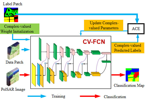
The framework of the CV-FCN classification method is shown in Figure 1, which consists of two separate modules: the feature extraction module and the classification module. In the feature extraction module, CV-FCN is trained to exploit the discriminative information. Then, the trained CV-FCN is used to classify PolSAR images in the classification module.

The data patches set and the corresponding label patches set are first prepared as input to CV-FCN before training. The two sets are generated from the PolSAR data set and the corresponding ground-truth mask, respectively. Let the CV PolSAR dataset be $\mathcal{H}\in {\mathbb{C}}^{h\times w\times B}$, where h and w are the height and width of the spatial dimensions respectively, B is the number of complex bands, and $\mathbb{C}$ is the complex domain. The corresponding ground-truth mask is denoted as $\mathcal{G}\in {\mathbb{R}}^{h\times w}$. The set of all data patches cropped from the given data set is denoted as $\mathcal{I}=\left\{I_1,I_2,\dots ,I_n\right\}$, and the corresponding label patches set is $\mathcal{T}=\left\{T_1,T_2,\dots ,T_n\right\}$, where $I_i\in {\mathbb{C}}^{H\times W\times B}$ and $T_i\in {\mathbb{R}}^{H\times W}$ ($i\in [1,n]$) represent one data patch and corresponding label patch, respectively. Here n is the total number of patches, H and W are the patch size in the spatial dimension.

In the feature extraction module, a novel complex-valued weight initialization scheme is first adopted to initialize CV-FCN. Then, a certain percent of patches from the set $\mathcal{I}$ are randomly chosen as the training data patches ${\mathcal{I}}_{train}$ to the network. These data patches are forward-propagated through the complex downsampling section of CV-FCN [marked by red dotted boxes in Figure 1] to extract multi-level CV feature maps. Then those low-resolution feature maps are upsampled by the complex upsampling section [marked by blue dotted boxes in Figure 1] to generate the predicted label patches. Subsequently, calculate the error between the predicted label patches and the corresponding label patches ${\mathcal{T}}_{train}$ according to a novel loss function, and then iteratively updating CV parameters in CV-FCN. According to certain conditions, the updating iteration will terminate when the error value does not substantially change.

In the classification module, we feed the entire PolSAR dataset $\mathcal{H}$ to the trained network. The label of every pixel in this PolSAR image is predicted based on the output of the last complex SoftMax layer. Notably, compared with a CNN model that predicts a single label for the center of each image patch, the CV-FCN model can predict all pixels in the entire image at one time. Thus, this enables pixel-level labeling and can decrease the computation time during the prediction.

2.2. New Complex-Valued Weight Initialization Scheme Using Polarization Data Distribution for Faster Feature Learning

Training deep networks generally rely on proper weight initialization to accelerate learning [46] and reduce the risks of vanishing or exploding gradients [45]. To train CV-FCN, we will first consider the problem of complex-valued (CV) weights initialization. Generally, deep ConvNets can update from pre-trained weights generated by the transfer learning technique. However, those weights are all real-valued (RV) and are not appropriate to initialize CV-FCN. Additionally, deep ConvNets pre-trained by RV weights can only consider the backscattering intensities, which means a loss of the polarimetric phase [47]. Here, based on the distributions of polarization data, a new complex-valued (CV) weight initialization scheme is employed for faster network learning.

For RV networks that process PolSAR images, learned weights can well characterize scattering patterns, particularly in high-level layers [27]. In [40], the initialization scheme just initializes the real and imaginary parts of a CV weight separately with a uniform distribution. Fortunately, for a reciprocal medium, a complex scattering vector $\mathrm{u}={\left[S_1,S_2,S_3\right]}^T$ can be modeled by a multivariate complex Gaussian distribution, where individual complex scattering coefficient $S_i(i=1,2,3)$ of $\mathrm{u}$ is assumed to have the complex Gaussian distribution [1]. Thus, we use this distribution to initialize the complex-valued weights in CV-FCN.

Suppose that a CV weight is denoted as $\mathrm{w}=\mathfrak{R}\left(\mathrm{w}\right)+j.\mathfrak{J}\left(\mathrm{w}\right)$, where the real component $\mathfrak{R}\left(\mathrm{w}\right)$ and the imaginary component $\mathfrak{J}\left(\mathrm{w}\right)$ are all identically Gaussian distributed with 0 mean and variance ${\sigma }^2/2$. Here, the initialization criterion proposed by He et al. [46] is used to calculate the variance of $\mathrm{w}$, i.e., $Var\left(\mathrm{w}\right)=2/n_{in}$, where $n_{in}$ is the number of input units. Notably, this criterion provides the current best practice when the activation function is ReLU [45]. Moreover, the CV weight $\mathrm{w}$ can also be denoted as

$$\mathrm{w}=\left|\mathrm{w}\right|e^{j\theta },$$

(1)

where $\left|\mathrm{w}\right|$ and $\theta$ are the magnitude and the phase of $\mathrm{w}$, respectively. $j=\sqrt{-1}$ is the imaginary unit. Since $\mathrm{w}$ is assumed to have a complex Gaussian distribution, the magnitude $\left|\mathrm{w}\right|$ follows the Rayleigh distribution [1]. The expectation and the variance are given by

$$\mathbb{E}\left[\right|\mathrm{w}\left|\right]=\frac{\sigma \sqrt{\pi }}{2},$$

(2)

$$Var\left(\right|\mathrm{w}\left|\right)=\frac{4-\pi }{2}{\sigma }^2,$$

(3)

where $\sigma$ is the single parameter in the Rayleigh distribution. In addition, the variance $Var\left(\right|\mathrm{w}\left|\right)$ and the variance $Var\left(\mathrm{w}\right)$ can be defined as

$$\begin{array}{cc}\hfill Var\left(\right|\mathrm{w}\left|\right)& =\mathbb{E}\left[{\left|\mathrm{w}\right|\left|\mathrm{w}\right|}^{\ast }\right]-{\left(\mathbb{E}\right[\left|\mathrm{w}\right|\left]\right)}^2\hfill \\ & =\mathbb{E}\left[{\left|\mathrm{w}\right|}^2\right]-{\left(E\right[\left|\mathrm{w}\right|\left]\right)}^2\hfill \end{array},$$

(4)

$$\begin{array}{cc}\hfill Var\left(\mathrm{w}\right)& =E\left[{\mathrm{ww}}^{\ast }\right]-{\left(E\left[\mathrm{w}\right]\right)}^2\hfill \\ & =E\left[{\left|\mathrm{w}\right|}^2\right]-{\left(E\left[\mathrm{w}\right]\right)}^2\hfill \end{array}.$$

(5)

According to the initialization rules of [45], in the case of $\mathrm{w}$ symmetrically distributed around 0, $Var\left(\mathrm{w}\right)=\mathbb{E}\left[{\left|\mathrm{w}\right|}^2\right]$. Thus, from Equation (4) and Equation (5), $Var\left(\mathrm{w}\right)$ can be formulated as

$$Var\left(\mathrm{w}\right)=Var\left(\right|\mathrm{w}\left|\right)+{\left(\mathbb{E}\right[\left|\mathrm{w}\right|\left]\right)}^2.$$

(6)

By substituting Equation (2) and Equation (3) into Equation (6), $Var\left(\mathrm{w}\right)$ is calculated as

$$Var\left(\mathrm{w}\right)={\left(\frac{\sigma \sqrt{\pi }}{2}\right)}^2+\frac{4-\pi }{2}{\sigma }^2=2{\sigma }^2.$$

(7)

According to He’s initialization criterion and Equation (7), the single parameter in the Rayleigh distribution can be computed as $\sigma =\sqrt{2/n_{in}}$. At this point, the Rayleigh distribution can be used to initialize the amplitude $\left|\mathrm{w}\right|$. In addition, the phase $\theta$ is initialized by using the uniform distribution between $-\pi$ and $\pi$. Then, a complex-valued weight can be initialized using a random number that is generated according to Equation (1) by the multiplication of the amplitude $\left|\mathrm{w}\right|$ by the phasor $e^{j\theta }$. In this way, according to He’s initialization criterion and Equation (1), each complex-valued weight in the CV-FCN model can be initialized. Therefore, we perform the new complex-valued weight initialization for CV-FCN.

It is worth noting that our initialization scheme is quite different from the random initialization on both the real and imaginary parts of a CV weight [40]. The most notable superiority of the new initialization scheme lies in explicitly focusing on the statistical characteristics of training data, which makes it possible for the network to learn properties suitable for PolSAR images after a small amount of fine-tuning. We can understand that the network exhibits some of the same properties as the data to be learned at the beginning, which seems to give a priori rather than the initial random information. Thus, it is possible to increase the potential opportunity to learn some special properties of PolSAR datasets and is much effective for faster training.

2.3. Deep CV-FCN for Dense Feature Extraction

In the forward propagation of the CV-FCN training procedure, dense features are extracted through the complex downsampling-then-upsampling scheme. The detailed configuration of CV-FCN is shown in

Table 1. Detailed configuration of the CV-FCN. K denotes the total number of classes. The complex BN layers and $\mathbb{C}$ReLU layers are omitted for brevity.

Section	Block	Module Type	Dimension	Stride	Pad
Downsampling Section	B 1	Complex Convolution	3 × 3 × 6 × 12	1	1
		Complex Max-Pooling	2 × 2	2	0
	B 2	Complex Convolution	3 × 3 × 12 × 24	1	1
		Complex Max-Pooling	2 × 2	2	0
	B 3	Complex Convolution	3 × 3 × 24 × 48	1	1
		Complex Max-Pooling	2 × 2	2	0
	B 4	Complex Convolution	3 × 3 × 48 × 96	1	1
		Complex Max-Pooling	2 × 2	2	0
	B 5	Complex Convolution	3 × 3 × 96 × 192	1	1
		Complex Max-Pooling	2 × 2	2	0
	B 6	Complex Convolution	1 × 1 × 192 × 192	1	1
Upsampling Section	B 7	Complex Up-Pooling	2 × 2	1	0
		Complex Convolution	3 × 3 × 192 × 96	1	1
	B 8	Complex Up-Pooling	2 × 2	1	0
		Complex Convolution	3 × 3 × 96 × 48	1	1
	B 9	Complex Up-Pooling	2 × 2	1	0
		Complex Convolution	3 × 3 × 48 × 24	1	1
	B 10	Complex Up-Pooling	2 × 2	1	0
		Complex Convolution	3 × 3 × 24 × 12	1	1
	B 11	Complex Up-Pooling	2 × 2	1	0
		Complex Convolution	3 × 3 × 12 ×  K	1	1
		Complex SoftMax

. The complex downsampling section first extracts effective multi-level CV features through downsampling blocks (i.e., B1–B5 in Figure 1). Then, the complex upsampling section recovers more spatial information in a simple manner and produces dense labeling through a series of upsampling blocks (i.e., B7–B11 in Figure 1). In particular, fully skip connections between the complex downsampling section and the complex upsampling section fuse shallow, fine features and deep, coarse features to preserve sufficient detailed information for the distinction of complex classes.

2.3.1. Multi-Level Complex-Valued Feature Extraction via the Complex Downsampling Section

The complex downsampling section consisting of downsampling blocks extracts 2-D CV features of different levels. In CV-FCN, five downsampling blocks are employed to extract more abstract and extensive features. Each of them contains four layers, including a complex convolution layer, a complex batch normalization layer, a complex activation layer, and a complex max-pooling layer. Among these layers, the main feature extraction work is performed in the complex convolution layer. Compared with the real convolution layer, the complex convolution layer extracts CV features that retain more polarization information and discriminative information through the complex convolution operation.

In the lth complex convolution layer, the complex-valued weight parameters and the complex-valued bias are denoted by ${\mathrm{W}}^l:{\mathrm{W}}^l\in {\mathbb{C}}^{H\times H\times M_{l-1}\times N_l}$ and $b^l\in {\mathbb{C}}^{N_l}$, respectively, where H denotes the complex convolutional kernel size, $M_{l-1}$ is the number of input complex feature maps and $N_l$ is the number of output complex feature maps. The output complex feature maps ${\mathrm{Y}}^l\in {\mathbb{C}}^{H_l\times M_l\times N_l}$ outputted by the complex convolution layer is computed by

$$Y^l={\mathrm{W}}^l\otimes X^{l-1}+b^l,$$

(8)

where $X^{l-1}\in {\mathbb{C}}^{H_{l-1}\times W_{l-1}\times M_{l-1}}$ denotes the given input complex feature maps, $H_{l-1}\times W_{l-1}$ is the input feature map size, and ⊗ denotes the convolution operation in the complex domain. The matrix notation of the nth output complex feature map $Y_n^l\left(n\in \left[1,N_l\right]\right)$ [40] is given by

$$\left[\begin{array}{c}\mathfrak{R}\left(Y_n^l\right)\hfill \\ \mathfrak{I}\left(Y_n^l\right)\hfill \end{array}\right]=\sum _{m=1}^{M_{l-1}}\left\{\left[\begin{array}{cc}\mathfrak{R}\left({\mathrm{W}}_{nm}^l\right)& -\mathfrak{J}\left({\mathrm{W}}_{nm}^l\right)\\ \mathfrak{J}\left({\mathrm{W}}_{nm}^l\right)& \mathfrak{R}\left({\mathrm{W}}_{nm}^l\right)\end{array}\right]\odot \left[\begin{array}{c}\mathfrak{R}\left(X_m^{l-1}\right)\hfill \\ \mathfrak{I}\left(X_m^{l-1}\right)\hfill \end{array}\right]\right\}+\left[\begin{array}{c}\mathfrak{R}\left(b_n^l\right)\hfill \\ \mathfrak{I}\left(b_n^l\right)\hfill \end{array}\right],$$

(9)

where ${\mathrm{W}}_{nm}^l=\mathfrak{R}\left({\mathrm{W}}_{nm}^l\right)+j.\mathfrak{I}\left({\mathrm{W}}_{nm}^l\right)$, and $\mathfrak{R}\left({\mathrm{W}}_{nm}^l\right)$ and $\mathfrak{I}\left({\mathrm{W}}_{mn}^l\right)$ are respectively the real part and the imaginary part of ${\mathrm{W}}_{nm}^l$. ⊙ denotes the convolution operation in the real domain. Thus, the nth output complex feature map can be represented as

$$Y_n^l=\mathfrak{R}\left(Y_n^l\right)+j.\mathfrak{I}\left(Y_n^l\right).$$

(10)

The complex batch normalization (BN) layer [45] is performed for normalization after complex convolution, which holds great potential to relieve networks from overfitting. For the nonlinear transformation of CV features, we find that the complex-valued ReLU ($\mathbb{C}$ReLU) [45] as the complex activation can provide us good results. The $\mathbb{C}$ReLU is defined as

$$\mathbb{C}ReLU\left(x\right)=ReLU\left(\mathfrak{R}\right(x\left)\right)+j.ReLU\left(\mathfrak{I}\right(x\left)\right),$$

(11)

where $(x=\mathfrak{R}(x)+j.\mathfrak{I}(x\left)\right)\in \mathbb{C}$. Then the output $Z^{l+1}\in {\mathbb{C}}^{H_l\times W_l\times N_l}$ in the $(l+1)$th complex nonlinear layer can be given

$$\begin{array}{cc}\hfill Z^{l+1}& =\mathbb{C}ReLU\left(Y^l\right)\hfill \\ & =\mathbb{C}ReLU\left[\mathfrak{R}\left(Y^l\right)+j.\mathfrak{I}\left(Y^l\right)\right]\hfill \\ & =ReLU\left(\mathfrak{R}\left(Y^l\right)\right)+j.ReLU\left(\mathfrak{I}\left(Y^l\right)\right)\hfill \end{array}.$$

(12)

Furthermore, the complex max-pooling layer [40] is adopted to generalize features to a higher level. In this way, features are more robust and CV-FCN can converge well. After five downsampling blocks, the block 6 (B6 in Figure 1) including a complex convolution layer with 1 × 1 kernels and a complex batch normalization layer densifies its sparse input and extracts complex convolution features.

2.3.2. Using Complex Upsampling Section for More Spatial Information Recovery to Stronger Speckle Noise Immunity

After the complex downsampling section for multi-level CV features extraction, a complex upsampling section is implemented to upsample those CV feature maps. In particular, the new complex max-unpooling layers are employed in the complex upsampling section. The reason is two-fold. On the one hand, compared with the complex deconvolution layer, which is another upsampling operation, the complex max-unpooling layer reduces the number of trainable parameters and mitigates information loss due to complex pooling operations. On the other hand, obtaining smooth labeling results is not easy owing to the inherent existence of speckle in PolSAR images. This issue can be addressed by the complex max-unpooling layer that recovers more spatial information by the max locations maps [represented by purple dotted arrows in Figure 1]. The spatial information is a critical indicator for confusing categories classification, which captures more wider visual cues to stronger speckle noise immunity.

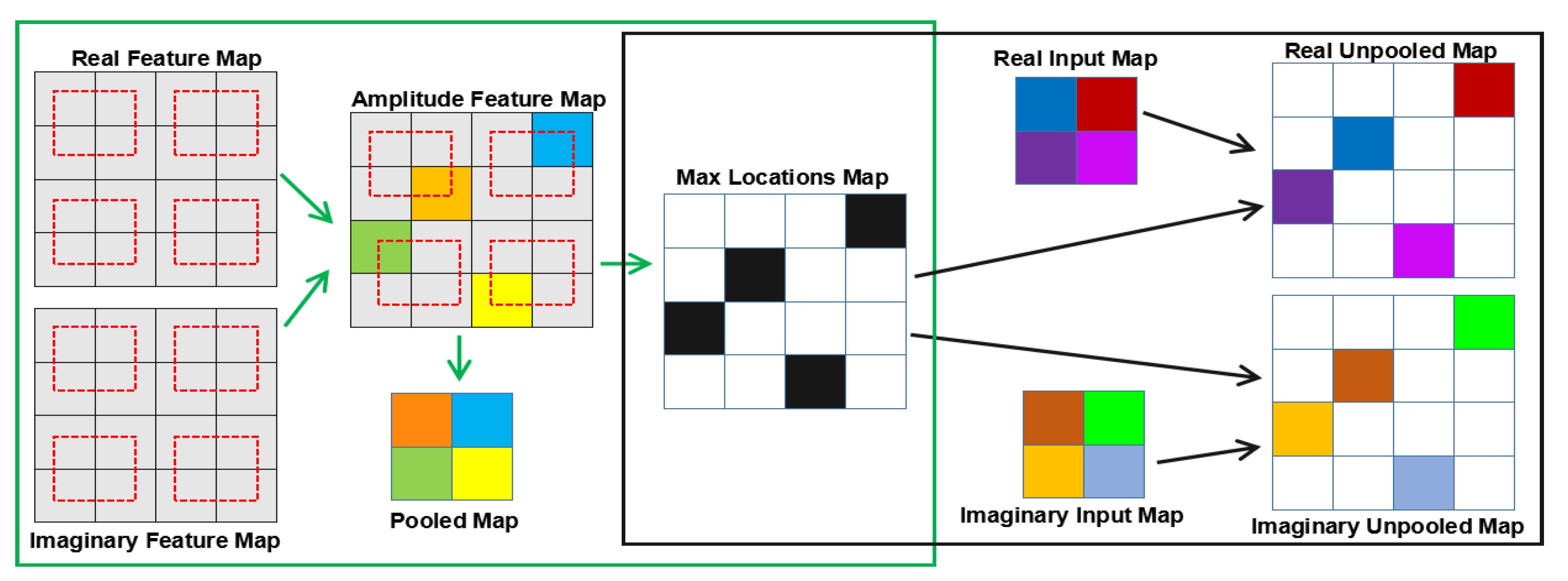
To be more intuitive, Figure 2 illustrates an example of the complex max-unpooling operation. The green and black boxes are simple structures of the complex max-pooling and complex max-unpooling, respectively. As shown in the green box, the amplitude feature map is formed by the real and imaginary feature maps where the red dotted box represents a 2 × 2 pooling window with a stride of 2. In the amplitude feature map, four maximum amplitude values are chosen by corresponding pooling windows which are marked by orange, blue, green, and yellow, respectively. They construct the pooled map. At the same time, locations of those maxima are recorded in a set of switch variables which are visualized by the so-called max locations map. On the other hand, in the black box, the real and imaginary input maps are upsampled by the usage of this max locations map, respectively. Then the real and imaginary unpooled maps are produced. Here, those unpooled maps are sparse wherein white regions have the values of 0. This will ensure that the resolution of the output is higher than the resolution of its input.

In particular, we perform the fully skip connections that can fuse multi-level features to preserve sufficient discriminative information for the classification of complex classes. Finally, the complex output layer with the complex SoftMax function [40] is used to calculate the prediction probability map. Thus, the output of CV-FCN can be formulated as

$$\begin{array}{cc}\hfill O^l& =g\left(Y^{l-1}\right)\hfill \\ \hfill & =g\left(\mathfrak{R}\left(Y^{l-1}\right)\right)+j.g\left(\mathfrak{I}\left(Y^{l-1}\right)\right)\hfill \\ \hfill & =\frac{1}{1+e^{-\mathfrak{R}\left(Y^{l-1}\right)}}+j.\frac{1}{1+e^{-\mathfrak{I}\left(Y^{l-1}\right)}},\hfill \end{array}$$

(13)

where $Y^{l-1}\in {\mathbb{C}}^{H\times W\times K}$ indicates the inputs of the complex output layer and $g(.)$ is the SoftMax function in the real domain. In this layer, output feature maps are the same size as the data patch fed into CV-FCN. This enables pixel-to-pixel training. After the complex downsampling section and the complex upsampling section, the complex forward propagation process of the training phase is completed.

2.4. Average Cross-Entropy Loss Function for Precise CV-FCN Optimization

To promote CV-FCN training more effectively and achieve more precise results, a novel loss function is used as the learning objective to iteratively update CV-FCN parameters $\mathsf{\Theta }$ during the backpropagation. $\mathsf{\Theta }$ includes ${\mathrm{W}}^l$ and $b^l$. Usually, for multi-class classification tasks, the cross-entropy loss function performs well to update parameters. Compared with the quadratic cost function, it can lead to faster convergence and better classification results [48]. Thus, a novel average cross-entropy loss function is employed for predicted CV labels in PolSAR classification tasks, which is based on the definition of the popular cross-entropy loss function. Formally, the average cross-entropy (ACE) loss function is defined as

$$\begin{array}{cc}\hfill J^{ACE}=-\frac{1}{2}·\frac{1}{N}·\sum _{n=1}^N& \left\{\left[\mathfrak{R}\left(R\left[n\right]\right)·ln\left(\mathfrak{R}\left(O\left[n\right]\right)\right)\right.\right.+\left.\left(1-\mathfrak{R}\left(R\left[n\right]\right)\right)·ln\left(1-\mathfrak{R}\left(O\left[n\right]\right)\right)\right]\hfill \\ & +\left[\mathfrak{I}\left(R\left[n\right]\right)·ln\left(\mathfrak{I}\left(O\left[n\right]\right)\right)\right.\left.\left.+\left(1-\mathfrak{I}\left(R\left[n\right]\right)\right)·ln\left(1-\mathfrak{I}\left(O\left[n\right]\right)\right)\right]\right\},\hfill \end{array}$$

(14)

where $O\in {\mathbb{C}}^{H\times W\times K}$ indicates the output data patch in the last complex SoftMax layer and K is the total number of classes. $R\in {\mathbb{C}}^{H\times W\times K}$ denotes the sparse representation of the true label patch $T\in {\mathbb{R}}^{H\times W}$, which is converted by one-hot encoding. Notably, non-zeros positions within $R\in {\mathbb{C}}^{H\times W\times K}$ are $1+1·j$ instead of $1+0·j$. This means that we also take the phase information into account during parameters updating. As a result, the updated CV-FCN can work effectively to provide more precise classification results for PolSAR images.

$\mathsf{\Theta }$ can be updated iteratively by J and learning rate $\eta$ according to

$${\mathrm{W}}_{nm}^l[t+1]={\mathrm{W}}_{nm}^l\left[t\right]-\eta \frac{\partial J\left[t\right]}{\partial {\mathrm{W}}_{nm}^l\left[t\right]},$$

(15)

$$b_n^l[t+1]=b_n^l\left[t\right]-\eta \frac{\partial J\left[t\right]}{\partial b_n^l\left[t\right]}.$$

(16)

To calculate Equation (15) and Equation (16), the key point is to calculate the partial derivatives. Note J is a real-valued loss function, it can be back-propagated through CV-FCN according to the generalized complex chain rule in [36]. Thus, the partial derivatives can be calculated as follows:

$$\begin{array}{cc}\hfill \frac{\partial J}{\partial {\mathrm{W}}_{nm}^l}& =\frac{\partial J}{\partial \mathfrak{R}\left({\mathrm{W}}_{nm}^l\right)}+\frac{\partial J}{\partial \mathfrak{I}\left({\mathrm{W}}_{nm}^l\right)}\hfill \\ \hfill & =\left(\frac{\partial J}{\partial \mathfrak{R}\left({\mathrm{Y}}_n^l\right)}\frac{\partial \mathfrak{R}\left({\mathrm{Y}}_n^l\right)}{\partial \mathfrak{R}\left({\mathrm{W}}_{nm}^l\right)}+\frac{\partial J}{\partial \mathfrak{I}\left({\mathrm{Y}}_n^l\right)}\frac{\partial \mathfrak{I}\left({\mathrm{Y}}_n^l\right)}{\partial \mathfrak{R}\left({\mathrm{W}}_{nm}^l\right)}\right)+j.\left(\frac{\partial J}{\partial \mathfrak{R}\left({\mathrm{Y}}_n^l\right)}\frac{\partial \mathfrak{R}\left({\mathrm{Y}}_n^l\right)}{\partial \mathfrak{I}\left({\mathrm{W}}_{nm}^l\right)}+\frac{\partial J}{\partial \mathfrak{I}\left({\mathrm{Y}}_n^l\right)}\frac{\partial \mathfrak{I}\left({\mathrm{Y}}_n^l\right)}{\partial \mathfrak{I}\left({\mathrm{W}}_{nm}^l\right)}\right),\hfill \end{array}$$

(17)

$$\begin{array}{cc}\hfill \frac{\partial J}{\partial b_n^l}& =\frac{\partial J}{\partial \mathfrak{R}\left(b_n^l\right)}+\frac{\partial J}{\partial \mathfrak{I}\left(b_n^l\right)}\hfill \\ \hfill & =\left(\frac{\partial J}{\partial \mathfrak{R}\left({\mathrm{Y}}_n^l\right)}\frac{\partial \mathfrak{R}\left({\mathrm{Y}}_n^l\right)}{\partial \mathfrak{R}\left(b_n^l\right)}+\frac{\partial J}{\partial \mathfrak{I}\left({\mathrm{Y}}_n^l\right)}\frac{\partial \mathfrak{I}\left({\mathrm{Y}}_n^l\right)}{\partial \mathfrak{R}\left(b_n^l\right)}\right)+j.\left(\frac{\partial J}{\partial \mathfrak{R}\left({\mathrm{Y}}_n^l\right)}\frac{\partial \mathfrak{R}\left({\mathrm{Y}}_n^l\right)}{\partial \mathfrak{I}\left(b_n^l\right)}+\frac{\partial J}{\partial \mathfrak{I}\left({\mathrm{Y}}_n^l\right)}\frac{\partial \mathfrak{I}\left({\mathrm{Y}}_n^l\right)}{\partial \mathfrak{I}\left(b_n^l\right)}\right).\hfill \end{array}$$

(18)

When the value of loss function no longer decreases, the parameter update is suspended, and the training phase is completed. The trained network will then be used to predict the entire PolSAR image in the classification module.

2.5. CV-FCN PolSAR Classification Algorithm

For more intuitive, the proposed CV-FCN PolSAR Classification algorithm is illustrated by Algorithm 1. Specifically, we first construct the entire training set for CV-FCN and employ the new complex-valued weight initialization scheme to initialize the network. Then, we train CV-FCN by alternately updating CV-FCN parameters using the average cross-entropy loss function. Finally, the entire PolSAR image is classified using the trained CV-FCN.

Algorithm 1 CV-FCN classification algorithm for PolSAR imagery

Input: PolSAR dataset $\mathcal{H}\in {\mathbb{C}}^{h\times w\times B}$, ground-truth image $\mathcal{G}\in {\mathbb{R}}^{h\times w}$; learning rate $\eta$, batch size, momentum parameter. 1: Construct the data patches set $\mathcal{I}$ and the label patches set $\mathcal{T}$ using $\mathcal{H}$ and $\mathcal{G}$, respectively; 2: Initialize CV-FCN parameters $\mathsf{\Theta }$ by Section 2.2; 3: Choose the entire training set $D_{train}=\{{\mathcal{I}}_{train},{\mathcal{T}}_{train}\}$ from $\mathcal{I}$ and $\mathcal{T}$; 4: Repeat: 5:    Forward pass the complex downsampling section to obtain multi-level feature maps by Section 2.3.1; 6:    Call the complex upsampling section to recover more spatial information by Section 2.3.2; 7:    Calculate loss function J by Section 2.4; 8:    Update $\mathsf{\Theta }$ by J and $\eta$. 9: Until: meet the termination criterion. 10: Classify the entire PolSAR image by forward passing the trained network to obtain $\mathbf{k}$. 11: End Output: Pixel-wise class labels $\mathbf{k}$.

3. Experimental Results

In this section, experimental datasets description and evaluation metrics are first presented. Then, the input data vector and experimental settings for CV-FCN training are listed. Finally, comparisons with other classification methods on three PolSAR datasets are presented to demonstrate the superiority of the proposed CV-FCN.

3.1. Experimental Datasets Description

We use three benchmark PolSAR datasets for experiments. Details about these datasets are listed as follows.

3.1.1. Flevoland Benchmark Dataset

Figure 3a shows the PauliRGB image of Flevoland Benchmark dataset, which was acquired by NASA/JPL AIRSAR in 1991 and can be downloaded from https://earth.esa.int/web/polsarpro/data-sources/sample-datasets. The size of the image is 1020 × 1024. The ground-truth class labels and the corresponding color codes are shown in Figure 3b,c, respectively. There are 14 classes in the image, including potato, fruit, oats, beet, barley, onions, wheat, beans, peas, maize, flax, rapeseed, grass, and lucerne.

3.1.2. San Francisco Dataset

This AIRSAR full PolSAR image provides good coverage of four targets, including water, vegetation, low-density urban, and high-density urban. The original data has a dimension of 900 × 1024 pixels with a spatial resolution of 10 m, as shown in Figure 4a. The ground-truth class labels and color codes are shown in Figure 4b,c, respectively. This dataset can be downloaded from https://earth.esa.int/web/polsarpro/data-sources/sample-datasets.

3.1.3. Oberpfaffenhofen Dataset

This dataset is an ESAR data of the Oberpfaffenhofen area in Germany, which is provided by the German Aerospace Center. It has a size of 1300 × 1200 pixels, which can be downloaded from https://earth.esa.int/web/polsarpro/data-sources/sample-datasets. The Pauli-RGB image, the ground-truth class labels, and color codes are respectively shown in Figure 5a–c. There are three classes in the image: built-up areas, wood land, and open areas.

3.2. Evaluation Metrics

With the hand-marked ground-truth images, the overall accuracy (OA), average accuracy (AA) and Kappa coefficient ($\kappa$) are used as the evaluation measures for classification performance evaluation. Where OA represents the ratio of the number of correctly labeled pixels divided by the total number of test pixels; AA is defined as the average of individual class accuracy; Kappa, which does not consider the successful classification obtained by chance, gives a good representation of the overall performance of the classifiers. The larger the three criteria values, the better the classification performance.

3.3. Preparing for Classifier Model Training

3.3.1. Complex-Valued Input Vector for CV-FCN

Before training CV-FCN, the CV input vector needs to be determined. CV-FCN works directly on the PolSAR CV data without any data projection from the complex to the real domain. Since the coherency matrix or covariance matrix completely describes the distributed target [1], the PolSAR data is usually presented in these formats. The polarimetric coherency matrix $\mathrm{T}$ is calculated as

$$\mathrm{T}=\frac{1}{L}\sum _{\mathrm{i}=1}^L{\mathrm{u}}_{\mathrm{i}}{\mathrm{u}}_{\mathrm{i}}^{\mathrm{H}}=\left[\begin{array}{ccc}{T}_{11}& T_{12}& T_{13}\\ T_{21}& T_{22}& T_{23}\\ T_{31}& T_{32}& T_{33}\end{array}\right],$$

(19)

where the superscript $\mathrm{H}$ denotes the complex conjugate transpose, L is the number of looks, and ${\mathrm{u}}_{\mathrm{i}}$ denotes the $\mathrm{i}$th scattering vector in the multi-look processing window.

The coherency matrix $\mathrm{T}$ is a Hermitian positive semidefinite matrix, which implies that the main diagonal elements are RV and other CV elements are conjugate symmetric about the main diagonal. Therefore, the six elements of the upper triangular matrix of $\mathrm{T}$ can be used to fully represent the PolSAR data [1]. Therefore, we use these six elements to construct the CV input vector for CV-FCN, which is represented by

$$\left\{T_{11}+0.j,T_{22}+0.j,T_{33}+0.j,T_{12},T_{13},T_{23}\right\}.$$

(20)

Here, imaginary parts of $T_{11},T_{22},T_{33}$ in the CV input feature vector are all expanded with a value of 0. On the other hand, compared with the CV input feature vector with phase information, the RV input feature vector without phase information can be represented by

$$\{T_{11},T_{22},T_{33},\mathfrak{R}\left(T_{12}\right),\mathfrak{R}\left(T_{13}\right),\mathfrak{R}\left(T_{23}\right),\mathfrak{I}\left(T_{12}\right),\mathfrak{I}\left(T_{13}\right),\mathfrak{I}\left(T_{23}\right)\}.$$

(21)

3.3.2. Parameter Settings

Relevant parameter settings are required before CV-FCN training. For the PolSAR image classification, some works of literature have discussed the sampling rate and parameter settings of NNs structures [28,29] in detail. Therefore, we no longer spend time discussing these parameters, and we will select them through experiments.

In this paper, the sliding window operation in [30,49] is used to generate the data patches set from the experimental image and the corresponding label patches set from the ground-truth image. Here, we choose 128 as the default setting of sliding windows size and 25 as the default setting of stride for all experimental datasets, which is a trade between classification performance and computational burden. Additionally, to mitigate overfitting on datasets, the data augmentation strategy [31] was carried out by vertically and horizontally flipping all patches. All these patches are used as input to the proposed CV-FCN, with 90% for training and 10% for validation, respectively. It is worth noting that only the labeled pixels in an individual label patch are considered when modifying network parameters during the training [30].

Moreover, Adam with momentum 0.9 is used to update CV-FCN parameters. The learning rate $\eta$ is 0.0001. The size of the mini-batch is empirically set to 30. The training epoch number is 200 until the model converges. Additionally, dropout regularization is adopted to reduce overfitting. In this paper, all non-deep methods are run on Matlab R2014b, and DL-based methods are implemented in the Keras framework with TensorFlow as the back end. The machine used for experiments is a Lenovo Y720 cube gaming PC with an Intel Core i7-7700 CPU, an Nvidia GeForce GTX 1080 GPU, and 16GB RAM under Ubuntu 18.04 LTS operating system. To make comparisons as fair as possible, all experiments are conducted ten times, and the means and standard deviations of evaluation metrics are reported.

3.4. Comparing Models

We demonstrate the effectiveness of the proposed CV-FCN by comparison with some state-of-art methods including SVM [19], Wishart classifier [4], Markov random field (MRF) [10], MLP [25], CVNN [36], CNN [27], CV-CNN [40], and FCN [30]. In the preceding part, we have already introduced the structure of CV-FCN. The specific settings of comparison methods are briefly described as follows.

• Non-deep methods: The non-deep methods include SVM [19], Wishart classifier [4], and MRF [10]. They all adopt the input feature vector shown in Equation (21). For the SVM-based method, the radial basis function (RBF) kernel is chosen advised by [19]. For MRF, parameters are set according to the original publication [10]. Notably, to compare logically with other spatial methods, we use the post-processing method based on the spatial information [26] to improve the classification performance of the SVM method and the Wishart method.
• RV-FCN: To compare with CV-FCN, we adjust the RV-FCN [30] to have the same structure as CV-FCN. Since the dimension of the input patch for RV-FCN is 9 and the dimension for CV-FCN is 6. For a fair comparison, we adjust the parameter settings of RV-FCN to have the same degree of freedom (DoF) as CV-FCN. We mainly adjust the number of output feature maps in each convolutional layer of RV-FCN, which is about 1.5 times that in CV-FCN.
• RV-MLP/CV-MLP: Referring to [25], we choose a three-layer RV-MLP network, which consists of 128 neurons in the first complex hidden layer and 256 in the second complex hidden layer. The last layer is a SoftMax classifier to predict the probability distribution. For CV-MLP, there are 96 neurons in the first hidden layer and 180 in the second hidden layer. For MLPs, we choose a 32 × 32 neighborhood of each pixel as the patch to networks to consider more contextual information.
• RV-SCNN/CV-SCNN: We use RV-SCNN and CV-SCNN to represent networks in [27,40], respectively. According to RV-SCNN in [27], the architecture of CV-SCNN is adjusted, which contains the input layer, two convolution layers interleaved with two pooling layers, two fully connected layers, and the SoftMax layer.

  Table 2. Detailed configuration of the RV-SCNN and the CV-SCNN. K denotes the total number of classes.

  Network	Module Type	Dimension	Stride	Pad
  RV-SCNN	Convolution	3 × 3 × 9 × 20	1	1
  	ReLU
  	Max-Pooling	2 × 2	2	0
  	Convolution	3 × 3 × 20 × 40	1	1
  	ReLU
  	Max-Pooling	2 × 2	2	0
  	Fully Connection	40 × 2560		1
  	Fully Connection	2560 × K		1
  	SoftMax
  CV-SCNN	Complex Convolution	3 × 3 × 6 × 12	1	1
  	$\mathbb{C}$ReLU
  	Complex Max-Pooling	2 × 2	2	0
  	Complex Convolution	3 × 3 × 12 × 24	1	1
  	$\mathbb{C}$ReLU
  	Complex Max-Pooling	2 × 2	2	0
  	Complex Fully Connection	24 × 1536		1
  	Complex Fully Connection	1536 × K		1
  	Complex SoftMax

  reports the detailed configuration of RV-SCNN and CV-SCNN. For SCNNs, a 32 × 32 neighborhood of each pixel is employed as the patch for training.
• RV-DCNN/CV-DCNN: The downsampling section of FCN is transformed from a CNN structure. Therefore, for a fair comparison between FCN and CNN, we construct a new CNN structure represented by DCNN based on the CV-FCN structure.

  Table 3. Detailed configuration of the RV-DCNN and the CV-DCNN. K denotes the total number of classes. The ReLU layers in RV-DCNN, complex BN layers and $\mathbb{C}$ReLU layers in CV-DCNN are omitted for brevity.

  Network	Module Type	Dimension	Stride	Pad
  RV-DCNN	Convolution	3 × 3 × 9 × 18	1	1
  	Max-Pooling	2 × 2	2	0
  	Convolution	3 × 3 × 18 × 36	1	1
  	Max-Pooling	2 × 2	2	0
  	Convolution	3 × 3 × 36 × 72	1	1
  	Max-Pooling	2 × 2	2	0
  	Convolution	3 × 3 × 72 × 144	1	1
  	Max-Pooling	2 × 2	2	0
  	Convolution	3 × 3 × 144 × 288	1	1
  	Max-Pooling	2 × 2	2	0
  	Fully Connection	288 × 288		1
  	Fully Connection	288 × K		1
  	SoftMax
  CV-DCNN	Complex Convolution	3 × 3 × 6 × 12	1	1
  	Complex Max-Pooling	2 × 2	2	0
  	Complex Convolution	3 × 3 × 12 × 24	1	1
  	Complex Max-Pooling	2 × 2	2	0
  	Complex Convolution	3 × 3 × 24 × 48	1	1
  	Complex Max-Pooling	2 × 2	2	0
  	Complex Convolution	3 × 3 × 48 × 96	1	1
  	Complex Max-Pooling	2 × 2	2	0
  	Complex Convolution	3 × 3 × 96 × 192	1	1
  	Complex Max-Pooling	2 × 2	2	0
  	Complex Fully Connection	192 × 192		1
  	Complex Fully Connection	192 × K		1
  	Complex SoftMax

  reports the detailed configuration of RV-DCNN and CV-DCNN. Compared with CNNs in [40], DCNNs contain more convolutional layers. For DCNNs, we have the same operation as SCNNs to generate patches for training.

3.5. Classification Performance Evaluation

To evaluate the effectiveness of CV-FCN, comparisons with the above models on three PolSAR datasets are presented as follows.

3.5.1. Flevoland Benchmark Dataset Result

For this dataset, we randomly choose 5% of available labeled samples per class for training. The classification maps obtained from all methods are shown in Figure 6, and the accuracies are reported in

Table 4. Individual class, overall, average accuracies (%) and Kappa coefficient of all competing methods on the Flevoland Benchmark PolSAR image.

Class	SVM	Wishart	MRF	RV-MLP	RV-SCNN	RV-DCNN	RV-FCN	CV-MLP	CV-SCNN	CV-DCNN	CV-FCN
1	98.11 ± 0.12	92.95 ± 0.40	99.26 ± 0.16	99.01 ± 0.27	99.86 ± 0.08	99.90 ± 0.08	99.89 ± 0.10	99.14 ± 0.17	99.63 ± 0.09	99.69 ± 0.10	99.98 ± 0.05
2	98.13 ± 0.20	93.70 ± 0.54	96.78 ± 0.40	99.98 ± 0.16	98.87 ± 0.68	98.19 ± 1.10	99.05 ± 1.67	88.54 ± 1.96	97.37 ± 1.16	96.53 ± 1.21	99.97 ± 0.09
3	94.53 ± 0.25	93.64 ± 0.22	96.63 ± 0.19	83.14 ± 2.62	55.42 ± 1.85	99.97 ± 0.09	66.94 ± 1.47	95.34 ± 0.44	100 ± 0	100 ± 0	77.57 ± 0.49
4	80.60 ± 1.37	76.13 ± 1.20	82.25 ± 1.43	76.91 ± 0.96	84.87 ± 1.47	83.25 ± 1.29	99.28 ± 0.92	80.82 ± 1.71	85.52 ± 1.73	90.42 ± 2.34	99.97 ± 0.02
5	89.59 ± 0.69	85.28 ± 0.96	93.47 ± 0.93	99.91 ± 0.05	100 ± 0	99.99 ± 0.02	99.67 ± 0.54	99.65 ± 0.28	99.76 ± 0.53	100 ± 0	100 ± 0
6	38.90 ± 1.86	35.71 ± 1.56	32.68 ± 2.24	56.81 ± 1.21	65.36 ± 2.94	89.08 ± 1.58	69.89 ± 0.88	50.80 ± 2.27	83.50 ± 1.49	89.13 ± 1.92	99.24 ± 0.14
7	93.90 ± 0.43	95.27 ± 0.45	97.27 ± 0.30	99.92 ± 0.07	99.97 ± 0.03	99.99 ± 0.03	99.96 ± 0.06	99.86 ± 0.10	99.99 ± 0.01	99.97 ± 0.01	100 ± 0
8	97.54 ± 0.45	92.30 ± 0.51	99.54 ± 0.37	81.33 ± 0.48	82.57 ± 1.91	88.69 ± 1.72	90.51 ± 1.68	71.16 ± 1.02	91.65 ± 2.40	97.79 ± 1.80	98.79 ± 1.11
9	99.86 ± 0.01	99.91 ± 0.02	99.95 ± 0.04	100 ± 0	99.96 ± 0.07	100 ± 0	99.82 ± 0.40	100 ± 0	100 ± 0	100 ± 0	99.90 ± 0.13
10	76.19 ± 1.83	72.47 ± 1.54	14.19 ± 2.75	98.91 ± 0.28	93.23 ± 1.06	87.74 ± 1.80	91.00 ± 0.86	99.53 ± 0.17	90.12 ± 1.29	98.15 ± 1.04	98.85 ± 1.21
11	99.51 ± 0.05	97.69 ± 0.29	99.51 ± 0.04	61.78 ± 1.68	56.41 ± 2.59	69.04 ± 2.16	99.79 ± 0.54	87.77 ± 1.13	64.96 ± 2.06	96.65 ± 0.26	99.97 ± 0.03
12	95.46 ± 0.48	76.88 ± 0.90	94.76 ± 0.74	100 ± 0	100 ± 0	100 ± 0	99.94 ± 0.07	100 ± 0	99.98 ± 0.03	100 ± 0	99.99 ± 0.01
13	73.71 ± 0.84	69.31 ± 1.27	74.22 ± 0.92	88.13 ± 0.78	98.54 ± 0.71	99.12 ± 0.86	93.53 ± 1.31	83.11 ± 1.21	98.35 ± 0.67	100 ± 0	99.87 ± 0.19
14	88.63 ± 0.38	88.76 ± 0.40	89.19 ± 0.52	98.95 ± 0.38	99.93 ± 0.09	100 ± 0	99.36 ± 0.26	98.17 ± 0.72	99.99 ± 0.02	100 ± 0	99.97 ± 0.08
OA	91.72 ± 0.17	85.68 ± 0.24	92.58 ± 0.21	95.34 ± 0.51	96.09 ± 0.30	97.18 ± 1.00	98.63 ± 0.96	96.21 ± 0.53	97.06 ± 0.25	98.75 ± 0.49	99.72 ± 0.42
AA	87.47 ± 0.51	83.57 ± 0.34	83.55 ± 1.15	88.91 ± 0.21	88.21 ± 0.65	93.92 ± 1.02	93.47 ± 0.51	90.35 ± 1.19	93.63 ± 0.57	97.74 ± 0.67	98.14 ± 0.89
kappa	0.9033 ± 0.0021	0.8336 ± 0.0027	0.9131 ± 0.0024	0.9450 ± 0.0061	0.9538 ± 0.0035	0.9668 ± 0.0118	0.9837 ± 0.0112	0.9554 ± 0.0062	0.9654 ± 0.0030	0.9853 ± 0.0049	0.9967 ± 0.0049

.

As shown in Figure 6b–d, non-deep methods perform badly in recognizing different categories. Although non-deep methods can clearly classify wheat class and flax class, they cannot recognize onions class and grass class well. Figure 6e–l demonstrate the classification results for all DL-based methods, where Figure 6e–h are the results of different RV-NNs and Figure 6i–l give the results of different CV-NNs. As shown, all DL-based methods outperform non-deep methods, which indicates that learning features have stronger discriminative ability than traditional features.

When comparing RV-NNs, it can be seen that RV-FCN performs best for the classification of flax class [marked by white ovals in Figure 6e–h]. In addition, among CV-NNs, CV-FCN has the highest classification accuracy on the beet class [marked by yellow ovals in Figure 6i–l], and the whole class label map of CV-FCN is much clearer than others. The above two results indicate that proposed FCN architecture is advantageous for PolSAR classification compared to other network structures, especially CNNs.

Moreover, comparing RV-NNs and CV-NNs directly, we can observe that CV-NNs have better performance than their RV counterparts. For example, Figure 6h,l are classification results from RV-FCN and CV-FCN, respectively. The confusion between oats class and beet class is severe in Figure 6h but does not appear in Figure 6l [marked by sky-blue rectangles]. This confirms the effectiveness of complex-valued features with the phase information for the classification of PolSAR imagery. From the overall effects depicted in Figure 6, the classification map of CV-FCN is noticeably closer to the ground-truth map.

The evaluation indices of all methods are listed in Table 4. As shown in Table 4, all DL-based methods achieve OA exceeding 95%. All CV-NNs methods achieve better performance than their RV counterparts in terms of all evaluation metrics. In particular, the largest part of changes in metrics is AA values. Furthermore, CV-FCN outperforms other compared methods in terms of three quantitative criteria. Although compared with CV-DCNN, CV-FCN attains only 0.97% improvement in terms of OA, all classes besides oats show comparable or higher accuracy which is consistent with the results shown in Figure 6. In summary, from Figure 6 and Table 4, for the Flevoland Benchmark dataset, CV-FCN achieves the best performance compared with other methods and has the powerful ability to distinguish different terrain categories.

3.5.2. San Francisco Dataset Result

For the San Francisco dataset, we randomly choose 1% labeled pixels per class for training, and the remaining for testing. The classification results obtained from all methods are shown in Figure 7, and

Table 5. Individual class, overall, average accuracies (%) and Kappa coefficient of all competing methods on the San Francisco PolSAR image.

Class	SVM	Wishart	MRF	RV-MLP	RV-SCNN	RV-DCNN	RV-FCN	CV-MLP	CV-SCNN	CV-DCNN	CV-FCN
1	100 ± 0	96.43 ± 0.19	99.37 ± 0.01	99.05 ± 0.20	97.78 ± 1.42	93.35 ± 1.33	99.62 ± 0.35	99.12 ± 0.18	99.68 ± 0.07	97.59 ± 1.39	99.98 ± 0.03
2	89.08 ± 0.31	85.79 ± 1.00	89.09 ± 0.32	91.65 ± 0.99	84.77 ± 1.38	97.10 ± 1.10	98.91 ± 0.61	93.28 ± 0.87	89.68 ± 1.87	98.69 ± 0.44	99.38 ± 0.35
3	80.17 ± 0.72	63.94 ± 1.66	82.85 ± 0.59	90.51 ± 1.74	96.88 ± 1.43	95.16 ± 0.77	96.68 ± 1.30	92.34 ± 1.26	96.50 ± 0.84	95.75 ± 0.57	99.54 ± 0.40
4	81.65 ± 1.10	68.57 ± 0.84	82.16 ± 0.77	96.91 ± 0.27	98.09 ± 0.56	99.81 ± 0.15	98.79 ± 0.68	96.65 ± 0.42	97.62 ± 1.43	99.45 ± 0.30	99.72 ± 0.16
OA	90.04 ± 0.08	82.10 ± 0.39	90.53 ± 0.08	94.96 ± 0.37	94.23 ± 1.50	95.74 ± 1.01	98.61 ± 0.55	95.77 ± 0.64	96.26 ± 0.68	97.74 ± 0.36	99.69 ± 0.13
AA	87.73 ± 0.09	78.68 ± 0.44	88.37 ± 0.10	94.53 ± 0.36	93.96 ± 1.69	96.36 ± 1.21	98.49 ± 0.56	95.35 ± 0.62	95.87 ± 0.70	97.87 ± 0.27	99.65 ± 0.13
kappa	0.8615 ± 0.0012	0.7531 ± 0.0053	0.8683 ± 0.0008	0.9303 ± 0.0050	0.9203 ± 0.0206	0.9416 ± 0.0269	0.9807 ± 0.0077	0.9415 ± 0.0088	0.9483 ± 0.0093	0.9687 ± 0.0050	0.9957 ± 0.0018

reports the evaluation metrics of them.

Figure 7b–d demonstrate the classification results using non-deep classifiers. It can be viewed that vegetation, low-density urban and high-density urban are severely mixed, and there are many misclassified areas. We conjecture that due to the limited discriminative features, it is difficult for non-deep methods to distinguish complex backscatters, especially for vegetation and urban areas. Figure 7e–l show the classification results of DL-based methods. From Figure 7e–h, it is worth noting that RV-FCN outperforms than the other three methods, and the boundaries between categories are much clearer. In addition, from Figure 7i–l, CV-FCN yields the optimal visual effect compared with other CV-NNs. All the above analyses about NNs demonstrate the effectiveness of the proposed FCN structure, which can capture more discriminative features and effectively incorporate more spatial information. Furthermore, from Figure 7, CV-FCN achieves the best performance, which illustrates that both the FCN structure and the phase information have contributions to improve classification accuracies.

As Table 5 shows, CV-FCN achieves the highest classification accuracy. The OA value of CV-FCN is about 3% and 4% higher than CV-DCNN and CV-SCNN, respectively, which indicates the superiority of the proposed FCN structure for PolSAR classification. In addition, the results of CV-FCN are better than RV-FCN. This confirms that the phase information plays an important role in the improvement of classification accuracy. Furthermore, CV-FCN yields the highest accuracies in all evaluation metrics, which is coincident with results in Figure 7.

3.5.3. Oberpfaffenhofen Dataset Result

For the Oberpfaffenhofen dataset, we choose 1% of pixels with ground-truth class labels for training. Figure 8 shows the visual classification results. The overall evaluation indices are given in

Table 6. Individual class, overall, average accuracies (%) and Kappa coefficient of all competing methods on the Oberfaffenhofen PolSAR image.

Method	SVM	Wishart	MRF	RV-MLP	RV-SCNN	RV-DCNN	RV-FCN	CV-MLP	CV-SCNN	CV-DCNN	CV-FCN
OA	83.05 ± 0.07	82.00 ± 0.11	83.70 ± 0.04	89.36 ± 1.30	93.35 ± 0.33	94.75 ± 0.88	95.51 ± 0.50	90.02 ± 0.56	93.52 ± 0.12	95.76 ± 0.57	97.26 ± 0.33
AA	76.99 ± 0.15	75.88 ± 0.26	77.83 ± 0.12	86.27 ± 0.56	94.16 ± 0.15	93.42 ± 1.33	94.38 ± 0.72	86.39 ± 0.71	93.46 ± 0.35	94.87 ± 0.73	96.38 ± 0.43
kappa	0.7045 ± 0.0014	0.6862 ± 0.0021	0.7156 ± 0.0009	0.8186 ± 0.0082	0.8889 ± 0.0051	0.9097 ± 0.0156	0.9227 ± 0.0086	0.8279 ± 0.0090	0.8909 ± 0.0023	0.9274 ± 0.0098	0.9531 ± 0.0056

, and Figure 9 demonstrates the classification accuracies of every class obtained from different methods.

In Table 6, CV-FCN achieves the best performance in terms of all metrics. The accuracies of non-deep methods are poor which are all below 85% in terms of OA. This might be a result of limited labeled pixels as prior information and little discriminative features. It can also be seen that CV-NNs have better performance than their RV counterparts. However, this superiority is not prominent. In terms of OA, CV-MLP, CV-SCNN, CV-DCNN, and CV-FCN are only 0.66%, 0.17%, 1.01%, and 1.75% higher than RV-MLP, RV-SCNN, RV-DCNN, and RV-FCN, respectively.

Figure 8e–l show classification results of RV-NNs and CV-NNs, respectively. As shown in Figure 8e–h, the classification result using RV-FCN is much clear than the other three, especially in the purple boxes which are noticeably closer to the ground-truth map. This situation also occurs in the comparison among CV-NNs. Comparing all results shown in Figure 8, for this dataset, the classification map of CV-FCN is the best close to the ground-truth map.

As shown in Figure 9, non-deep methods have poor abilities to distinguish built-up areas and wood land. That can also be observed in Figure 8b–d where the misclassification in whole images is severe and all classification maps have many isolated pixels. However, the accuracies of wood land and open areas using DCNNs and FCNs are all over 95%, which illustrates the discriminative feature learning ability of deep networks. In addition, CV-FCN is advantageous in terms of accuracies for all categories relative to other methods, which demonstrates its effectiveness in extracting more discriminative features. Overall, the above analyses precisely illustrate that CV-FCN can exhibit better contextual consistency and extract more discriminative features from PolSAR imagery.

As demonstrated in the above comparisons, the classification performance of CV-FCN exceeds other methods on all PolSAR datasets. On the one hand, CV-FCN effectively improves the classification accuracy compared to its RV counterpart (i.e., RV-FCN). Meanwhile, this conclusion is also established in other network structures, which confirms the validity of complex-valued features containing the phase information. On the other hand, compared with CNN structures, CV-FCN can perform more coherent labeling and exhibit better robustness to the speckle noise, while resulting in smooth classification with precise location. This demonstrates the effectiveness of CV-FCN architecture in considering more spatial information and extracting more discriminative features for PolSAR image classification.

4. Discussion

To evaluate the performance of some aspects of the CV-FCN model, we conduct two ablation experiments and two comparison experiments as follows. Notably, the most perspective of the proposed CV-FCN is the complex-valued upsampling scheme, where the fully skip connections and the max locations maps are the two critical strategies. Therefore, two ablation experiments are designed for comparison and evaluation. Specifically, the impact of fully skip connections in the CV-FCN structure is investigated first. Then, the effect of max locations maps on classification performance is evaluated on all datasets. Additionally, a comparison experiment about the new complex-valued weight initialization scheme is conducted. Finally, the effectiveness of different loss functions on precise classification is compared. The two ablation experiments are all conducted on all three datasets. Moreover, the third experiment and the fourth experiment are conducted on the Flevoland Benchmark dataset and the Oberpfaffenhofen dataset, respectively.

4.1. Ablation Experiment 1—Impact of Fully Skip Connections

The fully skip connection is an important part of CV-FCN because it enables the network to enhance more feature details. The core idea is to superimpose feature maps of different levels to improve the final classification effect. Here, to evaluate the effectiveness of fully skip connections on classification accuracy, we construct the CV-FCN structure without skip connections. We use NS_CV-FCN to represent this CV-FCN network.

Table 7. Overall, average accuracies (%) and Kappa coefficient of the NS_CV-FCN method and the CV-FCN method.

Dataset	Methods	OA	AA	Kappa
Flevoland	NS_CV-FCN	98.73	94.97	0.9851
	CV-FCN	99.72	98.14	0.9967
SanFrancisco	NS_CV-FCN	98.37	98.12	0.9774
	CV-FCN	99.69	99.65	0.9957
Oberpfaffenhofen	NS_CV-FCN	93.36	90.51	0.8831
	CV-FCN	97.26	96.38	0.9531

contains the evaluation indices for classification.

As illustrated in Table 7, CV-FCN outperforms NS_CV-FCN, which reveals that fully skip connections are useful for improving classification accuracy. Compared with NS_CV-FCN, the proposed CV-FCN increases the accuracy by 0.99% of OA, 3.17% of AA, and 0.0116 of the Kappa coefficient, respectively, on the Flevoland dataset. Moreover, on the SanFrancisco dataset, CV-FCN can achieve the accuracy increments by 1.32% of OA, 1.53% of AA, and 0.0183 of Kappa, respectively. In particular, on the Oberpfaffenhofen dataset, CV-FCN increases the accuracy significantly by 3.9% of OA, 5.87% of AA, and 0.07 of Kappa, respectively. This superiority can be attributed to the fact that fully skip connections fuse features of different levels to preserve more discriminative information for PolSAR image classification.

4.2. Ablation Experiment 2—Impact of Max Locations Maps

The most prominent trait in the complex upsampling section is that the max locations maps are used to perform nonlinear upsampling of the feature maps, which are beneficial for more precise reconstruction output. To examine the effect of max locations maps, we construct a CV-FCN structure wherein complex upsampling layers upsample feature maps without the guidance of max locations maps. We call this network NL_CV-FCN. The experimental results on all datasets are shown in

Table 8. Overall, average accuracies (%) and Kappa coefficient of the NL_CV-FCN method and the CV-FCN method.

Dataset	Methods	OA	AA	Kappa
Flevoland	NL_CV-FCN	99.29	96.41	0.9915
	CV-FCN	99.72	98.14	0.9967
SanFrancisco	NL_CV-FCN	98.97	98.84	0.9857
	CV-FCN	99.69	99.65	0.9957
Oberpfaffenhofen	NL_CV-FCN	95.80	94.31	0.9273
	CV-FCN	97.26	96.38	0.9531

.

As illustrated in Table 8, CV-FCN outperforms NL_CV-FCN on all three datasets. Specifically, CV-FCN is able to achieve the accuracy increments by 0.43% of OA, 1.73% of AA, and 0.0052 of Kappa, respectively, on the Flevoland dataset; by 0.72% of OA, 0.81% of AA, and 0.001 of Kappa, respectively, on the SanFrancisco dataset; by 1.46% of OA, 2.07% of AA, and 0.0258 of Kappa, respectively, on the Oberpfaffenhofen dataset. These results suggest that the max locations maps benefit the classification accuracy since they have the capacity to retrieve sufficient spatial information.

4.3. Comparison Experiment 1—Complex-Valued Weight Initialization

To evaluate the impact of complex-valued weight initialization, which is critical for CV-FCN learning, we conduct a comparison experiment on the Flevoland Benchmark dataset. We only use the complex-valued weight initialization in [40] as the old CV initialization scheme for comparison. The old CV initialization scheme is to initialize the real and imaginary parts of a CV weight separately with a uniform distribution [40]. Figure 10 illustrates the difference in the validation curves of one presentative experiment, where the proposed weight initialization and the compared weight initialization are denoted by CWI-1 and CWI-2, respectively. Furthermore, we also report the evaluation indices of two initialization schemes as a function of epoch. Specifically, we first train CV-FCN for 10 epochs and then update classification results every 10 epochs.

Table 9. Overall, average accuracies (%) and Kappa coefficient of different complex weight initialization methods on the Flevoland Benchmark PolSAR image.

Epochs		10	20	30	40	50	60	70	80	90	100	110	120	130	140
CWI-1	OA	68.51	84.58	89.05	94.99	96.08	97.56	97.78	98.54	99.03	99.12	98.85	99.25	98.40	97.60
	AA	28.55	48.55	62.30	75.13	79.90	88.89	89.31	96.34	96.56	96.66	95.82	98.02	96.30	95.14
	Kappa	0.6163	0.8174	0.8709	0.9410	0.9539	0.9713	0.9738	0.9828	0.9885	0.9897	0.9865	0.9912	0.9812	0.9717
CWI-2	OA	91.78	94.89	97.79	99.09	98.93	99.36	98.07	98.81	98.03	98.77	98.79	97.70	95.17	94.11
	AA	67.31	75.51	90.08	96.59	96.99	98.08	95.06	96.26	95.64	97.50	97.13	94.11	94.95	73.15
	Kappa	0.9029	0.9398	0.9740	0.9893	0.9874	0.9925	0.9773	0.9865	0.9768	0.9855	0.9857	0.9729	0.9434	0.9305

contains a comparison of the results.

As shown in Figure 10, both old initialization and proposed initialization lead to convergence, but proposed initialization trains CV-FCN faster and reaches the optimal value earlier. As illustrated in Table 9, the proposed initialization achieves the best results when the training epoch is set as around 60, while the old initialization achieves is around 120. These results validate that the proposed initialization not only facilitates faster learning but also improves the classification performance of CV-FCN. It may be attributed to the ability of proposed initialization to reduce risks of vanishing or exploding gradients, which has great significance for deep networks training. Additionally, these phenomena partially illustrate that the proposed initialization scheme is suitable for CV-FCN to achieve a given PolSAR image classification task.

4.4. Comparison Experiment 2—Loss Function

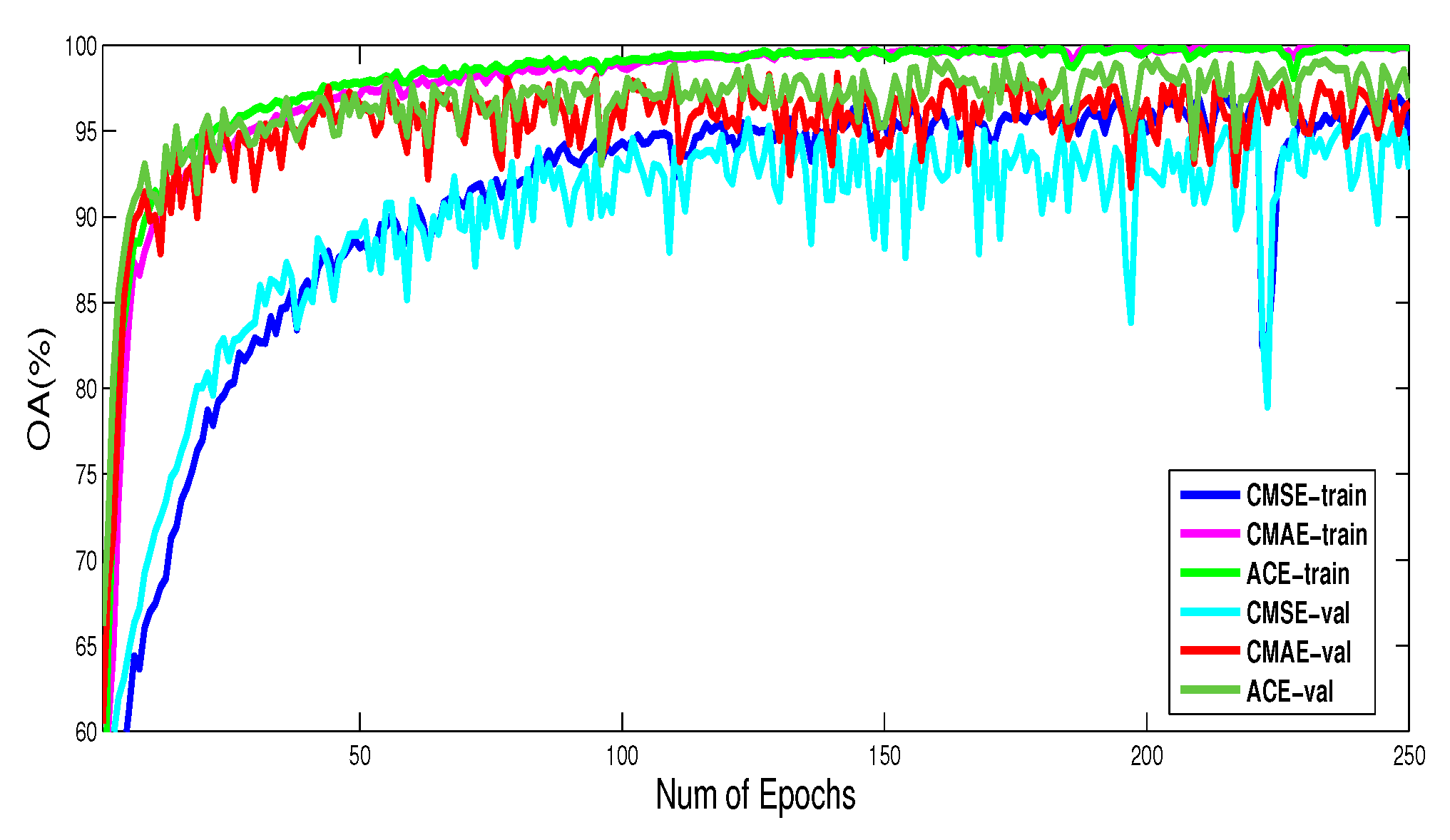
We carry out a comparison experiment on the Oberpfaffenhofen dataset to evaluate the effectiveness of the average cross-entropy loss function (ACE). The complex-valued mean square error (MSE) [40] and the complex-valued mean absolute error (MAE) are loss functions for comparison, which will be respectively denoted by CMSE and CMAE. The CMSE and the CMAE can be respectively expressed as

$$J^{CMSE}=\frac{1}{2N}·\sum _{n=1}^N\left[{(\mathfrak{R}\left(R\left[n\right]\right)-\mathfrak{R}\left(O\left[n\right]\right))}^2+{(\mathfrak{I}\left(R\left[n\right]\right)-\mathfrak{I}\left(O\left[n\right]\right))}^2\right],$$

(22)

$$J^{CMAE}=\frac{1}{N}·\sum _{n=1}^N\left[\right|\mathfrak{R}\left(R\left[n\right]\right)-\mathfrak{R}\left(O\left[n\right]\right)|+|\mathfrak{I}\left(R\left[n\right]\right)-\mathfrak{I}\left(O\left[n\right]\right)\left|\right].$$

(23)

The overall accuracy curves of training and validation using different loss functions are illustrated in Figure 11. Moreover, the typical classification maps using different loss functions are shown in Figure 12.

As seen from Figure 11, CV-FCN using ACE and CMAE can converge faster than CMSE. The training and validation curves using ACE and CMAE remain relatively stable after 120 epochs, while curves using CMSE still do not achieve similar stability until 250 epochs. Additionally, the best accuracy of the proposed loss function is higher than CMAE when validation. As shown in Figure 12, the classification map using CMSE is smoother than CMAE and ACE. This finding is potentially explained that CV-FCN using CMSE can mitigate the effects of the speckle noise. However, boundary delineations between different categories are ambiguous due to being too smooth. Although the classification map using CMAE contains clear structural information, it has more misclassification points due to the speckle noise. Notably, CV-FCN using the proposed ACE can achieve correct boundary localization as well as show better robustness to speckle noise. Thus, these above phenomena can partially establish the effectiveness of the proposed loss function.

5. Conclusions

In this paper, a novel complex-valued (CV) pixel-level model called CV-FCN has been proposed for PolSAR image classification, which obtains better classification performance than non-deep methods and other DL-based methods. This model integrates the feature extraction module and the classification module in a unified framework. For learning meaningful features faster, a new complex-valued weight initialization scheme is proposed to initialize CV-FCN. It greatly facilitates faster learning for this network and is beneficial to improve CV-FCN performance. Then, different-level and robust CV features that retain more discriminative information are extracted via CV-FCN. In particular, a new complex upsampling scheme in CV-FCN is proposed to output CV predicted labeling. It also recovers rich spatial information with max locations maps to alleviate the problem of speckle noise. Furthermore, a novel average cross-entropy loss function is presented for more precise CV-FCN optimization. The proposed CV-FCN model can directly use the PolSAR CV data to enable pixel-to-pixel classification results without any data projection. Moreover, it automatically learns higher-level feature representations and fuses multi-level features for accurate category identification. Experimental results on real benchmark PolSAR images show that CV-FCN achieves comparable or better results than the comparing models.

In the future, this work may be continued with the following ideas: (1) Although some experiments have demonstrated the effectiveness of the new complex-valued weight initialization scheme, it still needs strong cues to prove the superiority and some visualization to observe the difference; (2) With the limitation of available PolSAR datasets and high-quality training datasets, training deeper complex-valued networks devoted to PolSAR classification is very challenging, often yielding the risk of overfitting and model collapse. Moreover, data augmentation strategies for natural images are generally not suited for PolSAR images to enlarge training datasets because of the difference in imaging mechanisms. So, it appears that an available data augmentation strategy is urgently necessary to tackle the above issues.

References

- Lee, J.S.; Pottier, E. Polarimetric Radar Imaging: From Basic to Application; CRC Press: Boca Raton, FL, USA, 2011. [Google Scholar]
- Hänsch, R.; Hellwich, O. Skipping the real world: Classification of PolSAR images without explicit feature extraction. ISPRS J. Photogramm. Remote Sens. 2018, 140, 122–132. [Google Scholar] [CrossRef]
- Lee, J.S.; Grunes, M.R.; Kwok, R. Classification of multi-look polarimetric SAR imagery based on the complex Wishart distribution. Int. J. Remote Sens. 1994, 15, 2299–2311. [Google Scholar] [CrossRef]
- Lee, J.S.; Grunes, M.R.; Pottier, E.; Ferro-Famil, L. Unsupervised terrain classification preserving polarimetric scattering characteristics. IEEE Trans. Geosci. Remote Sens. 2004, 42, 722–731. [Google Scholar]
- Dabboor, M.; Collins, M.; Karathanassi, V.; Braun, A. An unsupervised classification approach for polarimetric SAR data based on the Chernoff distance for the complex Wishart distribution. IEEE Trans. Geosci. Remote Sens. 2013, 51, 4200–4213. [Google Scholar] [CrossRef]
- Cloude, S.R.; Pottier, E. A review of target decomposition theorems in radar polarimetry. IEEE Trans. Geosci. Remote Sens. 1996, 34, 498–518. [Google Scholar] [CrossRef]
- Clound, S.R.; Pottier, E. An entropy based classification scheme for land applications of polarimetric SAR. IEEE Trans. Geosci. Remote Sens. 1997, 35, 68–78. [Google Scholar]
- An, W.; Cui, Y.; Yang, J. Three-Component Model-Based Decomposition for Polarimetric SAR Data. IEEE Trans. Geosci. Remote Sens. 2010, 48, 2732–2739. [Google Scholar]
- Arii, M.; van Zyl, J.J.; Kim, Y. Adaptive model-based decomposition of polarimetric SAR covariance matrices. IEEE Trans. Geosci. Remote Sens. 2011, 49, 1104–1113. [Google Scholar] [CrossRef]
- Wu, Y.; Ji, K.; Yu, W.; Su, Y. Region-based classification of polarimetric SAR images using Wishart MRF. IEEE Geosci. Remote Sens. Lett. 2008, 5, 668–672. [Google Scholar] [CrossRef]
- Liu, G.; Li, M.; Wu, Y.; Jia, L.; Liu, H.; Zhang, P. PolSAR image classification based on Wishart TMF with specific auxiliary field. IEEE Geosci. Remote Sens. Lett. 2014, 11, 1230–1234. [Google Scholar]
- Song, W.; Li, M.; Zhang, P.; Wu, Y.; Tan, X.; An, L. Mixture WGΓ-MRF model for PolSAR image classification. IEEE Trans. Geosci. Remote Sens. 2018, 56, 905–920. [Google Scholar] [CrossRef]
- Chen, C.; Chen, K.; Lee, J. The use of fully polarimetric information for the fuzzy neural classification of SAR images. IEEE Trans. Geosci. Remote Sens. 2003, 41, 2089–2100. [Google Scholar] [CrossRef]
- Kandaswamy, U.; Adjeroh, D.; Lee, M. Efficient texture analysis of SAR imagery. IEEE Trans. Geosci. Remote Sens. 2005, 43, 2075–2083. [Google Scholar] [CrossRef]
- He, C.; Li, S.; Liao, Z.; Liao, M. Texture Classification of PolSAR Data Based on Sparse Coding of Wavelet Polarization Textons. IEEE Trans. Geosci. Remote Sens. 2013, 51, 4576–4590. [Google Scholar] [CrossRef]
- Kahaki, S.M.M.; Nordin, M.J.; Ashtari, A.H. Contour-Based Corner Detection and Classification by Using Mean Projection Transform. Sensors 2014, 14, 4126–4143. [Google Scholar] [CrossRef]
- Uhlmann, S.; Kiranyaz, S. Integrating color features in polarimetric SAR image classification. IEEE Trans. Geosci. Remote Sens. 2014, 52, 2197–2216. [Google Scholar] [CrossRef]
- Zhang, Q.; Wei, X.; Xiang, D.; Sun, M. Supervised PolSAR Image Classification with Multiple Features and Locally Linear Embedding. Sensors 2018, 18, 3054. [Google Scholar] [CrossRef]
- Lardeux, C.; Frison, P.L.; Tison, C.C.; Souyris, J.C.; Stoll, B.; Fruneau, B.; Rudant, J.P. Support vector machine for multifrequency SAR polarimetric data classification. IEEE Trans. Geosci. Remote Sens. 2009, 47, 4143–4152. [Google Scholar] [CrossRef]
- Zhu, X.X.; Tuia, D.; Mou, L.; Xia, G.-S.; Zhang, L.; Xu, F.; Fraundorfer, F. Deep Learning in Remote Sensing: A Comprehensive Review and List of Resources. IEEE Trans. Geosci. Remote Sens. 2017, 5, 8–36. [Google Scholar] [CrossRef]
- Ghosh, A.; Subudhi, B.N.; Bruzzone, L. Integration of Gibbs Markov random field and Hopfield-type neural networks for unsupervised change detection in remotely sensed multitemporal images. IEEE Trans. Image Process. 2013, 22, 3087–3096. [Google Scholar] [CrossRef]
- Geng, J.; Wang, H.; Fan, J.; Ma, X. Deep Supervised and Contractive Neural Network for SAR Image Classification. IEEE Trans. Geosci. Remote Sens. 2017, 55, 2442–2459. [Google Scholar] [CrossRef]
- Kahaki, S.M.M.; Nordin, M.J.; Ahmad, N.S.; Arzoky, M.; Ismail, W. Deep convolutional neural network designed for age assessment based on orthopantomography data. Neural Comput. Appl. 2019, 9, 1–12. [Google Scholar] [CrossRef]
- Volpi, M.; Tuia, D. Dense Semantic Labeling of Subdecimeter Resolution Images With Convolutional Neural Networks. IEEE Trans. Geosci. Remote Sens. 2017, 55, 881–893. [Google Scholar] [CrossRef]
- De, S.; Bruzzone, L.; Bhattacharya, A.; Bovolo, F.; Chaudhuri, S. A Novel Technique Based on Deep Learning and a Synthetic Target Database for Classification of Urban Areas in PolSAR Data. IEEE J. Sel. Top. Appl. Earth Obs. Remote Sens. 2018, 11, 154–170. [Google Scholar] [CrossRef]
- Liu, F.; Jiao, L.; Hou, B.; Yang, S. POL-SAR Image classification based on Wishart DBN and local spatia information. IEEE Trans. Geosci. Remote Sens. 2016, 54, 3292–3308. [Google Scholar] [CrossRef]
- Zhou, Y.; Wang, H.; Xu, F.; Jin, Y.Q. Polarimetric SAR image classification using deep convolutional neural networks. IEEE Geosci. Remote Sens. Lett. 2016, 13, 1935–1939. [Google Scholar] [CrossRef]
- Bi, H.; Sun, J.; Xu, Z. A Graph-Based Semisupervised Deep Learning Model for PolSAR Image Classification. IEEE Trans. Geosci. Remote Sens. 2019, 57, 2116–2132. [Google Scholar] [CrossRef]
- Wang, Y.; He, C.; Liu, X.; Liao, M. A Hierarchical Fully Convolutional Network Integrated with Sparse and Low-Rank Subspace Representations for PolSAR Imagery Classification. Remote Sens. 2018, 10, 342. [Google Scholar] [CrossRef]
- Li, Y.; Chen, Y.; Liu, G.; Jiao, L. A novel deep fully convolutional network for PolSAR image classification. Remote Sens. 2018, 10, 1984. [Google Scholar] [CrossRef]
- Mohammadimanesh, F.; Salehi, B.; Mahdianpari, M.; Gill, E.; Molinier, M. A new fully convolutional neural network for semantic segmentation of polarimetric SAR imagery in complex land cover ecosystem. ISPRS J. Photogramm. Remote Sens. 2019, 151, 223–236. [Google Scholar] [CrossRef]
- Pham, M.; Lefèvre, S. Very high resolution Airborne PolSAR Image Classification using Convolutional Neural Networks. arXiv 2019, arXiv:1910.14578. [Google Scholar]
- Lee, J.S.; Hoppel, K.W.; Mango, S.A.; Miller, A.R. Intensity and phase statistics of multilook polarimetric and interferometric SAR imagery. IEEE Trans. Geosci. Remote Sens. 1994, 32, 1017–1028. [Google Scholar]
- Ainsworth, T.L.; Kelly, J.P.; Lee, J.S. Classification comparisons between dual-pol, compact polarimetric and quad-pol SAR imagery. ISPRS J. Photogramm. Remote Sens. 2009, 64, 464–471. [Google Scholar] [CrossRef]
- Turkar, V.; Deo, R.; Rao, Y.S.; Mohan, S.; Das, A. Classification accuracy of multi-frequency and multi-polarization SAR images for various land covers. IEEE J. Sel. Top. Appl. Earth Obs. Remote Sens. 2012, 5, 936–941. [Google Scholar] [CrossRef]
- Hänsch, R. Complex-Valued Multi-Layer Perceptrons—An Application to Polarimetric SAR Data. Photogramm. Eng. Remote Sens. 2010, 76, 1081–1088. [Google Scholar] [CrossRef]
- Shang, F.; Hirose, A. Quaternion neural-network-based PolSAR land classification in Poincare-sphereparameter space. IEEE Trans. Geosci. Remote Sens. 2014, 52, 5693–5703. [Google Scholar] [CrossRef]
- Kinugawa, K.; Shang, F.; Usami, N.; Hirose, A. Isotropization of Quaternion-Neural-Network-Based PolSAR Adaptive Land Classification in Poincare-Sphere Parameter Space. IEEE Geosci. Remote Sens. Lett. 2018, 15, 1234–1238. [Google Scholar] [CrossRef]
- Kim, H.; Hirose, A. Unsupervised fine land classification using quaternion autoencoder-based polarization feature extraction and self-organizing mapping. IEEE Trans. Geosci. Remote Sens. 2018, 56, 1839–1851. [Google Scholar] [CrossRef]
- Zhang, Z.; Wang, H.; Xu, F.; Jin, Y.Q. Complex-valued convolutional neural network and its application in polarimetric SAR image classification. IEEE Trans. Geosci. Remote Sens. 2017, 55, 7177–7188. [Google Scholar] [CrossRef]
- Long, J.; Shelhamer, E.; Darrell, T. Fully convolutional networks for semantic segmentation. IEEE Trans. Pattern Anal. Mach. Intell. 2014, 39, 640–651. [Google Scholar]
- Cheng, G.; Wang, Y.; Xu, S.; Wang, H.; Xiang, S.; Pan, C. Automatic road detection and centerline extraction via cascaded end-to-end convolutional neural network. IEEE Trans. Geosci. Remote Sens. 2017, 55, 3322–3337. [Google Scholar] [CrossRef]
- Fu, G.; Liu, C.; Zhou, R.; Sun, T.; Zhang, Q. Classification for High Resolution Remote Sensing Imagery Using a Fully Convolutional Network. Remote Sens. 2017, 9, 498. [Google Scholar] [CrossRef] [Green Version]
- Zeiler, M.D.; Fergus, R. Visualizing and understanding convolutional networks. In Proceedings of the European Conference on Computer Vision, Zurich, Switzerland, 6–12 September 2014; pp. 818–833. [Google Scholar]
- Trabelsi, C.; Bilaniuk, O.; Zhang, Y.; Serdyuk, D.; Subramanian, S.; Santos, J.; Mehri, S.; Rostamzadeh, N.; Bengio, Y.; Pal, C. Deep complex networks. arXiv 2017, arXiv:1705.09792. [Google Scholar]
- He, K.; Zhang, X.; Ren, S.; Sun, J. Delving deep into rectifiers: Surpassing human-level performance on imagenet classification. In Proceedings of the International Conference on Computer Vision, Santiago, Chile, 7–13 December 2015; pp. 1026–1034. [Google Scholar]
- Wu, W.; Li, H.; Zhang, L.; Li, X.; Guo, H. High-resolution PolSAR scene classification with pretrained deep convnets and manifold polarimetric parameters. IEEE Trans. Geosci. Remote Sens. 2018, 56, 6159–6168. [Google Scholar] [CrossRef]
- Golik, P.; Doetsch, P.; Ney, H. Cross-entropy vs. squared error training: A theoretical and experimental comparison. In Proceedings of the Interspeech, Lyon, France, 25–29 August 2013; pp. 1756–1760. [Google Scholar]
- Sun, W.; Wang, R. Fully convolutional networks for semantic segmentation of very high resolution remotely sensed images combined with DSM. IEEE Geosci. Remote Sens. Lett. 2018, 15, 474–478. [Google Scholar] [CrossRef]
Figure 1.
The deep CV-FCN framework for PolSAR image classification. It includes two modules: the feature extraction module (in the upper part) and the classification module (in the lower part). ‘Complex Conv’ denotes the complex convolution layer, ‘Complex BN’ denotes the complex batch normalization layer, and ‘ReLU’ denotes the complex-valued ReLU activation. The purple dotted arrow denotes the transfer of the max locations map.
Figure 2.
A simple illustration of the complex max-pooling operator and the complex max-unpooling operator. Where the green box and the black box are the structures of the complex max-pooling operator and the complex max-unpooling operator, respectively.
Figure 3.
Flevoland Benchmark PolSAR image and related ground-truth categorization information. (a) The PauliRGB image; (b) The ground-truth categorization map; (c) Color code of different classes.
Figure 4.
San Francisco PolSAR image and related ground-truth categorization information. (a) The PauliRGB image; (b) The ground-truth categorization map; (c) Color code of different classes.
Figure 5.
Oberpfaffenhofen PolSAR image and related ground-truth categorization information. (a) The PauliRGB image; (b) The ground-truth categorization map; (c) Color code of different classes.
Figure 6.
Classification results of Flevoland Benchmark area data with different methods.
Figure 7.
Classification results of San Francisco area data with different methods.
Figure 8.
Classification results of Oberpfaffenhofen area data with different methods.
Figure 9.
Classification accuracies of Oberpfaffenhofen area classes with different methods.
Figure 10.
The validation curves of different complex-valued weight initialization schemes on the Flevoland Benchmark dataset. The red line denotes the proposed complex-valued weight initialization scheme, and the blue line denotes the old initialization scheme.
Figure 11.
The overall accuracy (OA) curves of training and validation using different loss functions on the Oberpfaffenhofen dataset. CMSE-train, CMAE-train, and ACE-train denote training curves using CMSE, CMAE, and ACE, respectively. CMSE-val, CMAE-val, and ACE-val denote validation curves using CMSE, CMAE, and ACE, respectively.
Figure 12.
Classification results of Oberpfaffenhofen area with different loss functions. (a) CMSE loss function; (b) CMAE loss function; (c) Proposed ACE loss function.