Modeling and Assessment of GPS/Galileo/BDS Precise Point Positioning with Ambiguity Resolution
by
 ,
,
Xuexi Liu
1, 
Hua Chen
1,*,
Weiping Jiang
1,2, 
Ruijie Xi
2,3,
Wen Zhao
1,
Chuanfeng Song
2 and
Xingyu Zhou
2 1
School of Geodesy and Geomatics, Wuhan University, 129 Luoyu Road, Wuhan 430079, China
2
GNSS Research Center, Wuhan University, 129 Luoyu Road, Wuhan 430079, China
3
Nottingham Geospatial Institute, The University of Nottingham, Nottingham NG7 2TU, UK
*
Author to whom correspondence should be addressed.
Remote Sens. 2019, 11(22), 2693; https://doi.org/10.3390/rs11222693
Submission received: 8 October 2019
/
Revised: 4 November 2019
/
Accepted: 16 November 2019
/
Published: 18 November 2019
(This article belongs to the Special Issue Global Navigation Satellite Systems for Earth Observing System)
Abstract
:Multi-frequency and multi-GNSS integration is currently becoming an important trend in the development of satellite navigation and positioning technology. In this paper, GPS/Galileo/BeiDou (BDS) precise point positioning (PPP) with ambiguity resolution (AR) are discussed in detail. The mathematical model of triple-system PPP AR and the principle of fractional cycle bias (FCB) estimation are firstly described. With the data of 160 stations in Multi-GNSS Experiment (MGEX) from day of year (DOY) 321-350, 2018, the FCBs of the three systems are estimated and the experimental results show that the range of most GPS wide-lane (WL) FCB is within 0.1 cycles during one month, while that of Galileo WL FCB is 0.05 cycles. For BDS FCB, the classification estimation method is used to estimate the BDS FCB and divide it into GEO and non-GEO (IGSO and MEO) FCB. The variation range of BDS GEO WL FCB can reach 0.5 cycles, while BDS non-GEO WL FCB does not exceed 0.1 cycles within a month. However, the accuracies of GPS, Galileo, and BDS non-GEO narrow-lane (NL) FCB are basically the same. In addition, the number of visible satellites and Position Dilution of Precision (PDOP) values of different combined systems are analyzed and evaluated in this paper. It shows that the triple-system combination can significantly increase the number of observable satellites, optimize the spatial distribution structure of satellites, and is significantly superior to the dual-system and single-system. Finally, the positioning characteristics of single-, dual-, and triple-systems are analyzed. The results of the single station positioning experiment show that the accuracy and convergence speed of the fixed solutions for each system are better than those of the corresponding float solutions. The average root mean squares (RMSs) of the float and the fixed solution in the east and north direction for GPS/Galileo/BDS combined system are the smallest, being 0.92 cm, 0.52 cm and 0.50 cm, 0.46 cm respectively, while the accuracy of the GPS in the up direction is the highest, which is 1.44 cm and 1.27 cm, respectively. Therefore, the combined system can accelerate the convergence speed and greatly enhance the stability of the positioning results.
1. Introduction
Precise point positioning (PPP) has been widely used in many fields, such as navigation, deformation monitoring, GNSS meteorology, autonomous driving, and so forth [1,2,3,4]. Being a hot spot since its development, PPP has been investigated by many scholars in the past twenty years. However, there are still some technical defects that restrict the breadth and depth of its applications [5,6]. For example, it usually takes about half an hour to converge, which is one of the main problems for PPP. On the other hand, in many cases, the robustness of the single navigation system cannot be guaranteed.
To address these two issues, multi-GNSS PPP with ambiguity resolution (AR) is proposed. It is widely recognized that multi-GNSS can enhance the stability and availability compared with the single system, especially in complicated environments. The fixed solution can also improve the accuracy and shorten the convergence time with respect to float PPP.
The multi-GNSS combination is an effective method to improve the performance of PPP. Cai et al. (2007) first proposed a method of GPS/GLONASS combined PPP [7]. A real-time clock and orbit products were used to GPS/GLONASS combined PPP [8]. The authors found that the dual-system combined positioning could effectively decrease the convergence time compared to single GPS. When the number of GPS satellites was insufficient, even if a few satellites were added, the positioning results could be significantly improved [9]. In recent years, with the development of BeiDou Navigation Satellite System (BDS) and Galileo, some scholars have studied GPS/BDS PPP [10,11] and GPS/Galileo PPP [12,13]. Cai et al. analyzed the accuracy and convergence time of GPS/GLONASS/BDS/Galileo PPP in a short time and the advantages of the multi-GNSS were verified [14].
The long convergence time of PPP is mainly due to the difficulty of fixing the ambiguity to integer correctly and the slow changes in the satellite spatial structure. Phase observation contains hardware biases from satellite and receiver, which destroy the integer characteristics of ambiguities in non-difference or single-difference observation equations [15]. To eliminate the impact of fractional cycle bias (FCB) on ambiguity, Gabor recommends using a global reference station network to estimate FCB [16,17]. The single difference method proposed by Ge was used in FCB estimation and PPP AR successfully. Numerical analysis shows that the ambiguity of a single station can be fixed at more than 80% after FCB correction [18]. Different from the single-differenced method, the decoupled clock model was another method to obtain PPP fixed solutions [19]. Furthermore, these two methods were proven to be equivalent [20,21]. In a word, FCB has a serious impact on the PPP AR. Especially in real-time PPP applications, the convergence of ambiguity is the most difficult problem to achieve real-time PPP.
In recent years, many scholars have also conducted research on multi-GNSS PPP AR. For example, GPS/GLONASS PPP AR was investigated to accelerate convergence initialization time [22]. The results demonstrated that the average time of the first fixed solution of the combined system can be reduced by 27.4% and 42.0% when compared with the single GPS in static and kinematic modes. GLONASS PPP AR with 12 stations of the crustal movement observation network of China (CMONOC) was also performed. The positioning accuracy of GLONASS PPP was improved from (1.42, 0.66, 1.55) to (0.39, 0.38, 1.39) cm for the east, north, and vertical components, respectively, within 2 h [23]. BDS/GPS was also integrated to shorten initialization time, which indicates that for dynamic PPP, the fixed percentage of GPS in 10 minutes was only 17.6%. After adding BDS IGSO and MEO, it increased to 42.8%, while the proportion of GEO added was only 23.2% [24]. The GPS+BDS FCB estimation model was developed. Numerous experimental results show that for the BDS AR, the fixing rate is usually less than 35% for static and kinematic PPP, respectively, while the fixing rate can be increased to 99.5% and 99.0% for the combined GPS+BDS AR [25]. Li et al. also investigated the FCB estimation model and multi-GNSS undifferenced PPP AR method to utilize the observations from all systems [26]. Their results demonstrated that the four-system PPP AR has the shortest convergence time and the highest positioning accuracy compared with the single- and dual-system. Besides, the short-term and long-term time series of wide-lane (WL) FCB and the single day change of narrow-lane (NL) FCB were analyzed among BDS, GPS, and BDS/GPS PPP AR [27].
However, until now, there are few works that discuss GPS/BDS/Galileo PPP AR in detail. To make it more clear, it is still of necessity to do some research on this. The structure of this research is as follows: Section 2 elaborates the methodology for multi-GNSS PPP AR. Then, data and processing strategy are introduced in Section 3. Afterward, the results of GPS, Galileo, and BDS FCB are analyzed in Section 4. In addition, the multi-GNSS PPP AR results are presented and discussed in Section 5. Then, a discussion is launched in Section 6. Finally, the summary and conclusions are given in Section 7.
2. Methodology
According to previous research, the ionosphere-free (IF) linear combination is used in multi-GNSS PPP AR. The GNSS pseudorange and phase observations can be written as [22,27]:
where superscript is the satellite system; and represent the IF code and carrier phase observations, respectively; denotes the geometric distance between satellite and receiver; represents the speed of light in vacuum; and illustrate the clocks for receiver and satellite, respectively; denotes the slant tropospheric delay; indicates the IF ambiguity for the corresponding wavelength ; , and denote the IF receiver code and phase hardware delays, while and are the IF satellite code and phase hardware delays; and represent the code and phase observation errors.
According to Liu et al. [27], the GPS/Galileo/BDS IF observations can be obtained as:
with:
where superscript E and C represent the Galileo and BDS satellite. and are the reparameterized IF phase hardware delay at the receiver side and satellite side, respectively.
The IF ambiguity can be decomposed into WL and NL ambiguities [18]:
with
where represents the float IF ambiguities, and are the float WL and NL ambiguities, while and indicate the integer WL and NL ambiguities. The float WL ambiguities can be derived from the Hatch–Melbourne–Wübbena (HMW) combinations, which are a geometry-free (GF) and ionosphere-free (IF) linear combination of raw code and phase measurements [28,29].
For any continuous observation arc, WL and NL float ambiguities can be expressed as follows:
Assume that m satellites are observed by n stations, the equations formed by each station and satellite can be set up as:
Since the receiver and the satellite FCB are linearly correlated in the equation, the equation rank deficient is 1. Therefore, the satellite with the most observations (assumed as s) is selected as the reference and fixed to 0 based on the equations. Additional conditions are added to make the parameters solvable:
The FCB of all satellites can then be estimated by using equations (8)–(13) and least square algorithm.
3. Data and Processing Strategy
The PANDA software was used for data processing [30], among which the turbo-edit method was used for cycle slip detection [31]. The elevation cut-off angle was set to 7 degrees. The random model of observation value adopted the elevation dependent model. Deutsches GeoForschungsZentrum (GFZ) precise ephemeris and clock offset were taken for multi-GNSS float PPP. The frequencies of GPS, Galileo, and BDS employed in this paper were L1 (1575.42 MHz), L2 (1227.60 MHz), E1 (1575.42 MHz), E5a (1176.45 MHz), B1 (1561.098 MHz), and B2 (1207.14 MHz), respectively. The LAMBDA method was used to search for the optimal integer solution of ambiguity. The ratio test was used to validate the ambiguity validation with a threshold of 2. During data processing, the phase center offsets (PCOs) and variations (PCVs) for GPS and Galileo were corrected by IGS14.ATX. Since there is no BDS PCO and PCV correction value, the European Space Agency (ESA) recommended value was adopted in this research for PCO, while the PCV remained uncorrected. A clock parameter is generally viewed as an epoch-wise parameter of a single system PPP. A GPS receiver clock and two inter-system bias (ISB) parameters were estimated for the combined GPS/Galileo/BDS PPP [32]. The tropospheric dry delay was corrected by Saastamoinen model, while the wet delay was estimated using random walk. Phase wind-up, solid earth tide, ocean load, polar motion, and the relativistic effect were corrected according to the existing models [33].
4. FCB Estimation
The data used in this experiment comes from the Multi-GNSS Experiment (MGEX), which receives the observation data of GPS, Galileo, and BDS at the same time, thus it is convenient to analyze and test the positioning effect of the combined systems. A total of 160 stations are distributed around the world, which are denoted by red triangle, shown in Figure 1, and are used to calculate GPS/Galileo/BDS FCB, while eight stations, illustrated with a yellow star, were used to evaluate the performance of the combined system. Since the construction of BDS-3 is not yet completed, the data of BDS-2 was used for the BDS FCB estimation in this paper. The data length was from the day of year (DOY) 321 to 350, 2018, with a sampling interval of 30 s.
4.1. GPS FCB
Figure 2 shows the GPS WL FCB from DOY 321 to 350, 2018, referenced to G01. Symbols of different colors express different satellites. In this paper, the WL FCB was estimated every day. It can be seen that the WL FCBs of most satellites was very stable during these 30 days, almost all within 0.1 cycles. There were even some satellites whose WL FCB were smooth and straight, such as G04, G19, G28, G29, and so forth, indicating that the GPS WL FCB was very stable within a month. On the other hand, some satellites exhibited a sudden 0.05 cycles change between DOY 334 and 335 and became stable again after that date. This might have been caused by the variation of the reference satellite or the precise satellite clock offset.
Because of the fast change of NL FCB, it was not suitable to estimate a value every day. In this paper, the NL FCB was estimated every five minutes. Figure 3 depicts the results of GPS NL FCB on DOY 328, 2018, referenced to G01. It can be seen that except for a small number of satellites, such as G04, G29, which exhibited changes within 0.2 cycles in a day, most of the other satellites were in the range of 0.15 cycles. However, within an hour, the change is very stable, almost within 0.03 cycles. Hence, it is appropriate to estimate the NL FCB every 5 minutes.
4.2. Galileo FCB
Figure 4 presents the Galileo WL FCB from DOY 321 to 350, 2018, referenced to E01. It can be seen that the WL FCB of all Galileo satellites were extremely stable, which were almost a straight line. Almost all the satellites changed within 0.05 cycles in one month indicating that the Galileo WL FCB showed a better stability than GPS.
The result of Galileo NL FCB on DOY 328, 2018, is illustrated in Figure 5, which is referenced to E01. As can be seen from the figure, the change of Galileo NL FCBs was also larger than that of WL FCB. Except for E05 and E31, which exhibited a variation within 0.2 cycles, the change of NL FCB for all the other satellites was almost within 0.1 cycles in 30 days. Thus, estimating Galileo NL FCB in 5 minutes was suitable.
4.3. BDS FCB
There are two differences between BDS FCB and GPS/Galileo FCB in the estimation process. On the one hand, there is a special deviation in the BDS satellite, which is called the satellite-induced code biases [34,35,36,37]. On the other hand, the constellation of BDS is also different from GPS and Galileo. In this research, the method proposed by Wanninger and Beer in 2015 was taken to correct the satellite-induced code biases [38]. Due to the poor precise satellite orbit and no corrected values for GEO satellite, the BDS GEO and non-GEO (IGSO and MEO) FCB have to be estimated respectively. Thus, the diagrams for GEO and non-GEO FCB should be drawn separately.
Figure 6 shows the results of BDS WL FCB from DOY 321 to 350, 2018. C02 and C06 are taken as the reference for BDS GEO and non-GEO, respectively. The top panel is for the BDS GEO WL FCB, while the bottom panel is for the BDS non-GEO WL FCB. It can be seen that the BDS non-GEO WL FCB showed a better performance than GEO. The variations of most BDS no-GEO satellite WL FCB were within 0.1 cycles in 30 days except for C14, which showed a sudden jump. The reason may be caused by different satellite clock datum offset [25]. On the other hand, the range of GEO WL FCB was much larger than that of non-GEO. The variation of the four GEO satellites could reach up to 0.5 cycles, indicating that the FCB of GEO was unstable and unavailable.
Figure 7 gives the BDS NL FCB on DOY 328, 2018, which are referenced to C02 and C06 for BDS GEO and non-GEO respectively. Except for C14, which showed a variation of about 0.3 cycles, all other non-GEO NL FCBs were very stable, with variation of less than 0.1 cycles. There is also a sudden jump in C14. However, before and after the jump, the value of C14 was very stable, especially in the adjacent half an hour. Therefore, it is reasonable to estimate the BDS non-GEO NL FCB in 5 minutes. As a contrast, except for the relatively stable C03, the amplitude of the change for the other three GEO NL FCB was much larger than non-GEO, with the maximum range of change reaching up to 0.6 cycles.
Compared with the FCB results of GPS and Galileo, the conclusion can be drawn that Galileo WL FCB has the highest accuracy, while that of the GPS and BDS non-GEO ranks slightly worse. The magnitude of the changes for GPS, Galileo, BDS non-GEO NL FCB is also roughly the same. Due to the remarkable changes in the magnitude, the WL and NL FCB for BDS GEO cannot be used.
5. PPP AR Results and Analysis
In this part, the results of GPS/Galileo/BDS PPP AR are focused on. The satellite availability and Position Dilution of Precision (PDOP) are discussed first. Then, the performance of multi-GNSS PPP AR are modeled and assessed. Be aware that the BDS in this research only refers to BDS2.
5.1. Evaluation of Satellite Availability and PDOP
Figure 8 presents the global distribution of the average visible satellite number for seven different constellation combinations on DOY 321, 2018. It can be seen that in areas covering the latitudes N to N and S to S, there are 8–9 visible GPS satellites and 5–6 Galileo satellites, while in other regions, the number of GPS and Galileo have a variation range of 9–11 and 6–7, respectively. The average satellite number of GPS and Galileo are relatively uniform across the world compared to BDS2. This is because the BDS2 is a regional satellite navigation system, its global satellite distribution is very uneven. The number of BDS2 satellites in the Eastern and Western Hemispheres presents a converse distribution. The number in S-N latitude and E-E longitude can reach 8–15, while there are only 0–3 satellites in S-N latitude and W-W longitude.
In terms of integrated systems, the number of GPS/Galileo is relatively uniform in global satellite distribution, probably between 15 and 18. GPS/BDS2 has 14–20 satellites in the Asia-Pacific region, 8–11 in the corresponding Western Hemisphere, and about 14 in other regions. Similar to GPS/BDS2, BDS2/Galileo has 11–18 satellites in the Asia-Pacific region, 5–9 in the corresponding Western Hemisphere, and about 11 in other regions. Within the same area, the satellite number of GPS/BDS2 is slightly more than that of BDS2/Galileo. For GPS/BDS2/Galileo, there are 21–30 satellites in the Asia-Pacific region, 13–18 in the corresponding Western Hemisphere and 21 in other regions. Hence, it can be concluded that the number of dual-systems is twice that of the single-systems, and the number of triple-systems is three times that of the single-system. Overall, the combined system exhibits the largest number of satellites in the Asia-Pacific region.
The global distribution of the average satellite PDOP values for the seven different constellation combinations are given in Figure 9. It can be seen that the PDOP value of GPS is between 1.6 and 2.0 in the middle and low latitudes, while it is generally between 2.0 and 2.3 in the high latitudes. Since Galileo satellites are evenly distributed around the world, the distribution of PDOP values for Galileo are relatively even, basically ranging from 2.6 to 4.2. For BDS2, the PDOP value in the Asia-Pacific region is the smallest, between about 1.7 and 4.1. There is no PDOP value in the corresponding Western Hemisphere, since the number of satellites is less than three in that region. The PDOP value in the high latitude areas of the northern hemisphere is 6.1–8.2, while for other high latitude areas, it is relatively large and can reach up to 11.
In the case of combined systems, the PDOP values of GPS/Galileo are uniformly distributed in the world, generally between 1.3 and 1.65. It is between 1.2 and 1.7 for GPS/BDS2 in the Asia-Pacific region, while around 1.7-1.9 in other regions. The PDOP value of BDS2/Galileo is slightly larger than that of GPS/Galileo, with the value of 1.4–2.0 in the Asia-Pacific region and 2.0–2.5 in other regions. To summarize, the spatial distribution structure of dual-system satellites is better than that of the single-system. The three integrated constellation cases exhibit the best spatial distribution structure of satellites on a global scale, and the PDOP from all three GNSS constellations is 1.0–1.5.
5.2. Performance of PPP AR
In this section, the performance of PPP AR for seven different systems is investigated. First, one station is randomly selected to analyze the accuracy and convergence speed of the fixed and float solutions for the seven systems. Then, the 30-day statistical results of eight stations are used to assess the performance as a whole. In this paper, station KAT1 is selected to evaluate the single day performance of GPS, Galileo, and BDS PPP AR, which is located at E and S in Australia. Statistics of eight stations illustrated with yellow stars in Figure 1 are used to assess the average performance of the PPP AR.
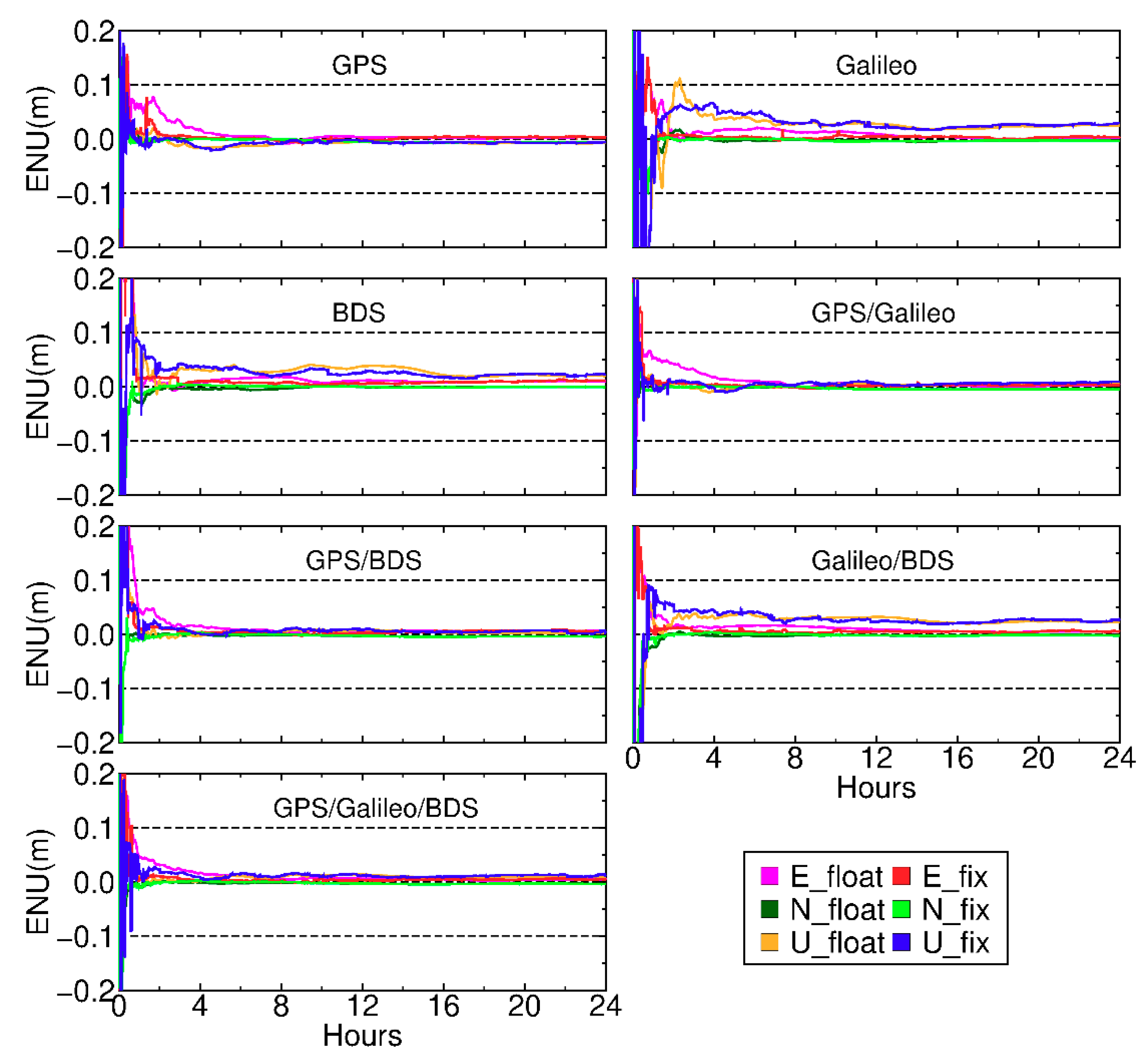
Figure 10 presents the errors in the fixed and float solutions in the east (E), north (N) and up (U) components for the seven systems at station KAT1 on DOY 324, 2018. For GPS, the fixed solution in the horizontal direction has a faster convergence rate than the float solution, and the accuracy after convergence is also higher. The fixed solution in the U direction exhibits slightly faster convergence than the float solution, but the accuracy after convergence is basically the same. In terms of Galileo and BDS, when the ambiguity is fixed to the correct integer, the horizontal direction converges to the truth value quickly, and the accuracy of the fixed solution in the U direction is equal to that of the float solution, with a systematic deviation of about 3 cm. In the case of the dual-system combination, the convergence rate of the horizontal fixed solution is much larger than that of the float solution, especially for the E direction. After convergence, the fixed solution accuracy of the three dual-systems is about 1 cm in the horizontal direction, within 2 cm for GPS/Galileo and GPS/BDS, and 4 cm for Galileo/BDS in the U direction. With respect to the GPS/Galileo/BDS integrated system, the convergence speed and accuracy of the fixed solution in all three directions are faster than that of the float solution. After convergence, the horizontal accuracy of the fixed solution is within 1 cm, some even around 5 mm, while for the U direction it is about 1.5 cm.
To sum up, the convergence speed and accuracy of the seven system fixed solutions in the horizontal direction are better than those of the float solution. For the U direction, the convergence speed of the fixed solution is slightly faster than the float solution, but the accuracy after convergence is basically the same. In the single-system, the GPS fixed and float solutions have the best accuracy and fastest convergence rate, while Galileo and BDS are basically equivalent. In the dual-system, GPS/Galileo performs the best, followed by GPS/BDS, and Galileo/BDS exhibits the worst. In addition, the convergence speed and accuracy of the dual-system combination is superior to the corresponding single-system. The triple-system shows the best performance, since the combined system leads to an increase in the satellite number and an enhancement of the satellite spatial structure, thereby improving the convergence speed and accuracy.
Figure 11 depicts the fixed results of seven systems in the E, N, and U components, respectively. It can be seen that in the E direction, the convergence rate of the Galileo fixed solution is the slowest, followed by BDS, and a slight fluctuation occurs after the convergence of GPS, which indicates that the single system fixed solution is relatively slow and unstable. The convergence speed of GPS/Galileo/BDS is basically the same as that of GPS/Galileo and GPS/BDS. After convergence, the accuracies of the seven systems are all basically within 1 cm. Similar to the E direction, Galileo converges the slowest in the N direction, followed by BDS, while the accuracies of the seven systems after convergence are basically the same. In addition, the convergence speed and accuracy of the seven systems in the N direction are all better than those in the E direction. With respect to the U direction, the convergence speed and accuracy of each system are obviously stratified. GPS/Galileo/BDS and GPS/BDS show the fastest convergence speed and highest accuracy, followed by GPS/Galileo, the GPS single system ranks the fourth, and finally, the Galileo/BDS, BDS and Galileo, respectively. Generally speaking, the convergence speed of the triple-system is obviously faster than that of the dual-systems, and the dual-systems are significantly faster than that of the single system. Therefore, the combined system is of great help to improve the convergence rate.
Figure 12 shows the average root mean square (RMS) of the float PPP solution for the seven systems in the E, N, and U components from DOY 321 to 350, 2018. In the E direction, for a single system, Galileo has the highest accuracy, followed by GPS, and BDS exhibits the worst accuracy of about 1.7 cm. For dual-systems, GPS/BDS performs the worst, Galileo/BDS ranks the second, and GPS/Galileo shows the highest accuracy of about 7 mm. It is also worth noting that the accuracy of the triple-system combination for some stations are not the highest, such as CEDU, DARW, KAT1, and so forth, but basically the same as the accuracy of GPS/Galileo. With respect to the N direction, the accuracy of BDS in all stations is about 1 cm, and the accuracy of GPS/BDS/Galileo is up to 5 mm, while the accuracies of other systems are basically the same. In the U direction, there is a very obvious phenomenon, the accuracy of the GPS single system in all stations is the highest, ranging from 0.5 to 1.5 cm, while the accuracy of BDS is the worst, between 3.5 and 6.5 cm.
The average RMS of the fixed PPP solution for seven systems from DOY 321 to 350, 2018 are shown in Figure 13. In the E direction, except for station CEDU, YARR obtained from BDS, and station DARW, KAT1 from GPS, all the rest stations show an accuracy of less than 1 cm under the seven systems. In addition, the accuracy of the fixed solution for these eight stations under all the seven systems is greatly improved compared with the float solution (Figure 12). In the N direction, the accuracy of all stations for the seven systems is about 5 mm except for station BAKO, HKSL from Galileo and station CEDU, YAR3, YARR from BDS. Besides, it can be seen that except for BDS, the accuracy between other systems of all stations have little difference and is also relatively uniform. With respect to the U component, the precision of the seven systems is quite different. The accuracy of BDS is still the worst, followed by Galileo and Galileo/BDS, while GPS shows the best performance. Among the eight stations, the accuracy of GPS/Galileo, GPS/BDS and GPS/Galileo/BDS exhibits little difference.
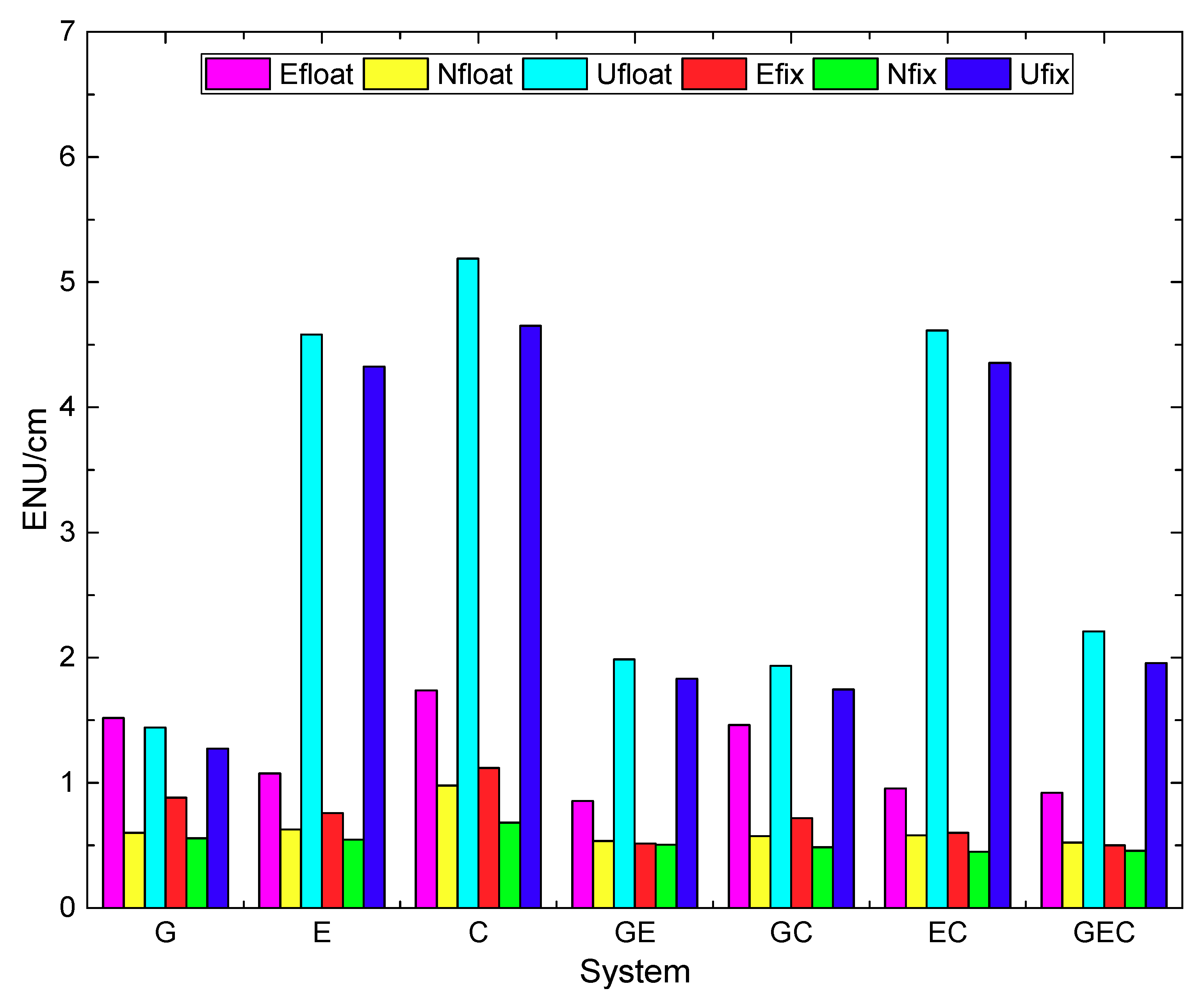
Figure 14 provides a more intuitive comparison of float and fixed PPP solution for different systems. Table 1 shows the average RMS of float and fixed PPP solution for seven systems from DOY 321 to 350, 2018. It is obvious that the average RMS value of the fixed solution is smaller than that of the float solution for all three directions. Among them, the E direction improves the most, followed by the U direction, while the N direction exhibits the smallest improvement. The GPS/Galileo/BDS in the E and N directions show the smallest RMS value of 0.92 cm, 0.52 cm and 0.50 cm, 0.46 cm for the float and fixed solutions, respectively, while the GPS single system exhibits the highest precision in the U component, with the RMS of 1.44 cm and 1.27 cm. Compared with single system, the accuracy of the dual-system and triple-system in the horizontal direction are improved obviously. The precision of GPS/BDS, GPS/Galileo and GPS/Galileo/BDS in the U direction is also greatly improved compared with Galileo and BDS. However, Galileo/BDS shows little improvement. This is mainly due to the poor accuracy of the single Galileo and BDS in the U direction.
6. Discussions
The combined system is conducive to enhance the satellite spatial structure, reduce the convergence time and enhance the stability of the positioning results. Up to now, research on combined PPP fixed solutions mainly focus on the GPS/BDS, and a few studies involve Galileo. Since GPS, Galileo and BDS all belong to code division multiple access (CDMA) constellations, and since Galileo and BDS are in continuous construction, it is necessary to systematically study and evaluate the PPP fixed solution of the combined GPS/BDS/Galileo. Moreover, the time-varying characteristics of FCB of each system also need to be analyzed in detail. The result of this paper shows that Galileo WL FCB has the highest precision, and the accuracy of GPS WL FCB and BDS non-GEO FCB is basically the same, second only to Galileo. With the exception of BDS GEO NL FCB, the NL FCBs of the other three systems have approximately the same accuracy.
With the continuing development of BDS and Galileo, more satellites and more frequency resources will be available in the future. It is expected that multi-frequency and multi-GNSS will be of great significance to shorten the convergence time and enhance the stability of the system. Therefore, it is necessary to conduct further research on multi-GNSS combination with ambiguity resolution once the new satellite comes into orbit.
7. Conclusions
This paper investigates the method of GPS/Galileo/BDS precise point positioning with ambiguity resolution. The FCB estimation methods of the three systems are firstly elaborated. Then, the WL and NL FCB of GPS, Galileo and BDS are analyzed in detail.
Our experimental results show that the accuracies of WL FCB for GPS and BDS non-GEO satellites are basically the same, while Galileo WL FCB exhibits the highest stability. Most of GPS, Galileo, and BDS non-GEO NL FCB ranges within 0.1 cycles, with little difference among them. Due to the poor accuracy, BDS GEO WL and NL FCB cannot be used for PPP AR. Therefore, it is appropriate to estimate WL FCB per day and NL FCB per 5 min for PPP AR.
In order to analyze the positioning accuracy, the number of global observable satellites and PDOP values of the single and integrated systems are simulated and analyzed. Results show that GPS and Galileo satellites are more evenly distributed around the world, with 8–9 and 5–6 satellites visible in the middle and low latitudes. BDS has a large number of satellites in the Asia-Pacific region, in general 8–15 satellites can be observed, while only 0–3 satellites can be observed in the corresponding Western Hemisphere. The global visible number of satellite and the PDOP value of the triple-system are superior to the dual-system, and the dual-system is better than the single-system.
Finally, with the estimated FCB products, the performance of the float and fixed solution for the single and integrated systems are evaluated. As can be seen, the convergence speed and accuracy of the fixed solutions for the seven systems are all better than that of the float solutions, especially for the horizontal direction. The GPS/Galileo/BDS combined system exhibits the smallest average RMS values in the E and N directions, being 0.92 cm, 0.52 cm and 0.50 cm, and 0.46 cm for the float and fixed solution, respectively, while GPS shows the highest accuracy in the U direction, with average RMS of 1.44 cm and 1.27 cm.
Author Contributions
X.L. conceived the study and wrote the original manuscript; X.L., H.C., and R.X. performed the experiments; C.S. and X.Z. analyzed the data; X.L., W.J., and W.Z. reviewed the paper, all authors read and contributed to subsequent draft.
Funding
The contribution of data from MGEX is appreciated. This research is supported by the National Key Research and Development Program of China (2018YFC1503600), the National Science Foundation for Distinguished Young Scholars of China (Grant No.41525014), the Natural Science Innovation Group Foundation of China (No. 41721003), the Major Technology Innovation Project of Hubei Province of China (2018AAA066), and Youth Fund of the National Natural Science Fund project (41704030).
Conflicts of Interest
The authors declare no conflict of interest.
References
- Zumberge, J.F.; Heflin, M.B.; Jefferson, D.C.; Watkins, M.M.; Webb, F.H. Precise point positioning for the efficient and robust analysis of GPS data from large networks. J. Geophys. Res. Solid Earth 1997, 102, 5005–5017. [Google Scholar] [CrossRef]
- Kouba, J.; Héroux, P. Precise point positioning using IGS orbit and clock products. GPS Solut. 2001, 5, 12–28. [Google Scholar] [CrossRef]
- Li, X.; Dick, G.; Ge, M.; Helse, S.; Wickert, J.; Bender, M. Real-time GPS sensing of atmospheric water vapor: Precise point positioning with orbit, clock, and phase delay corrections. Geophys. Res. Lett. 2014, 41, 3615–3621. [Google Scholar] [CrossRef]
- Geng, J.; Guo, J.; Chang, H.; Li, X. Toward global instantaneous decimeter-level positioning using tightly coupled multi-constellation and multi-frequency GNSS. J. Geod. 2019, 93, 977–991. [Google Scholar] [CrossRef]
- Gao, Y.; Chen, K. Performance analysis of precise point positioning using Real-time orbit and clock products. J. Glob. Position. Syst. 2004, 3, 95–100. [Google Scholar] [CrossRef]
- Le, A.Q.; Tiberius, C. Single-frequency precise point positioning with optimal filtering. GPS Solut. 2007, 11, 61–69. [Google Scholar] [CrossRef]
- Cai, C.; Gao, Y. Performance analysis of precise point positioning based on combined GPS and GLONASS. In Proceedings of the ION GNSS, 25–28 September 2007; pp. 858–865. [Google Scholar]
- Melgard, T.; Vigen, E.; Jong, K.D.; Lapucha, D.; Visser, H.; Oerpen, O. G2-The first real-time GPS and GLONASS precise orbit and clock service. In Proceedings of the International Technical Meeting of the Satellite Division of the Institute of Navigation, Savannah, GA, USA, 9 September 2001; Volume 5538, pp. 1885–1891. [Google Scholar]
- Li, X.; Zhang, X.; Guo, F. Study on precise point positioning based on combined GPS and GLONASS. In Proceedings of the ION GNSS, Savannah, GA, USA, 22–25 September 2009; pp. 2449–2459. [Google Scholar]
- Li, P.; Zhang, X. Modeling and Performance Analysis of GPS/GLONASS/BDS Precise Point Positioning. In Proceedings of the China Satellite Navigation Conference, Nanjing, China, 21–23 May 2014; pp. 251–263. [Google Scholar]
- Li, W.; Teunissen, P.J.G.; Zhang, B.; Verhagen, S. Precise point positioning using GPS and COMPASS observations. In Proceedings of the China Satellite Navigation Conference, Wuhan, China, 15–17 May 2013; pp. 367–378. [Google Scholar]
- Shen, X.; Gao, Y. Analyzing the impacts of Galileo and modernized GPS on precise point positioning. In Proceedings of the ION GPS, Portland, OR, USA; 2006; Volume 49, pp. 1532–1539. [Google Scholar]
- Cao, W.; Hauschild, A.; Steigenberger, P.; Langley, R.B.; Urquhart, L.; Santos, M. Performance evaluation of integrated GPS/GIOVE precise point positioning. In Proceedings of the ION NTM, San Diego, CA, USA, March 2010; pp. 540–552. [Google Scholar]
- Cai, C.; Gao, Y.; Pan, L.; Zhu, J. Precise point positioning with quad-constellations: GPS, BeiDou, GLONASS and Galileo. Adv. Space Res. 2015, 56, 133–143. [Google Scholar] [CrossRef]
- Teunissen, P.J.G.; Kleusberg, A. GPS Observation Equations and Positioning Concepts. In Lecture Notes in Earth Sciences: GPS for Geodesy; Springer: Berlin/Heidelberg, Germany, 1996; Volume 60, pp. 175–217. [Google Scholar]
- Gabor, M.J.; Nerem, R.S. GPS Carrier Phase Ambiguity Resolution Using Satellite-Satellite Single Differences. In Proceedings of the ION GPS 1999, Nashville, TN, USA, 14–17 September 1999; pp. 1569–1578. [Google Scholar]
- Gabor, M.J.; Nerem, R.S. Characteristics of Satellite-Satellite Single Difference Widelane Fractional Carrier Phase Biases. In Proceedings of the ION GPS 2000, Salt Lake City, UT, USA, 19–22 September 2000; pp. 396–406. [Google Scholar]
- Ge, M.; Gendt, G.; Rothacher, M.; Shi, C.; Liu, J. Resolution of GPS carrier-phase ambiguities in Precise Point Positioning (PPP) with daily observations. J. Geod. 2008, 82, 389–399. [Google Scholar] [CrossRef]
- Collins, P.; Lahaye, F.; Herous, P.; Bisnath, S. Precise point positioning with AR using the decoupled clock model. In Proceedings of the ION GNSS. Institute of Navigation, Savannah, GA, USA, 16–19 September 2008; pp. 1315–1322. [Google Scholar]
- Geng, J.; Teferle, F.N.; Shi, C.; Meng, X.; Dodson, A.H.; Liu, J. Ambiguity resolution in precise point positioning with hourly data. GPS Solut. 2009, 13, 263–270. [Google Scholar] [CrossRef]
- Geng, J.; Meng, X.; Alan, H.D.; Teferle, F.N. Integer ambiguity resolution in precise point positioning: Method comparison. J. Geod. 2010, 84, 569–581. [Google Scholar] [CrossRef]
- Li, P.; Zhang, X. Integrating GPS and GLONASS to accelerate convergence and initialization times of precise point positioning. GPS Solut. 2014, 18, 461–471. [Google Scholar] [CrossRef]
- Liu, Y.; Song, W.; Lou, Y.; Ye, S.; Zhang, R. GLONASS phase bias estimation and its PPP ambiguity resolution using homogeneous receivers. GPS Solut. 2017, 21, 427–437. [Google Scholar] [CrossRef]
- Liu, Y.; Ye, S.; Song, W.; Lou, Y.; Chen, D. Integrating GPS and BDS to shorten the initialization time for ambiguity-fixed PPP. GPS Solut. 2017, 21, 333–343. [Google Scholar] [CrossRef]
- Li, P.; Zhang, X.; Guo, F. Ambiguity resolved precise point positioning with GPS and BeiDou. J. Geod. 2017, 91, 25–40. [Google Scholar]
- Li, X.; Li, X.; Yuan, Y.; Zhang, K.; Zhang, X.; Wickert, J. Multi-GNSS phase delay estimation and PPP ambiguity resolution: GPS, BDS, GLONASS, Galileo. J. Geod. 2017, 92, 579–608. [Google Scholar] [CrossRef]
- Liu, X.; Jiang, W.; Li, Z.; Chen, H.; Zhao, W. Comparison of convergence time and positioning accuracy among BDS, GPS and BDS/GPS precise point positioning with ambiguity resolution. Adv. Space Res. 2019, 63, 3489–3504. [Google Scholar] [CrossRef]
- Melbourne, W.G. The case for ranging in GP S-based geodetic systems. In Proceedings of the First International Symposium on Precise Positioning with the Global Positioning System, Rockville, MD, USA, 15–19 April 1985. [Google Scholar]
- Wübbena, G. Software developments for geodetic positioning with GPS using TI-4100 code and carrier measurements. In Proceedings of the First International Symposium on Precise Positioning with the Global Positioning System, Rockville, MD, USA, 15–19 April 1985. [Google Scholar]
- Liu, J.; Ge, M. PANDA software and its preliminary result of positioning and orbit determination. Wuhan Univ. J. Nat. Sci. 2003, 8, 603. [Google Scholar]
- Blewitt, G. An automatic editing algorithm for GPS data. Geophys. Res. Lett. 1990, 17, 199–202. [Google Scholar] [CrossRef]
- Liu, X.; Jiang, W.; Chen, H.; Zhao, W.; Huo, L.; Huang, L.; Chen, Q. An analysis of inter-system biases in BDS/GPS precise point positioning. GPS Solut. 2019, 23, 116. [Google Scholar] [CrossRef]
- Kouba, J. A Guide to Using International GNSS Service (IGS) Products. 2009. Available online: http://igscb.jpl.nasa.gov/igscb/resource/pubs/UsingIGSProductsVer21.pdf (accessed on 15 January 2019).
- Hauschild, A.; Montenbruck, O.; Sleewaegen, J.M.; Huisman, L.; Teunissen, P. Characterization of Compass M-1 signals. GPS Solut. 2012, 16, 117–126. [Google Scholar] [CrossRef]
- Perello Gisbert, J.V.; Batzilis, N.; Risueno, G.L.; Rubio, J.A. GNSS payload and signal characterization using a 3 m dish antenna. In Proceedings of the ION GNSS, Nashville, TN, USA, 9 December 2012; pp. 347–356. [Google Scholar]
- Montenbruck, O.; Hauschild, A.; Steigenberger, P.; Hugentobler, U.; Riley, S. A COMPASS for Asia: First experience with the BeiDou-2 regional navigation system. In Proceedings of the Poster at IGS Workshop, Olsztyn, Poland, 23–27 July 2012. [Google Scholar]
- Montenbruck, O.; Rizos, C.; Weber, R.; Weber, G.; Neilan, R.; Hugentobler, U. Getting a grip on multi-GNSS—the international GNSS service MGEX campaign. GPS World 2013, 24, 44–49. [Google Scholar]
- Wanninger, L.; Beer, S. BeiDou satellite-induced code pseudorange variations: Diagnosis and therapy. GPS Solut. 2015, 19, 639–648. [Google Scholar] [CrossRef] [Green Version]
Figure 1.
Geographic distribution of the reference network. Red triangles denote the 160 stations used for GPS/Galileo/BDS FCB estimation, while yellow stars denote the eight stations used to evaluate the performance of the combined systems.
Figure 1.
Geographic distribution of the reference network. Red triangles denote the 160 stations used for GPS/Galileo/BDS FCB estimation, while yellow stars denote the eight stations used to evaluate the performance of the combined systems.

Figure 2.
GPS WL FCB from DOY 321 to 350, 2018, referenced to G01.
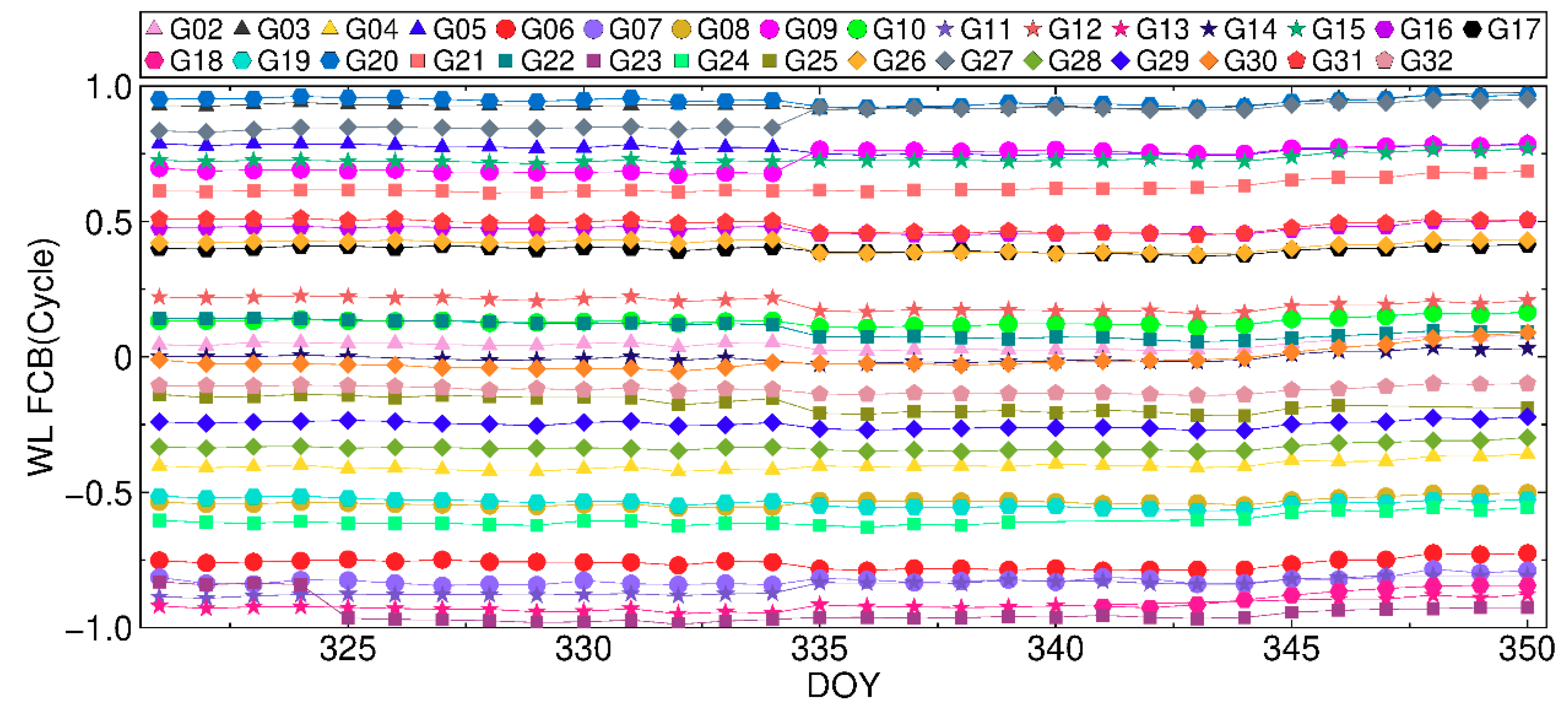
Figure 3.
GPS NL FCB on DOY 328, 2018, referenced to G01.

Figure 4.
Galileo WL FCB from DOY 321 to 350, 2018, referenced to E01.
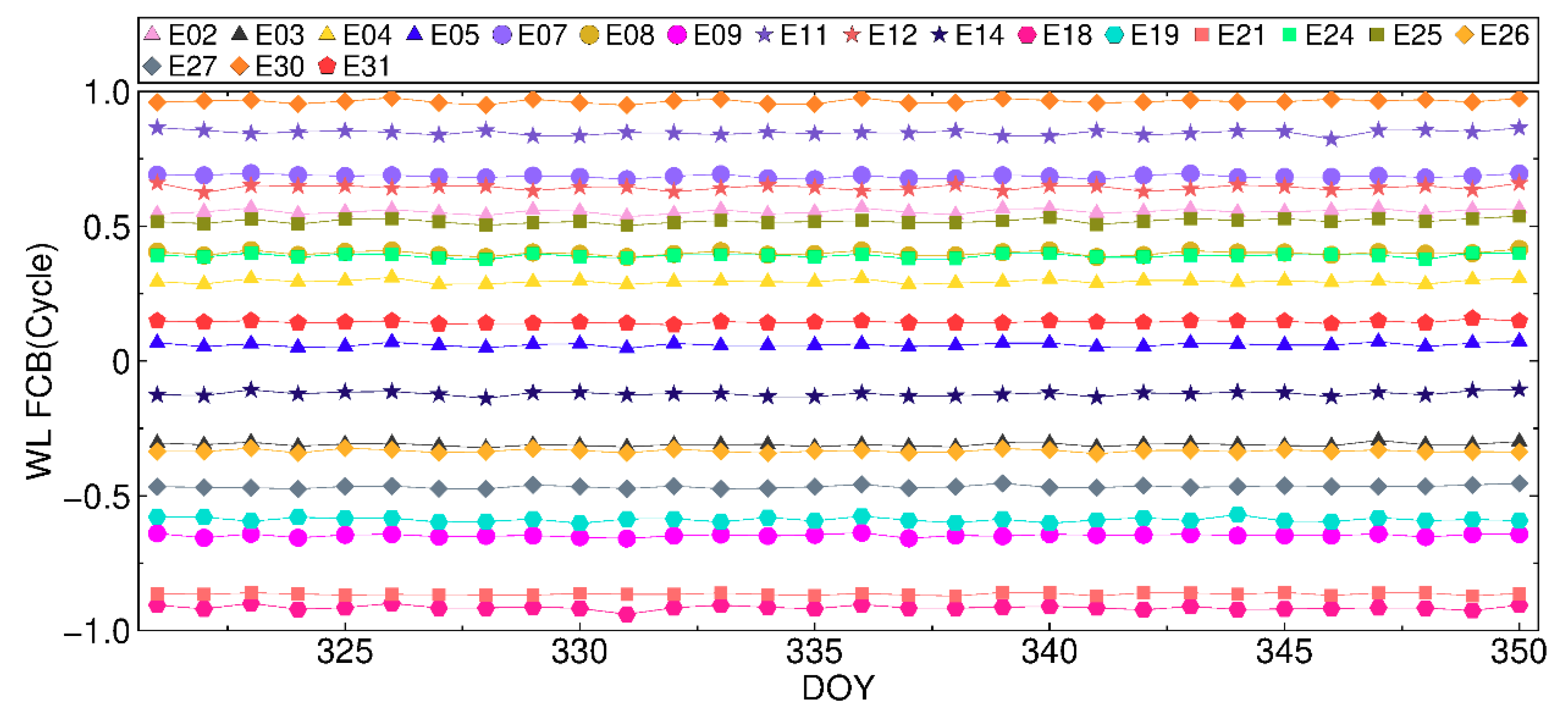
Figure 5.
Galileo NL FCB on DOY 328, 2018, referenced to E01.
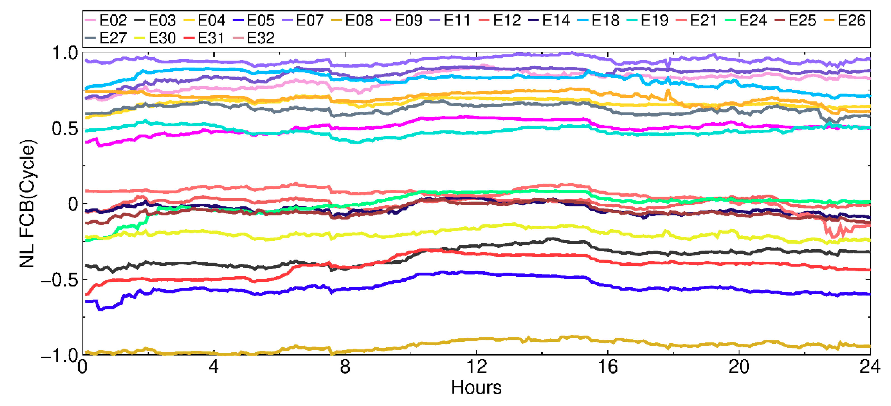
Figure 6.
BDS WL FCB from DOY 321 to 350, 2018. Top panel: BDS GEO. Bottom panel: BDS non-GEO. C02 and C06 are taken as the reference for BDS GEO and non-GEO respectively.
Figure 6.
BDS WL FCB from DOY 321 to 350, 2018. Top panel: BDS GEO. Bottom panel: BDS non-GEO. C02 and C06 are taken as the reference for BDS GEO and non-GEO respectively.
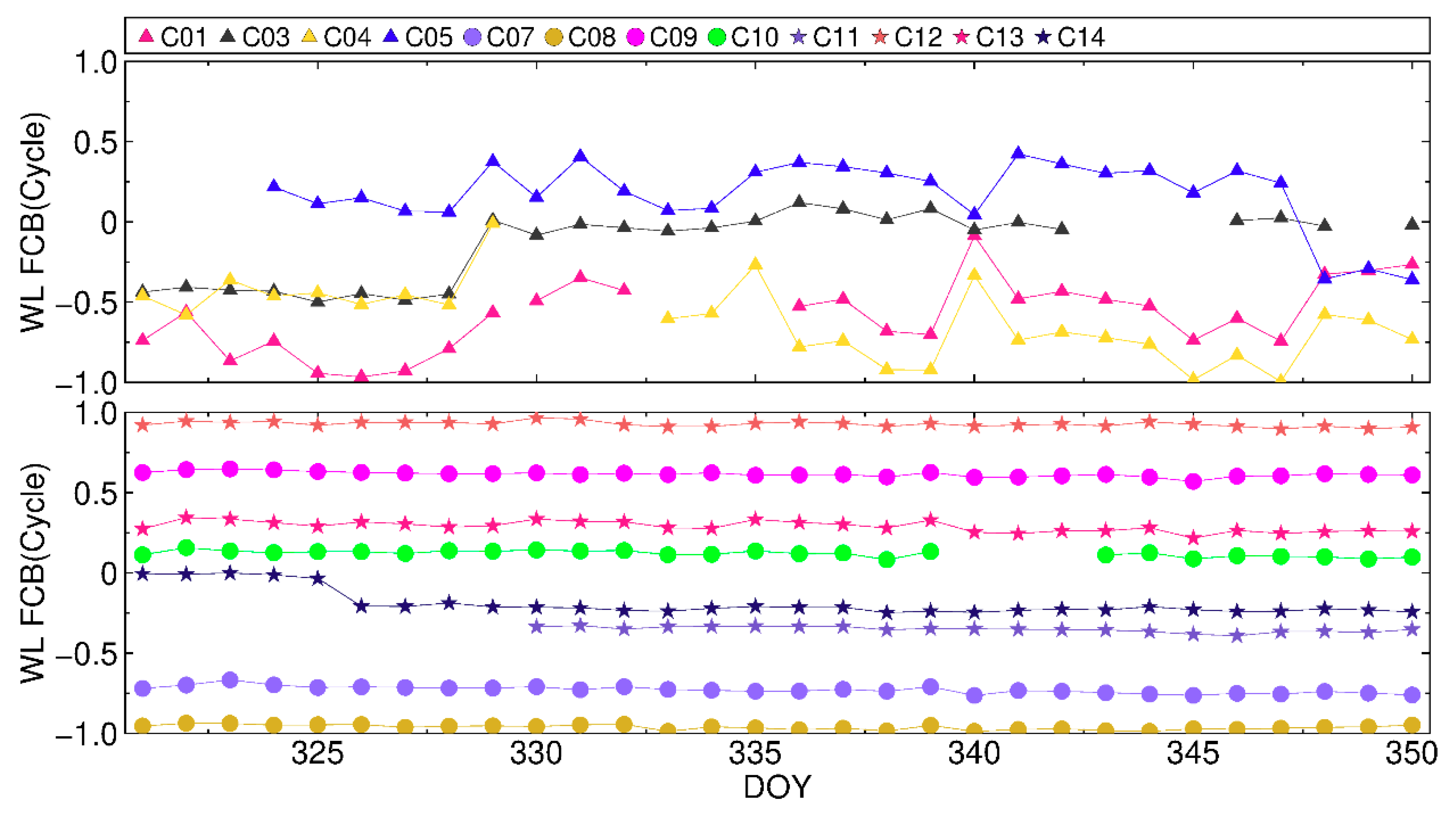
Figure 7.
BDS NL FCB on DOY 328, 2018. Top panel: BDS GEO. Bottom panel: BDS non-GEO. C02 and C06 are taken as the reference for BDS GEO and non-GEO respectively.
Figure 7.
BDS NL FCB on DOY 328, 2018. Top panel: BDS GEO. Bottom panel: BDS non-GEO. C02 and C06 are taken as the reference for BDS GEO and non-GEO respectively.
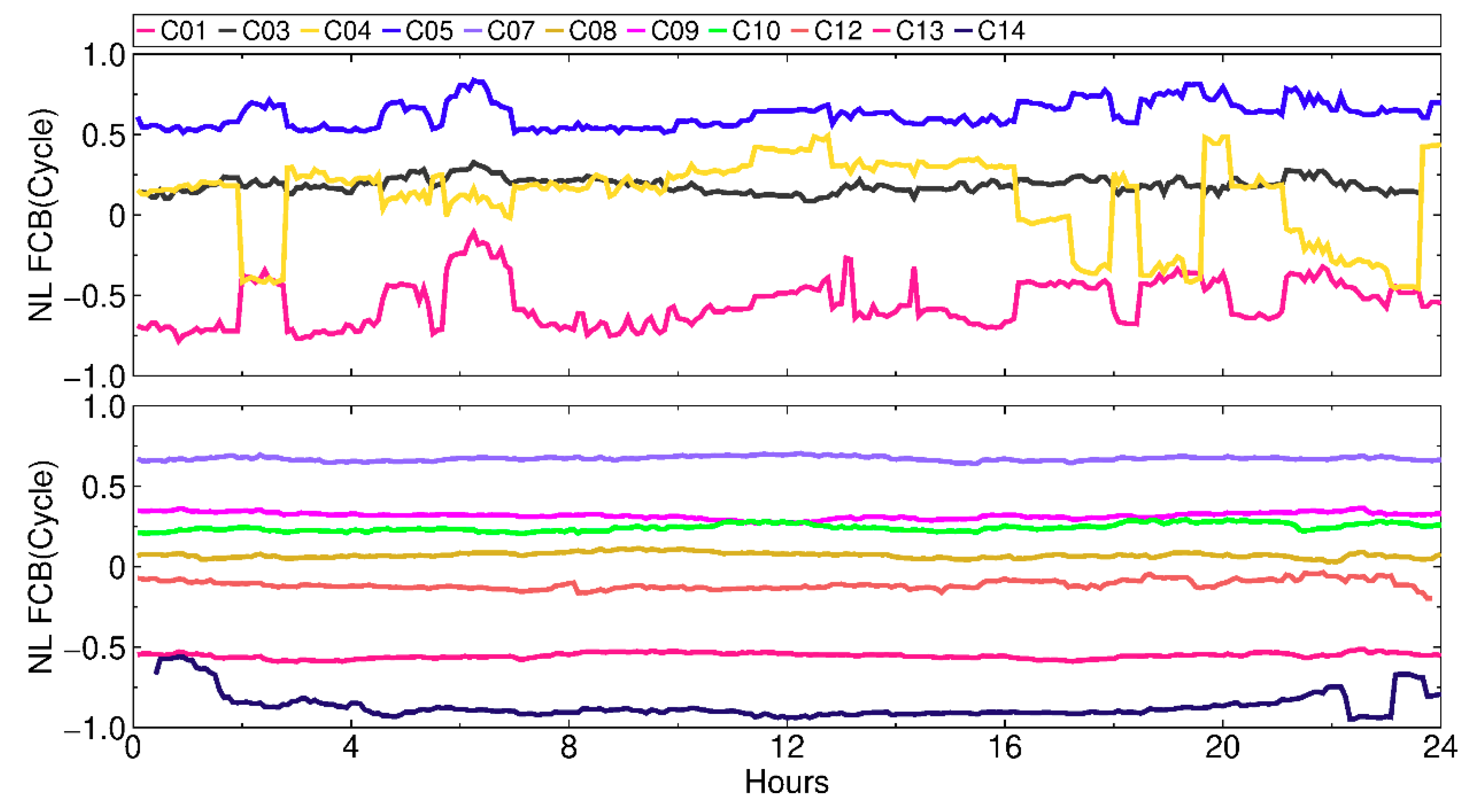
Figure 8.
Global distribution of the visible satellite number for seven different constellation combinations on DOY 321, 2018.
Figure 8.
Global distribution of the visible satellite number for seven different constellation combinations on DOY 321, 2018.
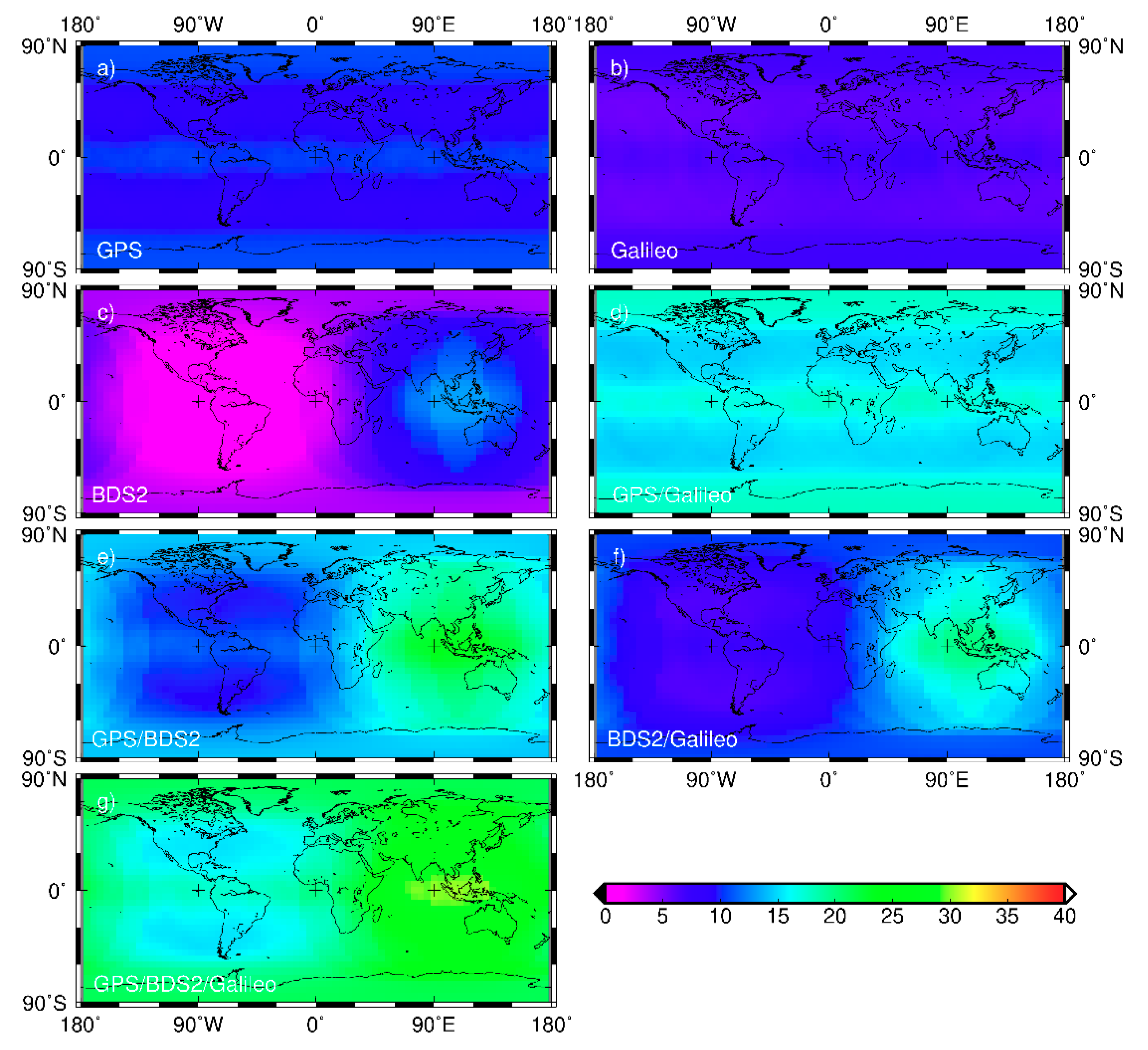
Figure 9.
Global distribution of the satellite PDOP values for seven different constellation combinations on DOY 321, 2018.
Figure 9.
Global distribution of the satellite PDOP values for seven different constellation combinations on DOY 321, 2018.

Figure 10.
Comparison of the float and fixed PPP results from single-system and combined solutions in the E, N, and U components, respectively, at station KAT1 on DOY 324, 2018.
Figure 10.
Comparison of the float and fixed PPP results from single-system and combined solutions in the E, N, and U components, respectively, at station KAT1 on DOY 324, 2018.

Figure 11.
Comparison of the fixed results for the seven systems in the E, N, and U components, respectively, at station KAT1 on DOY 324, 2018.
Figure 11.
Comparison of the fixed results for the seven systems in the E, N, and U components, respectively, at station KAT1 on DOY 324, 2018.
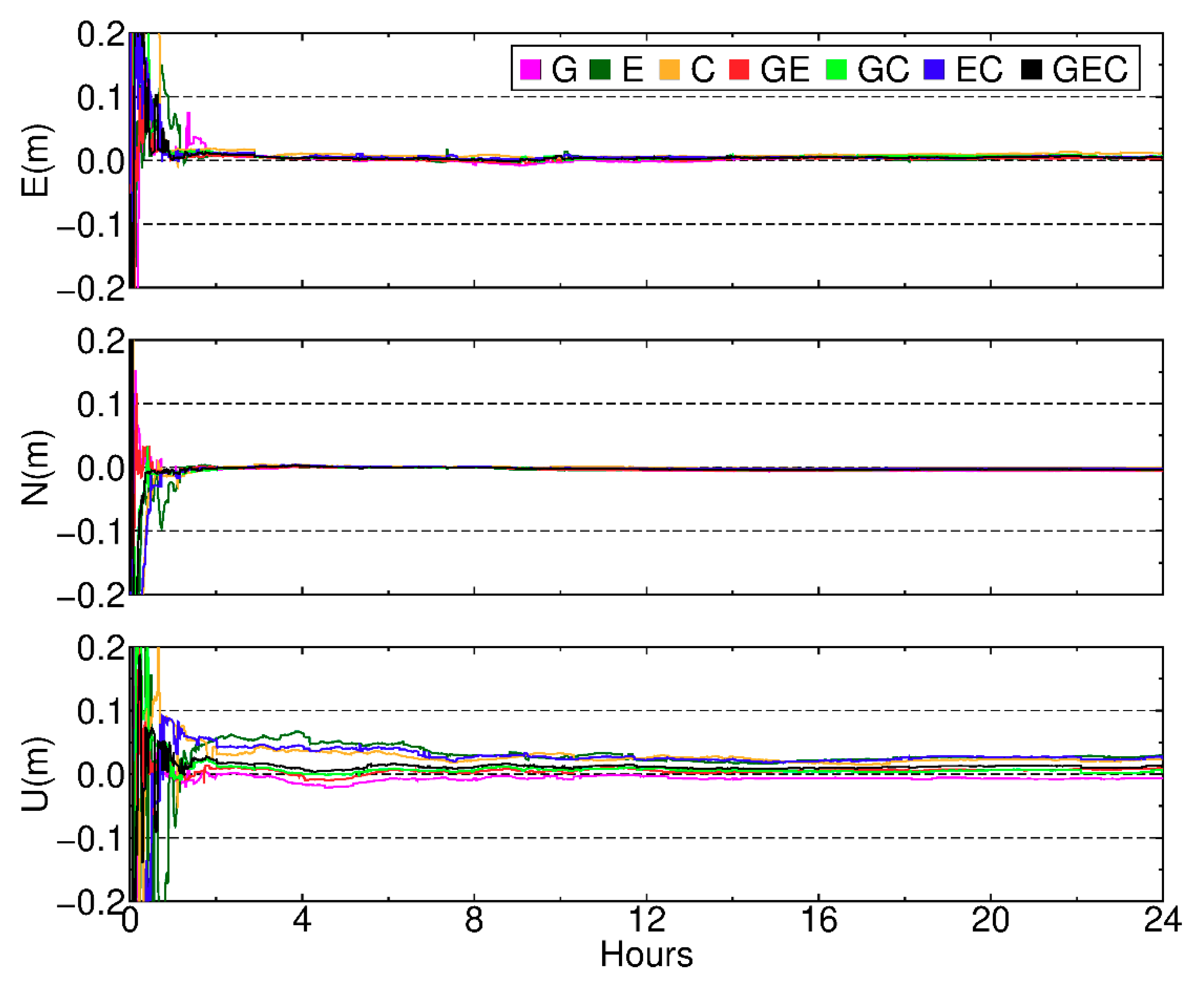
Figure 12.
The average RMS of float PPP solution from DOY 321 to 350, 2018.

Figure 13.
The average RMS of the fixed PPP solution from DOY 321 to 350, 2018.

Figure 14.
The average RMS of float and fixed PPP solution for seven systems from DOY 321 to 350, 2018.
Figure 14.
The average RMS of float and fixed PPP solution for seven systems from DOY 321 to 350, 2018.

Table 1.
The average RMS of float and fixed PPP solution for seven systems (unit: cm).
| System | Efloat | Nfloat | Ufloat | Efix | Nfix | Ufix |
|---|---|---|---|---|---|---|
| G | 1.52 | 0.60 | 1.44 | 0.88 | 0.56 | 1.27 |
| E | 1.08 | 0.63 | 4.58 | 0.76 | 0.55 | 4.33 |
| C | 1.74 | 0.98 | 5.19 | 1.12 | 0.68 | 4.65 |
| GE | 0.86 | 0.53 | 1.98 | 0.51 | 0.50 | 1.83 |
| GC | 1.46 | 0.57 | 1.93 | 0.72 | 0.49 | 1.75 |
| EC | 0.95 | 0.58 | 4.61 | 0.60 | 0.45 | 4.36 |
| GEC | 0.92 | 0.52 | 2.21 | 0.50 | 0.46 | 1.96 |
© 2019 by the authors. Licensee MDPI, Basel, Switzerland. This article is an open access article distributed under the terms and conditions of the Creative Commons Attribution (CC BY) license (http://creativecommons.org/licenses/by/4.0/).
Share and Cite
MDPI and ACS Style
Liu, X.; Chen, H.; Jiang, W.; Xi, R.; Zhao, W.; Song, C.; Zhou, X. Modeling and Assessment of GPS/Galileo/BDS Precise Point Positioning with Ambiguity Resolution. Remote Sens. 2019, 11, 2693. https://doi.org/10.3390/rs11222693
AMA Style
Liu X, Chen H, Jiang W, Xi R, Zhao W, Song C, Zhou X. Modeling and Assessment of GPS/Galileo/BDS Precise Point Positioning with Ambiguity Resolution. Remote Sensing. 2019; 11(22):2693. https://doi.org/10.3390/rs11222693
Chicago/Turabian StyleLiu, Xuexi, Hua Chen, Weiping Jiang, Ruijie Xi, Wen Zhao, Chuanfeng Song, and Xingyu Zhou. 2019. "Modeling and Assessment of GPS/Galileo/BDS Precise Point Positioning with Ambiguity Resolution" Remote Sensing 11, no. 22: 2693. https://doi.org/10.3390/rs11222693
Note that from the first issue of 2016, this journal uses article numbers instead of page numbers. See further details here.