Article

Analysis of Parameters for the Accurate and Fast Estimation of Tree Diameter at Breast Height Based on Simulated Point Cloud

1
College of Science, Beijing Forestry University, Beijing 100083, China
2
College of Land Science and Technology, China Agricultural University, Beijing 100083, China
3
Key Laboratory of Remote Sensing for Agri-Hazards, Ministry of Agriculture, Beijing 100083, China
4
Department of Microbiology and Plant Biology, Center for Spatial Analysis, University of Oklahoma, Norman, OK 73019, USA
*
Author to whom correspondence should be addressed.
Remote Sens. 2019, 11(22), 2707; https://doi.org/10.3390/rs11222707
Submission received: 12 September 2019 / Revised: 28 October 2019 / Accepted: 13 November 2019 / Published: 19 November 2019
(This article belongs to the Special Issue Virtual Forest)

Abstract

:
Terrestrial laser scanning (TLS) is a high-potential technology in forest surveys. Estimating the diameters at breast height (DBH) accurately and quickly has been considered a key step in estimating forest structural parameters by using TLS technology. However, the accuracy and speed of DBH estimation are affected by many factors, which are classified into three groups in this study. We adopt an additive error model and propose a simple and common simulation method to evaluate the impacts of three groups of parameters, which include the range error, angular errors in the vertical and horizontal directions, angular step width, trunk distance, slice thickness, and real DBH. The parameters were evaluated statistically by using many simulated point cloud datasets that were under strict control. Two typical circle fitting methods were used to estimate DBH, and their accuracy and speed were compared. The results showed that the range error and the angular error in horizontal direction played major roles in the accuracy of DBH estimation, the angular step widths had a slight effect in the case of high range accuracy, the distance showed no relationship with the accuracy of the DBH estimation, increasing the scanning angular width was relatively beneficial to the DBH estimation, and the algebraic circle fitting method was relatively fast while performing DBH estimation, as is the geometrical method, in the case of high range accuracy. Possible methods that could help to obtain accurate and fast DBH estimation results were proposed and discussed to optimize the design of forest inventory experiments.

Graphical Abstract

1. Introduction

Forests are the dominant terrestrial ecosystem on the Earth and are closely related to human production and life [1]. Monitoring forest biomass is one of the most important ways to understand the changes in forests and analyze the relationship between humans and the natural environment. As the dominant part of forest biomass, tree biomass can help to estimate and verify forest biomass.
The diameter of a tree at breast height (DBH) is one of the most common and important field measurements in forest inventories and is indispensable for accurately estimating timber volume and tree biomass. Traditionally, DBH can be manually measured by using a girthing tape or calipers. In recent decades, some new methods have been used to measure DBH, such as electrical calipers and laser scanners [2,3].
Terrestrial laser scanning (TLS) instruments generate high-density point cloud data for trees with high speed and high precision, which provides the basis for estimating the structural attributes of trees. In recent years, TLS has been widely used in forest inventories and has attracted increasing attention. Many attributes of trees of some species have been estimated by using in-situ data from TLS instruments, such as the DBH [4,5,6,7], tree height [2,8,9], aboveground biomass [10,11,12,13] and leaf area index (LAI) [6,14,15]. Compared with the traditional measurement of DBH which is usually labor intensive and time consuming in natural forests, DBH estimation based on point cloud data improves our ability to achieve fast and automatic results. Many DBH estimating methods have been proposed, and related experiments have been carried out [2,4,16]. Accurate DBH estimation based on point cloud data has remained an important issue in recent years [17,18,19,20].
Some studies have investigated several factors that affect the accuracy of DBH estimation using data collected in the fields in the past decade. For example, Maas et al. [2] compared the accuracy of DBH estimation by using two kinds of TLS instruments, RIEGL LMS-420i and FARO LS 800 HE80. Lovell et al. [5] reported DBH estimation by using Echidna instruments and discussed the impacts of beam divergence and angular step width. By using a FARO photon 120 instrument, Pueschel et al. [21] discussed the impacts of the scan mode on the DBH estimation of Beech and Douglas fir and analyzed the accuracies of the DBH estimation of three circle fitting methods. Pueschel [22] also evaluated the impacts of the angular step width and scan speed on DBH estimation. In practice, because of the diversity of TLS instruments, field scanning parameters and estimating methods, it is a challenge to compare the results, rank the performances of the methods and further improve the speed and accuracy of DBH estimation. Therefore, there is interest in considering the impacts of system parameters, scanning parameters and estimating methods, which can be used to improve the speed and accuracy of DBH estimation in most circumstances.
Numerical simulation has been used to investigate the effects of some factors of TLS. Pesci et al. [16] concluded that the effective scanning angular resolution is related to the beamwidth and angular step width by using numerical simulation experiments on surface details recognition. However, a few simulation studies have been published on the accuracy of the DBH estimation. Bu and Wang simulated the point cloud data of tilting trunk slice to discuss the impacts of different angular resolutions [23]. Forsman et al. [18] analyzed the bias of cylinder diameter estimation with different beamwidths by using a multi-parameter simulator. However, these simulation experiments did not describe the effects of the error parameters, scanning parameters and estimating methods on DBH estimation, which remain to be qualitatively analyzed. Furthermore, the efficiency of the DBH estimation was also not discussed in these studies which is important in data processing.
The goal of this paper is to provide a thorough analysis of the effects of error parameters, scanning parameters and estimating methods on the accuracy and speed of DBH estimation. The paper is organized as follows: Section 2 describes the analysis method, which includes the simulation of point clouds of tree slices, DBH estimation and evaluation of the estimated error. Section 3 presents the analysis of the simulated point cloud data with different scanning parameters. Section 4 discusses the results and explores possible explanations. Section 5 concludes the experiments. The results from this study should help to improve experimental design to efficiently obtain more accurate DBH estimation.

2. Materials and Methods

2.1. In-Situ TLS and Simulation Data

The effects of various factors on DBH estimation can be analyzed by using either in-situ TLS measurements or simulated data. In-situ TLS measurement data have several issues. First, the diversity of TLS instruments makes the analysis difficult in field experiments. As we know that the accuracy of DBH estimates is affected by the attributes of TLS instruments, such as ranging method, error characteristics, laser wavelength, and beam divergence. Many types of TLS instruments have been used to obtain point cloud data from trees [24]. Some TLS instruments are commercial products [2,4,21,25], and others are integrated with laser scanners and sensors for scientific research [26,27,28]. These TLS instruments may have different attributes and error characteristics. Second, variable scanning parameters inhibit the comparison of results of different in-situ experiments. For example, different angular step widths in the horizontal and vertical directions may be adopted in experiments, which results in different densities and amounts of data. Furthermore, the different densities and amounts of data may lead to different costs of storage space, computing powers and processing times, which result in different speeds and accuracies of DBH estimation. Third, the analysis can be hampered by other factors, such as the DBH estimating methods, environment and scanned trees in those experimental sites. For example, estimating DBH by using circle fitting methods is a basic and popular approach. However, different circle fitting methods also have characteristics [29] that may have different impacts on the accuracy and efficiency of DBH estimation.
In short, DBH estimation is affected by all of the abovementioned factors. It is not easy to distinguish the impacts of individual factors accurately for a specific TLS instrument in situ, let alone for so many types of TLS instruments. Although repeated experiments with different TLS instruments and different parameters are possible, it is costly, labor intensive and time consuming to perform many experiments and return to the test areas.
In this study, simulation data were used, as numerical simulation was a relatively flexible and economical way to provide some common sense for qualitative understanding accurate and fast DBH estimation methods. By using the numerical simulation method, common characteristics and key parameters of TLS instruments were analyzed without considering specific instrument types, and the simulated data was generated by using selected model parameters.

2.2. DBH Model Construction

In our method, the simulator was constructed by using three sets of parameters which were related to TLS instruments, field scanning, and tree trunks.
The first set of parameters was the error characteristics of the TLS instrument, which included range error and angular errors in vertical and horizontal directions. The TLS instrument was a complex and precise system, which included optics and electronics. Commercial TLS instruments were usually composed of a laser scanner and a camera, which obtained a large amount of information of objects present in the field of view (FOV) of TLS instrument, such as range, vertical angle, horizontal angle, intensity, amplitude, and RGB (red, green and blue colors). Some TLS instruments were also equipped with a Global Positioning System (GPS) receiver to assist in positioning. The components in the system affected each other. However, there were many types of TLS instruments and manufacturers rarely described the mechanism in detail for business reasons, which made it difficult to simulate the details of the system based on precise theory [18,21,30]. For most TLS instruments, a simple and common simulation method was very important and necessary. As key parameters, error characteristics described most of performance of point cloud data obtained using TLS instruments.
The second set of parameters was the scanning parameters of the TLS instrument, which were composed of step widths in the vertical and horizontal directions. Angular step widths defined the density of the point cloud data, which reflected the data acquisition ability of TLS instruments and was also the basis of accurate DBH estimation. A reasonable density of point cloud data preserved the accuracy of DBH estimation while reducing storage and computation costs. An excessive amount of data not only required extra storage space and computing power but also increased estimation processing time. However, less data reduced the accuracy of DBH estimation.
The third set of parameters was related to the trunk slice, which included the diameter, the thickness and the horizontal distance between the scanner and the tree position (the center point of the trunk slice) (Figure 1). In the real world, tree trunks were not standard cylinders and were affected by the surrounding environment. However, some assumptions about the trunk were proposed as follows to make the simulation easier to carry out. For the sake of simplification, the changes in terrain and tilting of trees were not considered in the simulation.
(a)
Each trunk was a cylinder that was perpendicular to the horizontal ground.
(b)
The virtual TLS scanner was placed at a height of 1.3 m, which is the exact height where the breast diameter was measured.
(c)
The position of the virtual TLS scanner was the origin (0, 0, 0) of the local coordinate system.
As shown in Figure 1, based on the previously mentioned three sets of parameters, the point cloud data of the trunk slice was generated and then used to perform DBH estimation. The estimated DBH was compared with the real DBH value, and the error was evaluated and analyzed. By changing only one parameter and keeping the rest of the parameters unchanged, we observed the impacts of factors on the speed and accuracy of DBH estimation.

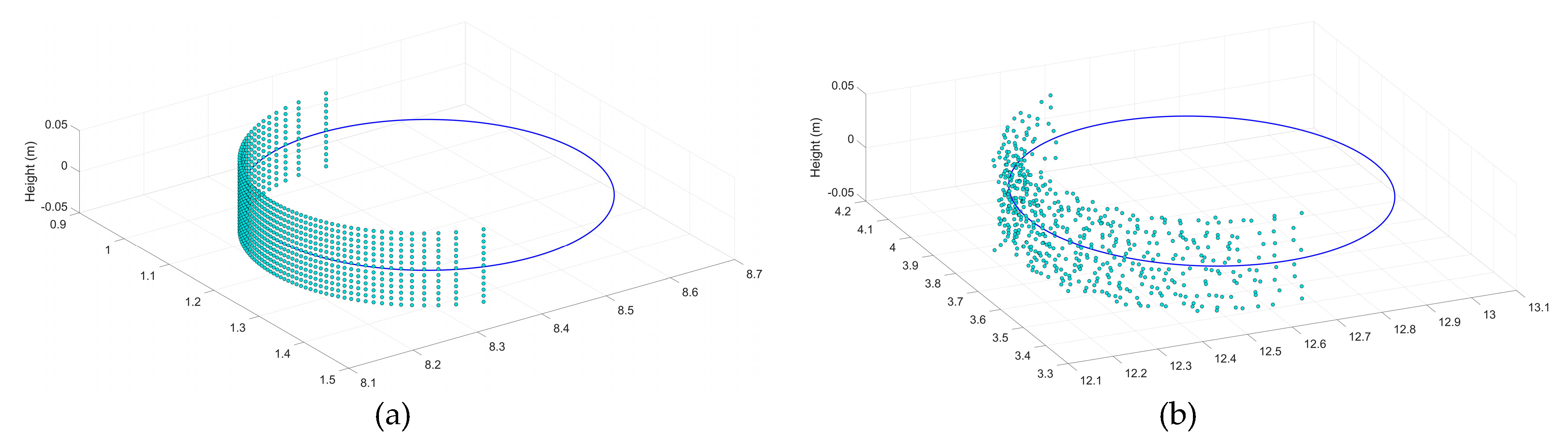
2.3. DBH Model Simulations

This paper addressed DBH estimation, which was achieved by using the spatial information from point cloud data. To simplify the simulation, other kinds of information that were not related to the estimation were not considered in the simulation. Therefore, only the spatial information of point cloud data was simulated, which helped to focus and simplify the problem. The raw observations of spatial information in TLS instruments were the range, horizontal angle and vertical angle [31]. Based on the scanning geometry (Figure 2), the ideal spatial information for the scanning points on an object were computed accurately [30]. For example, the spatial information of points A, B, and C (Figure 2) were calculated by using the values of range of the points and the angular step widths ( φ s , θ s ) , which were the scanning parameters in the simulation.
However, there were some errors in practical scanning. The range was affected by range error, and the two angles were affected by angular errors in two directions. Lichti performed extensive research on the error analysis of TLS instruments [30,31]. In his work, it was proposed that a modeling approach that augments the range and angular observations with additive model terms can be used to describe the systematic errors [31] and that each of the range error and angular errors is caused by a group of additive terms [31].
The abovementioned additive error model was adopted and simplified in our method. Due to the qualitative considerations concerning the commonality of many TLS instruments, a simple simulation method was favorable because it described the common experience. Then, the additive terms of each error were merged into one equivalent additive term in this paper.
r = r i d e a l + e r φ = φ i d e a l + e φ θ = θ i d e a l + e θ
where ( r i d e a l , φ i d e a l , θ i d e a l ) are the reference values of the range, horizontal angle, and vertical angle, respectively, ( r , φ , θ ) are measured values, and ( e r , e φ , e θ ) are the additive error terms. ( e r , e φ , e θ ) satisfy the Gaussian distributions, which have different variances ( σ r , σ φ , σ θ ) and zero mean values.
Based on the mechanism of the simulator and errors described above, the point cloud data of slices were generated. Two simulated slices with a thickness of 10 cm are shown in Figure 3. One is a slice without errors (the left panel in Figure 3), and the other is a slice with range and angular errors (the right panel in Figure 3). The circles with the real diameters and real positions are plotted in Figure 3 to illustrate the ideal positions of the slices.
The impacts of the factors should be evaluated and analyzed with a number of cases, which would help to obtain statistical results. To simulate the status of real-world scanning experiments, many trunk slices with random positions and diameters should be virtually scanned to generate point cloud data. The positions and diameters of slices were random values in their preset ranges, and they satisfied the uniform distributions. Meanwhile, in a real-world scanning experiment, the trees far from the scanner may be partially or totally blocked by the trees near the scanner. This occlusion effect could be simulated by using position and diameter information, which would result in variable arc lengths.
In our method, the following default simulation parameters were used in the simulation without special statements:
  • The range of DBH values was 0.1 m 0.4 m. The diameter of a slice was randomly chosen from this range.
  • The distance between the scanner and the real center of a slice was a random value in the range of 0.1 m 30 m.
  • The thickness of the slices was 0.1 m.
To observe and evaluate the impacts of the parameters, many controlled datasets with different parameters were generated. Different parameter settings were used to obtain different datasets, which resulted in different DBH estimation accuracies. The difference in these DBH estimations was analyzed to observe the impacts of a given parameter. The simulation parameters and their purposes are listed in Table 1. It should be noted that group six of the dataset was simulated with the thicknesses of 0.10 m, 0.15 m, 0.20 m and 0.25 m. In the experiment, 400 trunk slices were simulated for each parameter combination. Furthermore, there were 19,200 trunk slices in the total six group of datasets. The values of these parameters were reachable for most commercial TLS instruments and some laser scanners.

2.4. DBH Model Estimations

In the process of DBH estimation, two circle fitting methods were used to estimate the DBH values. One was the Levenberg–Marquardt method (LM method) [23,29], which was geometrical, and the other was the Taubin method, which is an algebraic method [21,29]. The accuracy and speed of the two circle fitting methods are discussed in the context of using the simulated datasets.
The spatial information of the simulated point cloud data can be used to fit a circle that is considered to have the same diameter as a trunk slice. In light of the aforementioned assumptions, the slice was perpendicular to the horizontal ground. The 3D point cloud data could be projected onto a horizontal plane. Then, the DBH estimation was carried out by using a circle fitting method.

2.5. Accuracy Assessment

Based on the estimated DBH values, the impacts of the factors were evaluated. However, data cleaning was needed since the DBH estimation results sometimes had serious deviations from the real values, and the estimation sometimes failed. The estimation failure was easy to define, and the outliers caused by deviations were detected. The DBH estimation results were not only affected by the fitting methods, but also affected by the number and distribution of points which were comprehensive results of related parameters used in the simulation. In practice, less points or bad distributions both may lead to serious deviations, or even failures.
In our method, a modified interquartile range (IQR) method was used, which defined outliers when the relative error was above Q3 + 3 * IQR. Q3 and Q1 were the values of the third quartile and first quartile, respectively, and IQR = Q3 − Q1. After the data were cleaned, they were used to perform the accuracy assessment.
Since the real DBH value was used as an input parameter, the evaluation of the DBH estimation for a single tree was easily performed by calculating the difference between the estimated DBH value and the real DBH value. For physical trees, the root mean square error (RMSE) value could be calculated and used to evaluate the effectiveness of the DBH estimation in an actual scanning experiment [10,13,21].
Although the RMSE value has been widely used in previous experiments, it was not very suitable for the comparison of experiments in which the trees differed in addition to the TLS instruments. On the one hand, the number of trees and the DBH values may have been different in these experiments, which could have affected the calculation of the RMSE. On the other hand, the range of diameters was not considered in the calculation of the RMSE. However, the same estimated difference means different estimation accuracies for different DBH values.
Similarly, the RMSE value was not a good index for evaluating the DBH estimation error in this paper. Rather than the RMSE value, the relative error was used in the paper:
E r r o r r e l a t i v e = A B S ( D B H e D B H r ) D B H r
with D B H e is the estimated value of DBH and D B H r is the real value of DBH.

3. Results

3.1. Performances of the Two Circle Fitting Methods

The performances of two representative circle fitting methods were observed and evaluated by using group one of the dataset. Keeping σ φ ( σ θ ) at 0 degrees and θ s ( φ s ) at 0.02 degrees, the relations between the real and estimated DBH values were illustrated (Figure 4) when σ r was assigned four gradually increasing values.
As shown in Figure 4a, the two methods had almost the same results, which were slightly underestimated when σ r was 0.02 m. As σ r increased, the estimated results were underestimated to a greater degree. However, when σ r was 0.15 m, overestimation occurred in the results of two methods in the DBH range of 0.1 m to 0.17 m. The DBH values were seriously overestimated by using the Taubin method (the estimated values were too large to show in the drawing area) in this range. The larger DBH values remained underestimated, and the results of the Taubin method were larger than the results of the LM method.
The time cost of the two methods was extensively analyzed (Figure 5). In general, the LM method cost more time than the Taubin method since the geometrical method included iterative computations. As σ r increased, the time cost of the LM method increased obviously.

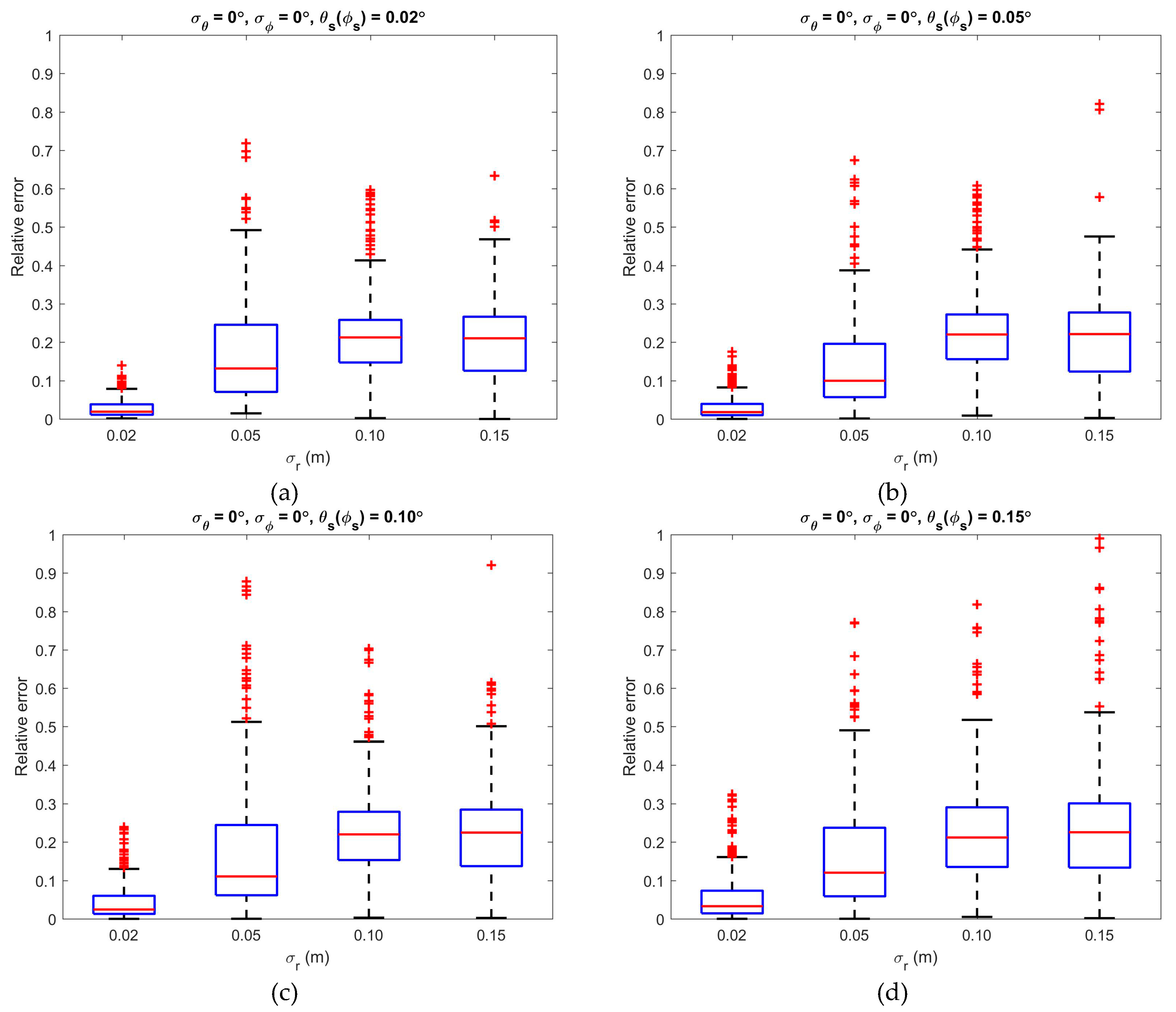
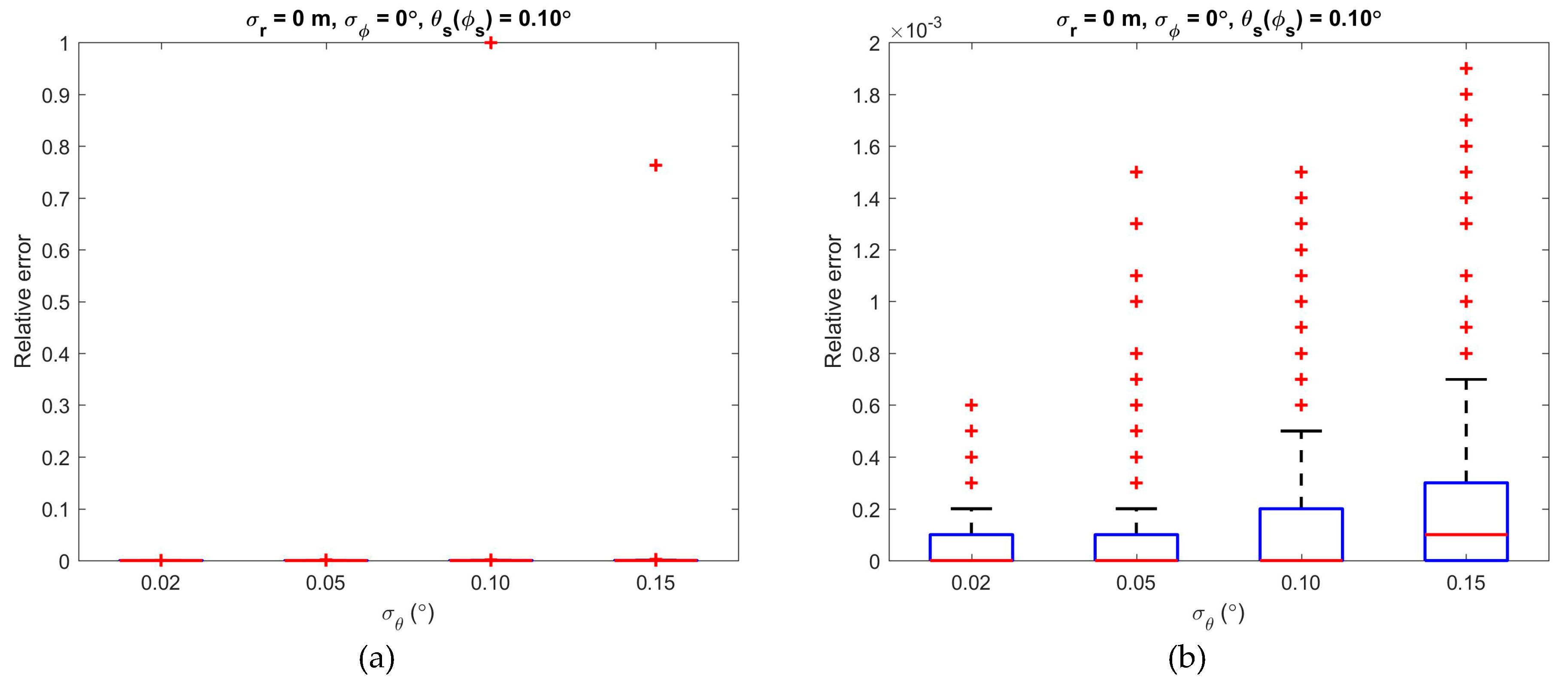
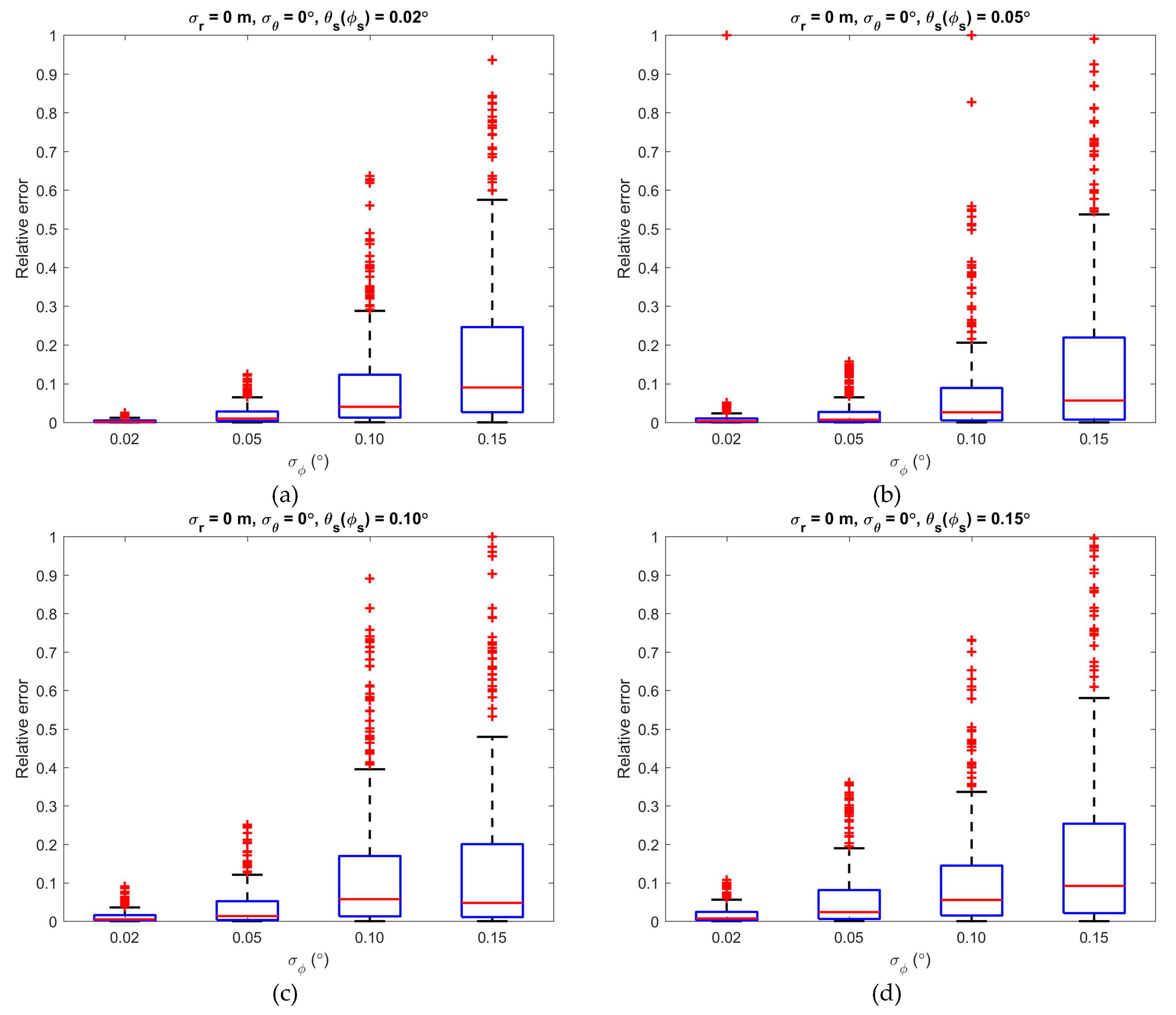
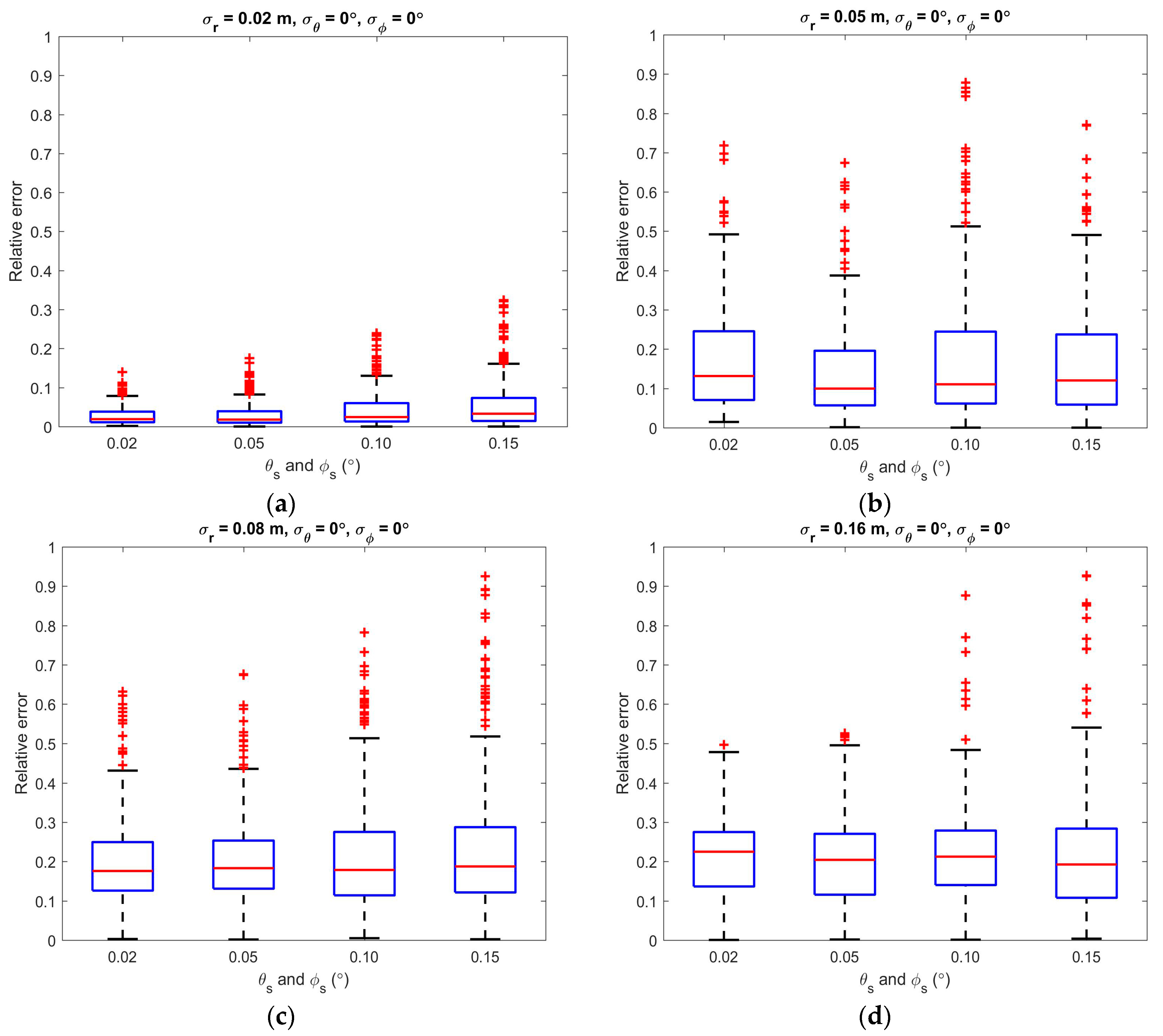
3.2. Impacts of the Error Parameters

The error parameters were divided into two categories for observation. One category was the range error, and the other contained the angular errors in the horizontal and vertical directions.
First, group two of the dataset was used to observe and evaluate the impacts of the range error. To remove the impacts of the angular errors, the values of σ φ and σ θ were set to 0 ° in the experiment. The value of σ r was set as 0.02 m, 0.05 m, 0.10 m, and 0.15 m in turn. The values of the angular step widths ( θ s and φ s ) were set to the same values, i.e., 0.02 ° , 0.05 ° , 0.10 ° , and 0.15 ° . Then, sixteen combinations of simulation parameters were used to simulate twenty datasets of point cloud data. There were four hundred slices in each dataset.
The previously mentioned data cleaning was performed to remove the slices that had no data due to occlusion or that caused outliers. For each value of θ s and φ s , five datasets with increasing σ r were processed. Then, the estimated DBH values were compared with the real DBH values, and the relative errors of the DBH estimation were calculated, the results of which were used to create the quartile figure (Figure 6). The trends in the four subfigures were similar. The relative error increased significantly when σ r was between 0.02 m and 0.10 m and then remained almost constant (Figure 6).
These figures represent the statistical results of the simulated datasets. Accurate DBH estimation results appeared in every dataset and accounted for different proportions of the overall estimation. More accurate results occurred when σ r was relatively smaller. Increasing θ s ( φ s ) increased the relative error.
Second, group three of the dataset was used to observe and evaluate the impacts of the angular error in the vertical direction. Keeping σ r at 0 m, σ φ at 0 degrees and θ s ( φ s ) at 0.10 degrees, the value of σ θ was set as 0.02 degrees, 0.05 degrees, 0.10 degrees, and 0.15 degrees in turn.
The impact of σ θ on the relative error was too small to be observed clearly (Figure 7a). However, even though the magnitude of the impact was very small, when the figure was magnified regionally, the increasing impact on the relative error with increasing σ θ was observed (Figure 7b).
Third, we observed and evaluated the impacts of the angular error in the horizontal direction by using group four of the dataset. Keeping σ r at 0 m, σ θ at 0 degrees, the values of σ φ and θ s ( φ s ) were set as 0.02 degrees, 0.05 degrees, 0.10 degrees, and 0.15 degrees in turn.
Unlike the angular error in the vertical direction, the impact of σ φ on the relative error can be seen clearly, and the relative error increased evidently with increasing σ φ (Figure 8). Moreover, a similar trend can be seen with different θ s ( φ s ) values, and no significant changes were observed when θ s and φ s changed.

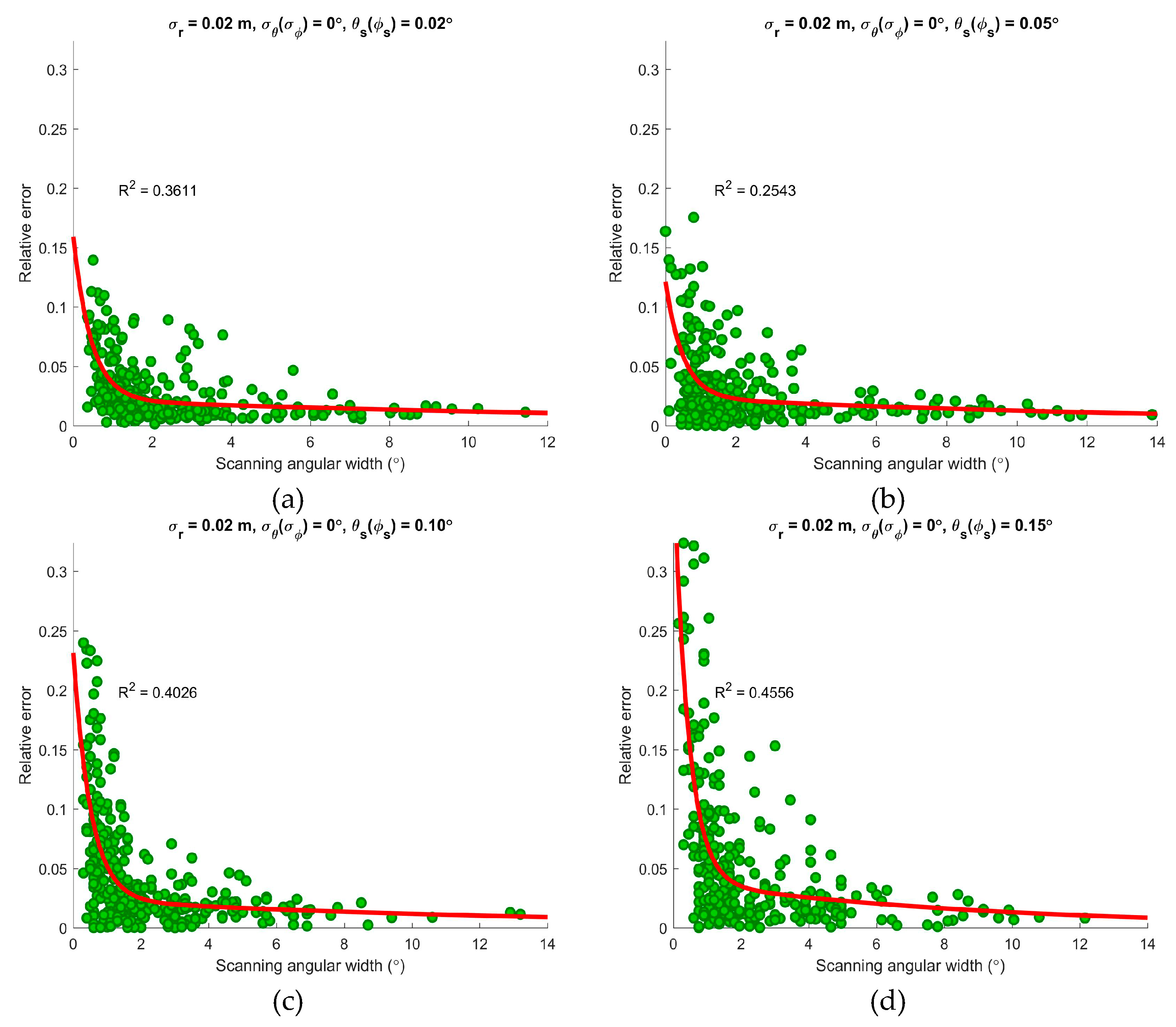
3.3. Impacts of the Angular Step Widths

Similarly, group two of the dataset was used to observe and evaluate the impacts of the angular step widths. The values of σ φ and σ θ were set to 0 ° in the experiment. The value of σ r was set as 0.02 m, 0.05 m, 0.10 m, and 0.15 m in turn. The values of the angular step widths ( θ s and φ s ) were set to the same values, i.e., 0.02 ° , 0.05 ° , 0.10 ° , and 0.15 ° . Sixteen simulated datasets were also used in the experiment according to the parameter settings shown in Table 1. After data cleaning, the relation between the relative errors of the DBH estimation and the angular step widths was calculated (Figure 9).
As shown in Figure 9, increasing θ s and φ s increased the relative error when σ r was 0.02 m. However, the same trend was not apparent when σ r was set as 0.05 m, 0.10 m or 0.15 m. However, increasing σ r increased the level of the median values of every subfigure. In terms of the magnitude, the relative error values in Figure 9a are far less than those in Figure 9b–d.

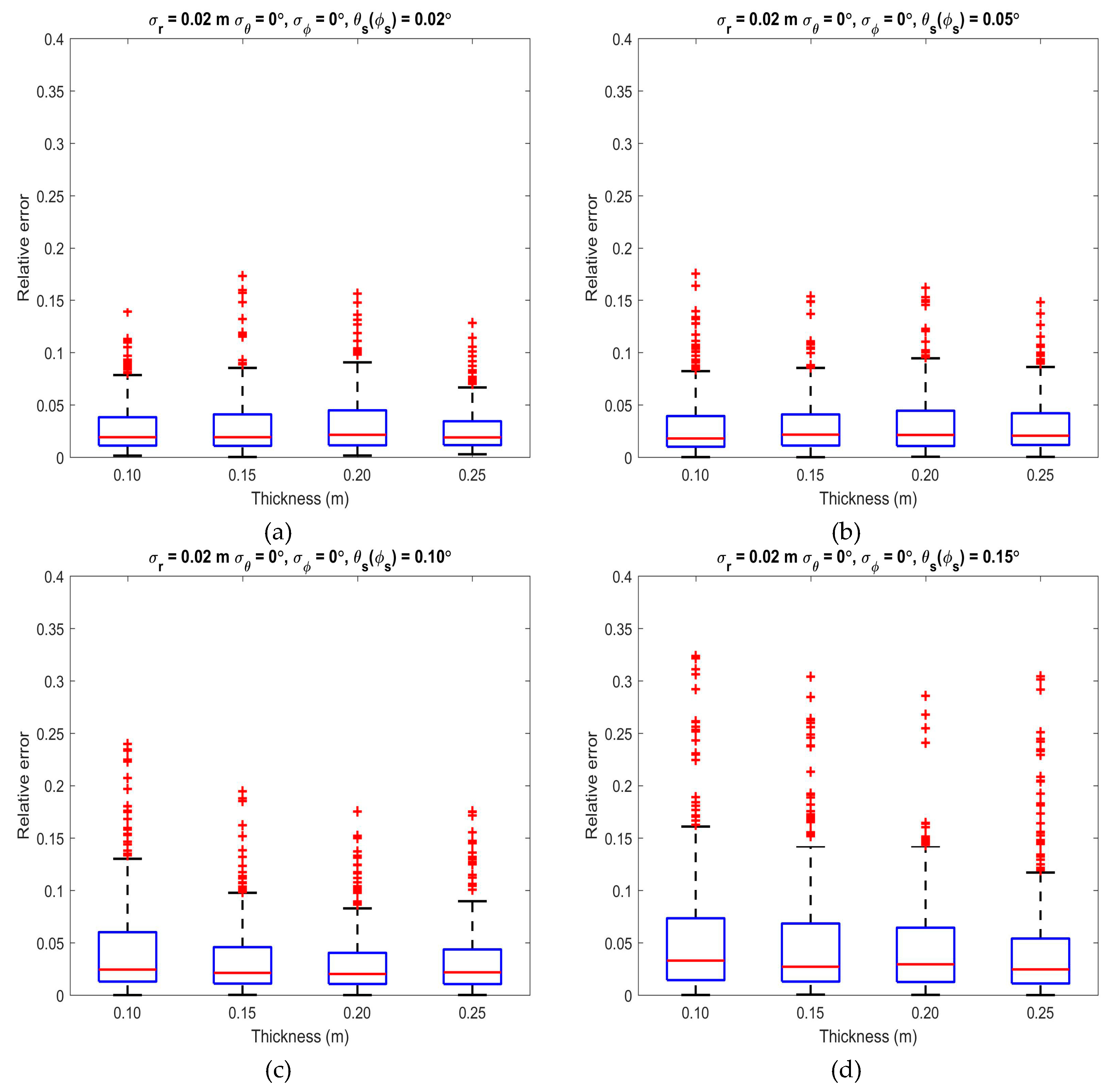
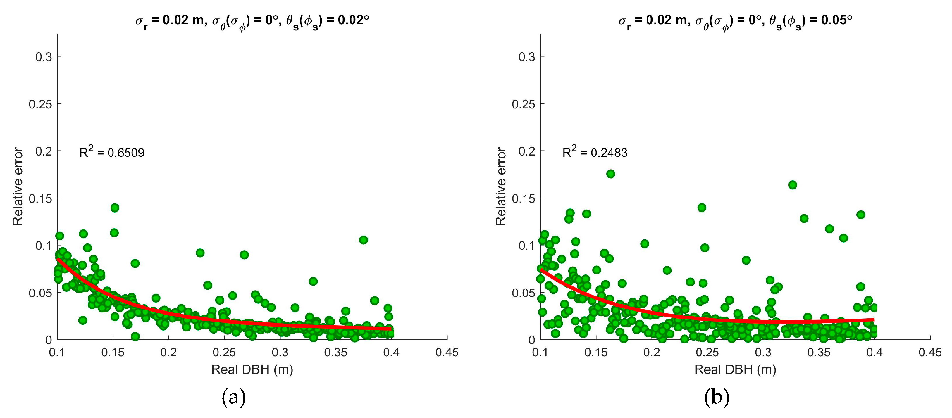
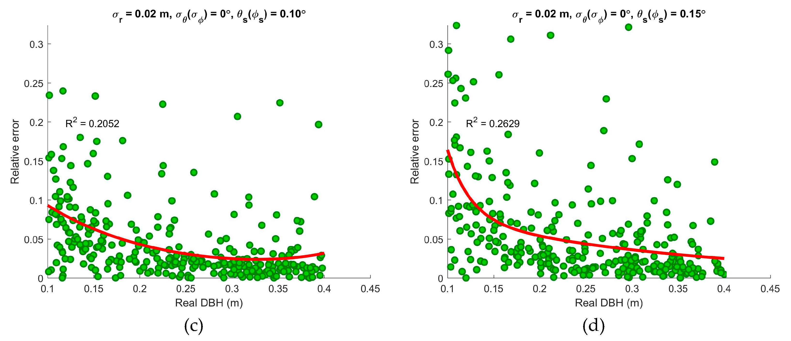
3.4. Impacts of the Slice Parameters

As previously described in the design of method, slice parameters included tree position, thickness and real DBH, which will be discussed in this part.
First, the tree position was described by using the distance. The impacts of the distance were determined by using group one of the dataset. Keeping σ φ ( σ θ ) at 0 degrees and θ s ( φ s ) at 0.02 degrees, the value of σ r was set as 0.02 m, 0.05 m, 0.10 m, and 0.15 m in turn. No relationship between the relative error and distance was evident (Figure 10). However, the relative errors were clearly relatively small when σ r was 0.02 m. No evident change was observed when σ r was set as 0.05 m, 0.10 m, and 0.15 m.
Second, the impacts of slice thickness on the relative error of the DBH estimation were illustrated by using group six of the dataset (Figure 11). Keeping σ r at 0.02 m and σ φ ( σ θ ) at 0 degrees, the value of θ s ( φ s ) was set as 0.02 degrees, 0.05 degrees, 0.10 degrees, and 0.15 degrees in turn, while the thicknesses of slices was set as 0.10 m, 0.15 m, 0.20 m and 0.25 m in turn. Four values of thickness were used to perform the simulation. No apparent change was shown when θ s and φ s were set as 0.02 ° and 0.05 ° . However, the relative error slightly decreased with increasing thickness when θ s and φ s set as 0.10 ° and 0.15 ° (Figure 11).
Third, the impacts of the real DBH on the relative error of the DBH estimation were illustrated by using group five of the dataset (Figure 12). Keeping σ r at 0.02 m and σ φ ( σ θ ) at 0 degrees, the value of θ s ( φ s ) was set as 0.02 degrees, 0.05 degrees, 0.10 degrees, and 0.15 degrees in turn. Unlike the distance, the real DBH shows a correlation with the relative error. A strong correlation was observed when the σ r was 0.02 m. Under each value of σ r , a similar trend was seen in which increasing the real DBH values decreased the relative errors.
Since the number of points in a slice and the scanning angular width were related to the slice parameters, they were also analyzed in this section by using group five of the dataset. Keeping σ r at 0.02 m and σ φ ( σ θ ) at 0 degrees, the value of θ s ( φ s ) was set as 0.02 degrees, 0.05 degrees, 0.10 degrees, and 0.15 degrees in turn.
As shown in Figure 13, the increasing number of points decreased the relative error, and the R-squared values mostly increased with increasing θ s and φ s (Figure 11).
Similar trends can be seen in Figure 14: the increasing scanning angular width decreased the relative error, and the R-squared values mostly increased with increasing θ s and φ s (Figure 11). Furthermore, a relatively strong relationship was observed between the scanning angular width and the relative error.

4. Discussion

In this paper, a simulator was constructed to study the impacts of three sets of parameters and two circle fitting methods. However, it must be emphasized that all the descriptions in the experiment were based on statistically simulated datasets, which were generated with the assumptions mentioned in the methods section. These descriptions are qualitative and not specific to certain TLS instruments.

4.1. Circle Fitting Methods

According to the simulation and estimation results (Figure 4), the estimation results of the two selected methods were good when the TLS instruments have a small range error, for example 0.02 m, which is very easy to reach for many commercial TLS instruments, such as the RIEGL VZ-400 scanner and FARO Photo 120 scanner. The range accuracy of RIEGL VZ-400 scanner was reported to be 5 mm at a 100 m distance. The maximum error in the distance of FARO Photo 120 scanner was reported to be ± 2 mm at a 25 m distance.
That is, the DBH estimation was not sensitive to the circle fitting method when the TLS instruments scanned with a high range accuracy. This is consistent with the conclusion of a previous paper [21], in which the performances of three circle fitting methods were evaluated by using the FARO Photo 120 scanner.
However, the impacts of the circle fitting method should be considered for a scanner whose range error is relatively large, such as SICK LMS511, whose systematic error is reported to be ± 35 mm at a distance of 10 m to 20 m and ± 50 mm at a distance of 20 m to 30 m [32]. The underestimated results of the two methods still have relatively good linearity and could be adjusted easily if the σ r of the scanner was not too large. When the value of σ r was close to the size of the DBH, the LM method was better than the Taubin method (Figure 4).
In terms of the estimation speed, the Taubin method was faster than the LM method, which included iterations (Figure 5). Therefore, the two circle fitting methods produced similar DBH estimations when the range accuracy was higher, while the Taubin method was less time consuming. The Taubin method may be a better choice for the scanning in which there is high range accuracy, which has advantages on the accuracy and speed simultaneously.

4.2. Error Parameters

Range error is a very important parameter for TLS instruments as well as for DBH estimation. The relative error of the DBH estimation was heavily affected by the range error (Figure 6 and Figure 9). A smaller range error was favorable for reducing the relative error. The reduction effect decreased with increasing range error.
Angular errors in vertical and horizontal directions demonstrated different performances on the accuracy of the DBH estimation. The angular error in the vertical direction showed little impact on the accuracy of the DBH estimation, while the angular error in the horizontal direction showed an evident impact (Figure 7 and Figure 8). Clearly, DBH estimation is based on the 2D projections of 3D point cloud data. In the process of reducing the dimensionality, the vertical distribution of points was eliminated, while the horizontal distribution of points directly affected the results of the circle fitting.
Based on the above analysis, it was easier to obtain an accurate DBH estimation with high range accuracy and high horizontal angular accuracy, which had major impacts on the accuracy of point distribution in the planar projection. Meanwhile, points with better accuracy and distribution were favorable for fast DBH estimation, especially for the geometrical circle fitting methods. Therefore, a TLS instrument with high range accuracy and high horizontal angular accuracy has an advantage in accurate and fast DBH estimation.
However, as the manufacturers of TLS instruments have claimed, range error and angular errors may vary with the distance between the scanner and the trunk slices. Forsman had reported that beamwidth is also an important parameter that affects the angular error and the accuracy of DBH estimation [18]. Therefore, error parameters are complicated in practice which should be studied further.

4.3. Scanning Parameters

Angular step widths in the horizontal and vertical directions are the parameters that can be changed in a field scan. As seen, they were not the dominant factors affecting the accuracy of the DBH estimation, especially with a larger σ r (Figure 9). However, they were important indicators of point cloud density. The smaller the angular step widths were, the greater the number of points that were acquired for a given slice. A finer angular step width required more scanning time, and high-density point cloud data created a storage and computation burden. As seen in Figure 9a, a similar accuracy of the DBH estimation was obtained when θ s and φ s were 0.02 ° or 0.05 ° , while the number of points differed by six times, which indicated that a suitable increase of angular step width may not improve the accuracy of DBH estimation significantly when high range accuracy was possible.

4.4. Slice Parameters

The slice parameters had comprehensive, although different, impacts on the accuracy of the DBH estimation with angular step widths.
It was determined that distance had a minor statistical impact on the relative error when different σ r values were used in the simulation (Figure 10). This conclusion was drawn based on the assumption that the σ r was stable with increasing distance. However, the σ r usually increased with increasing distance in practice, which caused the difference among the subfigures in Figure 10.
Our observations also showed that whether an increase in the thickness improved the accuracy of the DBH estimation depended on the angular step widths (Figure 11). The conclusion was drawn that increasing thickness increased the number of points, which slightly favored the accuracy of DBH estimation (Figure 13). However, this effect was not evident in the case of small angular step widths, in which the point density was already high enough (Figure 11a,b).
It is also well understood that relatively large values of the real DBH decreased the relative error of the DBH estimation (Figure 12). A larger DBH also means more points in the same situation. What needs special attention is that increasing thickness and increasing DBH can both increase the number of points. However, increasing thickness means increasing points in the vertical direction, and increasing DBH means increasing points in the horizontal direction. From another viewpoint, an increasing DBH also means that the slices are more likely to be detected more times by laser beams while increasing the scanning angular width. Compared with the thickness of a slice, the scanning angular width shows a stronger correlation with the accuracy of the DBH estimation (Figure 11 and Figure 14).
Besides the abovementioned factors, there are also some factors playing important roles on the DBH estimation in the field scanning, such as the terrain, the tilting of trees, the occlusion effect, etc. As the consequence of considering these factors, the DBH estimation will be more variable and complex.

5. Conclusions

The main goal of this study was to evaluate the impacts of error parameters, scanning parameters, trunk slice parameters, and circle fitting methods on DBH estimation. Based on a large number of the simulated trunk slices, these factors were discussed separately in the study.
As the research has demonstrated, the range error and the angular error in horizontal direction of the TLS instrument system played major roles in the accuracy of DBH estimation. The angular step width did not show much impact on accurate DBH estimation. However, the angular step widths determined the maximum amount of data, which is also affected by characteristics such as the tree position, slice thickness, and real DBH value. The algebraic circle fitting method and the geometrical circle fitting method have similar performances on the accuracy of DBH estimations when the range accuracy was higher, while the former has an advantage on computational efficiency. However, the geometrical circle fitting method has a better stability of DBH estimations while the range accuracy was lower.
Clearly, there is a need for further focus on the compound effect of these factors. More research should be performed to help design the field campaigns with specific TLS instruments to obtain accurate and fast DBH estimations.

Author Contributions

Conceptualization, P.W.; methodology, P.W., Q.Z.; software, P.W., G.B., X.G.; validation, P.W., X.G.; formal analysis, P.W., L.L.; data curation, P.W., X.X. (Xiuxian Xu); writing—original draft preparation, P.W., Y.L.; writing—review and editing, P.W., X.X. (Xiangming Xiao); visualization, P.W., Z.L.

Funding

This research is funded by the Fundamental Research Funds for the Central Universities (No. 2015ZCQ-LY-02) and the State Scholarship Fund from China Scholarship Council (CSC No. 201806515050).

Acknowledgments

Thanks to the editor and three anonymous reviewers for their insights and suggestions which helped us to improve the manuscript.

Conflicts of Interest

The authors declare no conflicts of interest.

References

  1. Pan, Y.; Birdsey, R.A.; Phillips, O.L.; Jackson, R.B. The Structure, Distribution, and Biomass of the World’s Forests. Annu. Rev. Ecol. Evol. Syst. 2013, 44, 593–622. [Google Scholar] [CrossRef]
  2. Maas, H.-G.; Bienert, A.; Scheller, S.; Keane, E. Automatic forest inventory parameter determination from terrestrial laser scanner data. Int. J. Remote Sens. 2008, 29, 1579–1593. [Google Scholar] [CrossRef]
  3. Telenius, B.F. A software tool for standardised non-destructive biomass estimation in short rotation forestry. Bioresour. Technol. 1997, 60, 267–268. [Google Scholar] [CrossRef]
  4. Liang, X.; Litkey, P.; Hyyppa, J.; Kaartinen, H.; Vastaranta, M.; Holopainen, M. Automatic Stem Mapping Using Single-Scan Terrestrial Laser Scanning. IEEE Trans. Geosci. Remote Sens. 2012, 50, 661–670. [Google Scholar] [CrossRef]
  5. Lovell, J.L.; Jupp, D.L.B.; Newnham, G.J.; Culvenor, D.S. Measuring tree stem diameters using intensity profiles from ground-based scanning lidar from a fixed viewpoint. ISPRS J. Photogramm. Remote Sens. 2011, 66, 46–55. [Google Scholar] [CrossRef]
  6. Strahler, A.H.; Jupp, D.L.B.; Woodcock, C.E.; Schaaf, C.B.; Yao, T.; Zhao, F.; Yang, X.; Lovell, J.; Culvenor, D.; Newnham, G.; et al. Retrieval of forest structural parameters using a ground-based lidar instrument (Echidna®). Can. J. Remote Sens. 2008, 34, S426–S440. [Google Scholar] [CrossRef]
  7. Yao, T.; Yang, X.; Zhao, F.; Wang, Z.; Zhang, Q.; Jupp, D.; Lovell, J.; Culvenor, D.; Newnham, G.; Ni-Meister, W.; et al. Measuring forest structure and biomass in New England forest stands using Echidna ground-based lidar. Remote Sens. Environ. 2011, 115, 2965–2974. [Google Scholar] [CrossRef]
  8. Hopkinson, C.; Chasmer, L.; Young-Pow, C.; Treitz, P. Assessing forest metrics with a ground-based scanning lidar. Can. J. For. Res. 2004, 34, 573–583. [Google Scholar] [CrossRef]
  9. Olofsson, K.; Holmgren, J.; Olsson, H. Tree Stem and Height Measurements using Terrestrial Laser Scanning and the RANSAC Algorithm. Remote Sens. 2014, 6, 4323–4344. [Google Scholar] [CrossRef]
  10. Calders, K.; Newnham, G.; Burt, A.; Murphy, S.; Raumonen, P.; Herold, M.; Culvenor, D.; Avitabile, V.; Disney, M.; Armston, J.; et al. Nondestructive estimates of above-ground biomass using terrestrial laser scanning. Methods Ecol. Evol. 2015, 6, 198–208. [Google Scholar] [CrossRef]
  11. De Tanago, J.G.; Lau, A.; Bartholomeus, H.; Herold, M.; Avitabile, V.; Raumonen, P.; Martius, C.; Goodman, R.C.; Disney, M.; Manuri, S.; et al. Estimation of above-ground biomass of large tropical trees with terrestrial LiDAR. Methods Ecol. Evol. 2018, 9, 223–234. [Google Scholar] [CrossRef]
  12. Hansen, E.; Gobakken, T.; Bollandsås, O.; Zahabu, E.; Næsset, E. Modeling Aboveground Biomass in Dense Tropical Submontane Rainforest Using Airborne Laser Scanner Data. Remote Sens. 2015, 7, 788–807. [Google Scholar] [CrossRef]
  13. Kankare, V.; Holopainen, M.; Vastaranta, M.; Puttonen, E.; Yu, X.; Hyyppä, J.; Vaaja, M.; Hyyppä, H.; Alho, P. Individual tree biomass estimation using terrestrial laser scanning. ISPRS J. Photogramm. Remote Sens. 2013, 75, 64–75. [Google Scholar] [CrossRef]
  14. Béland, M.; Widlowski, J.-L.; Fournier, R.A.; Côté, J.-F.; Verstraete, M.M. Estimating leaf area distribution in savanna trees from terrestrial LiDAR measurements. Agric. For. Meteorol. 2011, 151, 1252–1266. [Google Scholar] [CrossRef]
  15. Zheng, G.; Moskal, L.M. Leaf Orientation Retrieval From Terrestrial Laser Scanning (TLS) Data. IEEE Trans. Geosci. Remote Sens. 2012, 50, 3970–3979. [Google Scholar] [CrossRef]
  16. Pesci, A.; Teza, G.; Bonali, E. Terrestrial Laser Scanner Resolution: Numerical Simulations and Experiments on Spatial Sampling Optimization. Remote Sens. 2011, 3, 167–184. [Google Scholar] [CrossRef]
  17. Bailey, B.N.; Ochoa, M.H. Semi-direct tree reconstruction using terrestrial LiDAR point cloud data. Remote Sens. Environ. 2018, 208, 133–144. [Google Scholar] [CrossRef]
  18. Forsman, M.; Börlin, N.; Olofsson, K.; Reese, H.; Holmgren, J. Bias of cylinder diameter estimation from ground-based laser scanners with different beam widths: A simulation study. ISPRS J. Photogramm. Remote Sens. 2018, 135, 84–92. [Google Scholar] [CrossRef]
  19. Kankare, V.; Liang, X.; Vastaranta, M.; Yu, X.; Holopainen, M.; Hyyppä, J. Diameter distribution estimation with laser scanning based multisource single tree inventory. ISPRS J. Photogramm. Remote Sens. 2015, 108, 161–171. [Google Scholar] [CrossRef]
  20. Liang, X.; Hyyppä, J.; Kaartinen, H.; Lehtomäki, M.; Pyörälä, J.; Pfeifer, N.; Holopainen, M.; Brolly, G.; Francesco, P.; Hackenberg, J.; et al. International benchmarking of terrestrial laser scanning approaches for forest inventories. ISPRS J. Photogramm. Remote Sens. 2018, 144, 137–179. [Google Scholar] [CrossRef]
  21. Pueschel, P.; Newnham, G.; Rock, G.; Udelhoven, T.; Werner, W.; Hill, J. The influence of scan mode and circle fitting on tree stem detection, stem diameter and volume extraction from terrestrial laser scans. ISPRS J. Photogramm. Remote Sens. 2013, 77, 44–56. [Google Scholar] [CrossRef]
  22. Pueschel, P. The influence of scanner parameters on the extraction of tree metrics from FARO Photon 120 terrestrial laser scans. ISPRS J. Photogramm. Remote Sens. 2013, 78, 58–68. [Google Scholar] [CrossRef]
  23. Bu, G.; Wang, P. Adaptive circle-ellipse fitting method for estimating tree diameter based on single terrestrial laser scanning. J. Appl. Remote Sens. 2016, 10, 026040. [Google Scholar] [CrossRef]
  24. Liang, X.; Kankare, V.; Hyyppä, J.; Wang, Y.; Kukko, A.; Haggrén, H.; Yu, X.; Kaartinen, H.; Jaakkola, A.; Guan, F.; et al. Terrestrial laser scanning in forest inventories. ISPRS J. Photogramm. Remote Sens. 2016, 115, 63–77. [Google Scholar] [CrossRef]
  25. Watt, P.J.; Donoghue, D.N.M. Measuring forest structure with terrestrial laser scanning. Int. J. Remote Sens. 2005, 26, 1437–1446. [Google Scholar] [CrossRef]
  26. Kelbe, D.; Romanczyk, P.; van Aardt, J.; Cawse-Nicholson, K. Reconstruction of 3D Tree Stem Models from Low-Cost Terrestrial Laser Scanner Data; SPIE Defense, Security, and Sensing; Rochester Institute of Technology: Baltimore, MD, USA, 2013; p. 873106. [Google Scholar]
  27. Liang, X.; Kukko, A.; Kaartinen, H.; Hyyppä, J.; Yu, X.; Jaakkola, A.; Wang, Y. Possibilities of a Personal Laser Scanning System for Forest Mapping and Ecosystem Services. Sensors 2014, 14, 1228–1248. [Google Scholar] [CrossRef]
  28. Wang, P.; Li, R.; Bu, G.; Zhao, R. Automated low-cost terrestrial laser scanner for measuring diameters at breast height and heights of plantation trees. PLoS ONE 2019, 14, e0209888. [Google Scholar] [CrossRef]
  29. Chernov, N. Circular and Linear Regression: Fitting Circles and Lines by Least Squares; Taylor & Francis: Boca Raton, FL, USA, 2010; ISBN 978-0-429-15141-5. [Google Scholar]
  30. Lichti, D.D.; Jamtsho, S. Angular resolution of terrestrial laser scanners. Photogramm. Rec. 2006, 21, 141–160. [Google Scholar] [CrossRef]
  31. Lichti, D.D. A review of geometric models and self-calibration methods for terrestrial laser scanners. Bol. Ciênc. Geod. 2010, 16, 17. [Google Scholar]
  32. Product_Information_LMS5xx_Laser_Measurement_Technology_En_IM0038166.PDF. Available online: https://cdn.sick.com/media/docs/6/66/166/Product_information_LMS5xx_Laser_Measurement_Technology_en_IM0038166.PDF (accessed on 8 October 2019).
Figure 1. Flowchart of the method.
Remotesensing 11 02707 g001
Figure 2. The scanning geometry of a trunk slice.
Remotesensing 11 02707 g002
Figure 3. Illustration of two simulated slices. (a) Slice point cloud without errors. (b) Slice point cloud with the range and angular errors.
Remotesensing 11 02707 g003
Figure 4. Estimated results of the Levenberg–Marquardt (LM) method and the Taubin method when the angular errors in the vertical and horizontal directions were 0 degrees, and the angular step widths in the vertical and horizontal directions were 0.02 degrees. The results are shown when the range error was (a) 0.02 m, (b) 0.05 m, (c) 0.10 m and (d) 0.15 m.
Remotesensing 11 02707 g004
Figure 5. Time cost of the LM method and Taubin method when the angular errors in the vertical and horizontal directions were 0 degrees, and the angular step widths in the vertical and horizontal directions were 0.02 degrees. The results are shown when the range error was (a) 0.02 m, (b) 0.05 m, (c) 0.10 m and (d) 0.15 m.
Remotesensing 11 02707 g005
Figure 6. Illustration of the impacts of the range error on the relative error of the DBH estimation when the angular errors in the vertical and horizontal directions were 0 degrees, and the range error was set as 0.02 m, 0.05 m, 0.10 m, and 0.15 m in turn. The results are shown when the angular step widths in the vertical and horizontal directions were (a) 0.02 degrees, (b) 0.05 degrees, (c) 0.10 degrees and (d) 0.15 degrees.
Remotesensing 11 02707 g006
Figure 7. Illustration of the impacts of the vertical angular error on the relative error of the DBH estimation when the range error was 0 m, the angular error in the horizontal direction was 0 degrees, the angular step widths in the vertical and horizontal directions were 0.10 degrees, and the angular error in the vertical direction was set as 0.02 degrees, 0.05 degrees, 0.10 degrees, and 0.15 degrees in turn. (a) Plot on regular scale. (b) Regional magnification of plot (a).
Remotesensing 11 02707 g007
Figure 8. Illustration of the impacts of the horizontal angular error on the relative error of the DBH estimation when the range error was 0 m, the angular error in the vertical direction was 0 degrees, and the angular error in the horizontal direction was set as 0.02 degrees, 0.05 degrees, 0.10 degrees, and 0.15 degrees in turn. The results are shown when the angular step widths in the vertical and horizontal directions were (a) 0.02 degrees, (b) 0.05 degrees, (c) 0.10 degrees and (d) 0.15 degrees.
Remotesensing 11 02707 g008
Figure 9. Illustration of the impacts of the angular step widths on the relative error of the DBH estimation when the angular errors in the vertical and horizontal directions were 0 degrees, and the angular step widths in the vertical and horizontal directions were set as 0.02 degrees, 0.05 degrees, 0.10 degrees, and 0.15 degrees in turn. The results are shown when the range error was (a) 0.02 m, (b) 0.05 m, (c) 0.08 m and (d) 0.16 m.
Remotesensing 11 02707 g009
Figure 10. Illustration of the impacts of distance on the relative error of the DBH estimation when the angular errors in the vertical and horizontal directions were 0 degrees, and the angular step widths in the vertical and horizontal directions were 0.02 degrees. The results are shown when the range error was (a) 0.02 m, (b) 0.05 m, (c) 0.10 m and (d) 0.15 m.
Remotesensing 11 02707 g010
Figure 11. Illustration of the impacts of thickness on the relative error of the DBH estimation when the range error was 0.02 m, the angular error in the vertical and horizontal directions were 0 degrees. The results are shown when the angular step widths in the vertical and horizontal directions were (a) 0.02 degrees, (b) 0.05 degrees, (c) 0.10 degrees and (d) 0.15 degrees.
Remotesensing 11 02707 g011
Figure 12. Illustration of the impacts of the real DBH on the relative error of the DBH estimation when the range error was 0.02 m, the angular error in the vertical and horizontal directions were 0 degrees. The results are shown when the angular step widths in the vertical and horizontal directions were (a) 0.02 degrees, (b) 0.05 degrees, (c) 0.10 degrees and (d) 0.15 degrees.
Remotesensing 11 02707 g012aRemotesensing 11 02707 g012b
Figure 13. Illustration of the relationship between the number of points and the relative error of the DBH estimation when the range error was 0.02 m, the angular error in the vertical and horizontal directions were 0 degrees. The results are shown when the angular step widths in the vertical and horizontal directions were (a) 0.02 degrees, (b) 0.05 degrees, (c) 0.10 degrees and (d) 0.15 degrees.
Remotesensing 11 02707 g013
Figure 14. Illustration of the relationship between the scanning angular width and the relative error of the DBH estimation when the range error was 0.02 m, the angular error in the vertical and horizontal directions were 0 degrees. The results are shown when the angular step widths in the vertical and horizontal directions were (a) 0.02 degrees, (b) 0.05 degrees, (c) 0.10 degrees and (d) 0.15 degrees.
Remotesensing 11 02707 g014
Table 1. List of parameters and their purposes for simulated point cloud data.
Group No. σ r   ( m ) σ θ   ( deg ) σ φ   ( deg ) θ s & φ s   ( deg ) Purposes
10.02, 0.05, 0.10, 0.15000.02Circle fitting methods, distance
20.02, 0.05, 0.10, 0.15000.02, 0.05, 0.10, 0.15Range error, angular step width
300.02, 0.05, 0.10, 0.1500.10Vertical angular errors
4000.02, 0.05, 0.10, 0.150.02, 0.05, 0.10, 0.15Horizontal angular errors
50.02000.02, 0.05, 0.10, 0.15Number of points, real diameters at breast height (DBH), scanning angular width
60.02000.02, 0.05, 0.10, 0.15Thickness

