Article

Improving Forest Aboveground Biomass Estimation of Pinus densata Forest in Yunnan of Southwest China by Spatial Regression using Landsat 8 Images

1
Key Laboratory of State Forestry Administration on Biodiversity Conservation in Southwest China, Southwest Forestry University, Kunming 650224, China
2
Department of Geography, Southern Illinois University Carbondale, Carbondale, IL 62901, USA
*
Author to whom correspondence should be addressed.
Remote Sens. 2019, 11(23), 2750; https://doi.org/10.3390/rs11232750
Submission received: 21 October 2019 / Revised: 17 November 2019 / Accepted: 20 November 2019 / Published: 22 November 2019

Abstract

:
Uncertainties in forest aboveground biomass (AGB) estimates resulting from over- and underestimations using remote sensing data have been widely studied. The uncertainties may occur due to the spatial effects of the plot data. In this study, we collected AGB data from a total of 147 Pinus densata forest sample plots in Yunnan of southwestern China and analyzed the spatial effects on the estimation of AGB. An ordinary least squares (OLS) and four spatial regression methods were compared for the estimation using Landsat 8-OLI images. Through the spatial analysis of AGB and residuals of model predictions, it was found that the spatial autocorrelation and heterogeneity of the plot data could not be ignored. Compared with the OLS, the impact of the spatial effects on AGB estimation could be reduced slightly by the spatial lag model (SLM) and the spatial error model (SEM) and greatly reduced by the linear mixed effects model (LMM) and geographically weighted regression (GWR) based on the distributions of prediction residuals, global Moran’s I, and Z score. The spatial regression models had better performance for model fitting and prediction because of the reduction in overestimations and underestimations for the forests with small and large AGB values, respectively. However, the reductions in the overestimations and underestimations varied depending on the spatial regression models. The GWR provided the most accurate predictions with the largest R2 (0.665), the smallest root mean square error (34.507), and mean relative error (−9.070%) by greatly reducing the AGB interval for overestimations occurring and significantly increasing the threshold of AGB from 150 Mg/ha to 200 Mg/ha for underestimations. Thus, GWR offered the greatest potential of improving the estimation of Pinus densata forest AGB in Yunnan of southwestern China.

Graphical Abstract

1. Introduction

Trees grow by absorbing and using light, water, nutrients, and carbon dioxide, leading to accumulation of forest biomass. Thus, through carbon sequestration, forest biomass plays an important role in forest ecosystems and carbon cycling. Accurately estimating forest biomass is the basis of analyzing and understanding forest carbon dynamics and carbon cycling [1,2,3,4,5,6] and has been widely considered [7,8,9]. Obtaining total biomass of forests by field survey, including aboveground and belowground biomass, is very difficult and costly [1,2,3,5,6,10,11,12,13]. Because forest aboveground biomass (AGB) accounts for 70% to 90% of total forest biomass, most of the previous biomass studies focus on AGB [4,7,10,14,15].
Due to the availability of spatial information and large and repeated coverage, various remotely sensed data are often combined with field data from sample plots for estimating, mapping, and monitoring forest AGB at large scales [7,16,17]. Because of the lower cost, optical images from the Landsat and Sentinel satellites have been most widely used for these purposes. However, saturation of spectral reflectance from highly dense and multi-layer canopy forests leads to underestimations of forest AGB, and mixtures of spectral reflectance from soil and vegetation result in overestimations of AGB for young forests. Radar and LiDAR data that characterize tree heights and forest canopy structures, to some extent, mitigate the effects of the data saturation and mixture of spectral reflectance from soil and vegetation [9,13,16,17,18,19,20]. However, the high cost limits their applications to large areas. In addition, compared with the analysis of optical images, processing radar data is often more complicated and computation intensive. Some authors have studied the use of combinations of different data sources but developing appropriate data fusion algorithms remains challenging [9,13,16,17,18,19,20]. Thus, using optical images is still a good alternative for mapping forest AGB for large areas. Reducing the uncertainties due to the fact of overestimations and underestimations are still a challenge.
Various estimation methods, including parametric and non-parametric algorithms and machine learning methods, have been developed to reduce uncertainties in estimating forest AGB and to improve estimation accuracy using optical imagery based on strong correlations between spectral variables from the images and forest AGB [9,16]. Existing studies show that the determination coefficients (R2) between estimated and observed AGB values obtained by parametric models are often smaller than 0.5 [7,21]. Compared with parametric methods, non-parametric or machine learning approaches can lead to higher estimation accuracy because of their strong ability for fitting data, but they have a limited effect on improving AGB estimation because they are sensitive to sample designs (i.e., sample size and representativeness) [7,14]. Therefore, reducing uncertainties in estimating forest AGB using remotely sensed data is a great challenge [9,16,17,21] which has been widely recognized with substantial research conducted already [16,22,23]. The uncertainties are mainly caused by underestimations occurring in dense and multi-layered canopy and high biomass forests and by overestimations occurring in low biomass forests. Based on existing studies, underestimations often occur when forest AGB reaches 100 to 150 Mg/ha [9,21,24,25,26], and overestimations usually exist when AGB is less than 40 Mg/ha [9,21].
The uncertainties may also be due to the fact of ignoring spatial effects represented by spatial autocorrelation and heterogeneity [27,28,29,30,31,32,33,34,35]. Existing studies have shown that forest AGB data are often characterized by spatial autocorrelation and heterogeneity. Discarding spatial autocorrelation and heterogeneity will lead to biases of AGB estimation [33,36,37,38,39].
Spatial autocorrelation is the most commonly used method to account for spatial structure and distribution, such as random, clustering, and dispersion, and can be quantified at global and local levels [34,36]. Global spatial autocorrelation mainly describes the overall spatial structure and distribution of forest AGB, and Moran’s I [40], Geary’s C [41], and Getis’ G [42] statistics are commonly used [32,33,37]. Local spatial autocorrelation can test whether there are similar or dissimilar observations in local scales or determine the specific locations of “hot spots”, “cold spots”, and “outliers” [43,44,45], and local indicators of spatial association (LISA) [43], Moran’s Ii [40], and Getis’s Gi [42] are utilized.
Spatial heterogeneity shows the uniqueness of each location relative to other locations [35,46,47,48,49]. In the area of forest AGB, it represents the spatial complexity, change of ecosystem characteristics, and spatial difference caused by the non-random distribution of forest vegetation [38,49,50,51,52,53,54,55,56]. The methods used to evaluate and measure the spatial heterogeneity vary depending on the features of the spatial data including random index, aggregated index, nearest distance, trend surface, spectrum analysis, variation function, fractal dimension, analysis of variance ratio, correlation analysis, variation function, etc. [57,58,59,60,61,62]. Spatial autocorrelation and spatial regression models can also be used to analyze the spatial heterogeneity, especially the local autocorrelation [40,41,42,43]. Spatial regressions, particularly geographically weighted regression (GWR) models, are the most commonly used method to analyze spatial heterogeneity [32,33,46,47].
Because incorporating spatial effect analysis into regression models has no requirement for independent data, spatial regression models have been widely applied to improve understanding of forest distributions and estimation accuracy of forest parameters [32,37,38,39,44,45,63,64,65,66,67]. Corresponding to quantifying spatial autocorrelation and heterogeneity, globally and locally spatial regressions are used [37,38,39,44,63,66,67,68,69,70,71,72]. Spatial lag model (SLM), spatial error model (SEM), and spatial Durbin model (SDM) are the three most commonly used global models [34,37,39,65,66,67], while GWR is the most frequently used local spatial regression model [38,39,64,69,70,71,72]. Moreover, a mixed-effects model, including fixed effects and random effects, is also a commonly used spatial regression model, considering spatial autocorrelation in variance and covariance structures of the model [32,39,67]. Some authors have also employed spatial regression models, especially GWR, for estimating forest AGB using remote sensing data, with the modification of GWR by incorporating altitude information [13,73]. But, the authors ignored spatial effect analysis of AGB from sample plot data and model residuals. It was also unclear how the spatial regression models reduced overestimations and underestimations that often occur in forests with small and large AGB values, respectively. In addition, there have been no reports that deal with the analysis of the characteristics of spatial regression models and the differences of their contributions in reducing overestimations and underestimations.
The objective of this study was to present a method to improve mapping AGB for Pinus densata forests located in Yunnan of Southwest China. Both the spatial autocorrelation and heterogeneity of Pinus densata forest AGB data were first analyzed. Four spatial models, including SLM, SEM, linear mixed-effects model (LMM), and GWR, were then compared to estimate the forest AGB using Landsat 8 OLI imagery. Ordinary least squares (OLS) was also selected for comparison as a non-spatial model. The performance of the model fitting and prediction and the spatial effects of the residuals were evaluated for the five models. This study answers the following questions: (1) Can the spatial effect analysis be ignored for forest AGB estimation based on remote sensing data? (2) Do spatial models greatly reduce over- and underestimations in predictions? and (3) What are the differences in the contributions of the different spatial models to the reduction of the over- and underestimations of the predictions?

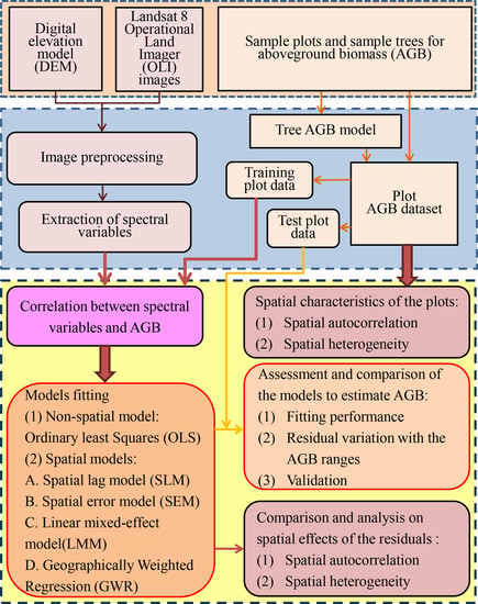
2. Materials and Methods

The methodological steps of this study are summarized in Figure 1. The methodological framework consisted of the following steps: (1) selection of the study area; (2) obtaining of the sample plot and tree AGB datasets; (3) acquisition and preprocessing of Landsat 8 OLI images and extraction of spectral variables; (4) correlation analysis of spectral variables with plot AGB, and selection of spectral variables; (5) spatial effect analysis of plot AGB; (6) development of one non-spatial and four spatial models; and (7) assessment and comparison of forest AGB estimation models, and the spatial effect analysis on the residuals of model predictions.

2.1. Study Area

In this study, the Pinus densata forests in Shangri-La City, northwest Yunnan Province, Southwest China were selected (Figure 2). The area is in the cold temperate zone with a monsoon climate. The altitude of Shangri-La City ranges from 1503 m to 5545 m above sea level. The high altitudes lead to sunny but chilly winters. This study area has an average annual temperature of 5.4 °C with the coldest and hottest months in December and July, respectively. There is an average annual precipitation of 607 mm with 70% of rainfall in June to September. The relative humidity is 70%, and the evaporation is 1671 mm. Dark brown forest soil and cold temperate coniferous forests are commonly found with dominant tree species of Abies, Pinus, Larix, and Picea [26].

2.2. Pinus Densata Forests

As a typical cool temperature coniferous tree species, Pinus densata forests are mainly distributed in sub-alpine and alpine areas with altitudes of 2800 m to 3700 m in the Hengduan Mountains. The Pinus densata forests of single tree species and canopy layer are common in this area. Even in the mixed forests, the dominant tree species often is Pinus densata with Picea likiangensis, Pinus armandii, Quercus pannosa, Betula spp. and Larix potaninii var. macrocarpa mixed [26,74].

2.3. Sample Plot Data and Forest Aboveground Biomass

A total of one hundred and forty-seven 30 m square sample plots were measured in 2016 (Figure 2). The plots were sampled with a distance of about 1 km based on the different stand ages, elevations, slopes, and aspects [26]. These factors were determined using a spatial distribution map of Pinus densata forests. In the map, forest compartments that had a homogeneous stand age, tree species composition, and canopy structures, elevations, slopes, and aspects were generated in the field using aerial photographs by visual interpretation. Within each plot, the plot coordinates, elevation, slope, and aspect were obtained. The tree variables including tree species, diameter at breast height (1.3 m) (DBH), and height (H) were measured and used to calculate tree biomass.
Because there were no tree biomass models available for Pinus densata forests, in this study, a sample tree was selected from each of the sample plots based on its average DBH and H. In order to reduce the cost, the selection of the sample trees was discarded for the sample plots that had similar characteristics of stand parameters. Thus, a total of 100 sample trees were obtained. Each sample tree was cut and the wood, bark, branches, needle biomass, H, and DBH were measured. The 3 cm thick disks were taken at a 2 m interval along each trunk and the volume was calculated. The disks were dried by oven to a constant weight at 105 °C and weighted. The sample density was obtained using a drainage method. At the same time, the volumes of wood and bark for each sample tree were calculated using 2 m segments and diameters without bark in every segment and then converted to biomass based on the sample density. Sample branches were graded and collected to weight the leaves and branches. A similar method was used to dry the branch and leaf samples. The biomass values of branches and leaves were yielded using the fresh weight and dry matter ratio. Summing the biomass values of woods, barks, branches, and leaves led to the total biomass of each sample tree. The power function was used to fit individual tree AGB data, resulting in following equation of tree biomass.
AGB = 0.073·DBH1.739·H0.880
The model had an R2 value of 0.992 and a root mean square error (RMSE) value of 30.778 kg, and it was used to estimate the AGB value of each Pinus densata tree in each of the plots. Equation (2) was employed to obtain the AGB of every plot that was then transferred to the value per hectare. The plot data were randomly divided into a fitting dataset of 117 plots and a test dataset of 30 plots (Table 1). This division of the dataset was conducted mainly considering that, in this study, there were relatively complex topographic features and a relatively great coefficient of variation (52.5%) for the forest AGB. Using a large sample size for model fitting can offer an opportunity of providing accurate estimates of AGB. At the same time, the test dataset should not significantly differ statistically from the fitting dataset in terms of their sample means and standard deviation. In fact, the random division led to a relatively great difference of the average AGB values between the fitting dataset and test dataset, but their sample means and standard deviations were not significantly different statistically from each other based on the student t-test distribution and F test at the significance level of 0.05. Thus, the division of the dataset would not significantly affect the conclusions drawn from the fitting and test datasets.
A G B s t a n d = i = 1 n A G B i 900 · 10000 / 1000

2.4. Collection and Preprocessing of Landsat 8 Images

In the present study, three Landsat 8 OLI images were downloaded from the website of the United States Geological Survey, and their image IDs are LC81310412016005LGN00, LC18320402016012LGN00, and LC81320412016012LGN00. There was a Universal Transverse Mercator coordinate system with zone 47 north in the images [26]. The images were mosaicked into one image and clipped using the shape file of the study area (Figure 2). The dark object subtraction approach was used to conduct atmospheric calibration of the mosaicked image [75], and the C-correction approach was utilized to carry out topographic correction using digital elevation model data at a spatial resolution of 30 m × 30 m [76,77].
A total of 253 remote sensing variables were extracted by ARCGIS including 7 bands, 22 vegetation indices, and 224 textural measures. The bands consisted of Band1—coastal aerosol, band2—blue (BLU), band3—green (GRN), band4—red (RED), band5—near infrared (NIR), band6—shortwave infrared 1 (SWIR1), and band7—shortwave infrared 2 (SWIR2). The 22 vegetation indices were consistent with those in the study by Ou et al. [26], including normalized difference vegetation index (NDVI), simple ratio index (RVI), difference vegetation index (DVI), perpendicular vegetation index (PVI), two soil adjusted vegetation indices, brightness, greenness and temperature vegetation indices, atmospherically resistant vegetation index (ARVI), modified soil adjusted vegetation index (MSAVI), etc. In addition, a total of 224 grey-level co-occurrence matrix-based texture measures including mean, angular second moment, contrast, correlation, dissimilarity, entropy, homogeneity, and variance were derived using moving windows of 3 × 3, 5 × 5, 7 × 7 and 9 × 9 pixels, respectively. The objective of using the vegetation indices and texture measures was to capture the characteristics of the forest canopy structure and textures [26,78,79]. Pearson correlation analysis between the remote sensing variables and AGB were carried out using SPSS 18.0 for Windows, and the spectral variables with significant correlation (p ≤ 0.05) were selected to build the AGB estimation models [26,72].

2.5. Spatial Effect Analysis

In this study, both the plot AGB and the residuals of the model predictions were analyzed for spatial autocorrelation and heterogeneity.

2.5.1. Spatial Autocorrelation

The spatial autocorrelation was investigated using both global and Anselin local Moran coefficients [32,43,80]. In this study, Moran’s I was used to describe the global spatial autocorrelation for the plot AGB and the residuals of the model predictions (Equation (3)).
I = n i = 1 n j = 1 n w i j ( d ) ( x i x ¯ ) ( x j x ¯ ) i = 1 n j = 1 n w i j ( d ) i = 1 n ( x i x ¯ ) 2
where n is the number of the sample plots, xi is the observation value at the different location, x ¯ is the average value of the plot observation values, and w i j ( d ) is the weight based on the distance between plots i and j. The global test was visualized using a Moran scatter plot [64] in which the slope of the regression line corresponded to Moran’s I, and the significance of Moran’s I was tested by the Z value to determine if the spatial autocorrelation of the observations existed. The Z value was calculated as follows:
Z ( I ) = I E ( I ) V a r ( I )
An absolute Z score value smaller than 1.96 indicates that the spatial distribution of the plot AGB was random and otherwise, the null hypothesis: random distribution can be rejected where a positive or negative index value implies a tendency toward clustering and dispersion of the plot AGB values, respectively. Moreover, the Moran’s I with different bandwidths was used to make a line chart, and the spatial autocorrelation with the change of lag distance was investigated. Each observed plot should have at least one adjacent plot to ensure the analysis results are valid. In this study, the minimum adjacent distance among the plots was 74 m, the average distance was 1082 m, and the maximum distance was 6287 m. Therefore, the initial bandwidth was set to be 6000 m for the global autocorrelation analysis.
The Anselin local Moran’s Ii was used to show the local distributions and patterns of the plot AGB [39,81]. In this study, local indicators included spatial association (LISA) [43] and Moran scatter plot. The local Moran’s Ii was calculated as follows:
I i = ( x i x ¯ ) j w i j ( d ) ( x j x ¯ )
The Anselin local Moran’s Ii statistics are utilized to identify significant hot spots—clustering of high values (HH), cold spots—clustering of low values (LL), and spatial outliers—high values surrounded by low values (HL) and low values surrounded by high values (LH). The scatter graph of the Anselin local Moran’s Ii can also be created to visually show the spatial aggregation of the plot AGB observations. In this study, the bandwidth of Anselin local Moran’s Ii was determined according to the results of the global Moran’s I analysis with the different lag distances.

2.5.2. Spatial Heterogeneity

Intra-block variance ( S i n t r a ) was used to quantify the local spatial variability according to existing studies [32,82] and calculated as follows:
S i n t r a = 1 B g = 1 B 1 n g h = 1 n g ( e g h e g ¯ ) 2
where e g h is the hth observation value or residual of model predictions in the gth block, and e g ¯ is the mean of observations or model residuals in the gth block. The spatial variance is a function of block size. The S i n t r a increases as the size of the blocks increases [32,83,84]. This study evaluated S i n t r a of the AGB values and residuals from different biomass models at a range of block sizes (spatial scales), i.e., 0.5, 1, 1.5, 20, and 30 m. In this study, both the global Moran’s I and local Moran’s Ii were calculated using Rookcase [85], an Excel Visual Basic (VB) add-in for exploring the global and local spatial autocorrelation.

2.6. The AGB Estimation using Remote Sensing Data

In this study, a non-spatial model, OLS, and four spatial models, including SLM, SEM, LMM, and GWR, were used and compared to improve the AGB estimation of Pinus densata forests.

2.6.1. Ordinary Least Squares (OLS)

The relationship between y and X can be regressed using Equation (7).
y = X β + ε
where y is the vector of the observed response variable, X is a known model matrix including a column of 1 (for intercept) and p independent variables, β is a vector of unknown fixed-effects parameters, and ε is a vector of random error terms. The estimate of β is obtained by the least squares methods.

2.6.2. Spatial Lag Model (SLM)

The SLM is accomplished by including a spatial lag term of the dependent variable y into the OLS model [32] and shown as follows:
y = X β + ρ W y + ε
where W is a row-sum standardized weight matrix, Wy is a spatially lagged response variable, ρ is a spatial autocorrelation parameter, and ε is a vector of random error terms with a normal distribution.

2.6.3. Spatial Error Model (SEM)

The SEM is the combination of the OLS model and the spatial autoregressive model [32] and shown as follows:
y = X β + λ W ε + ξ
where W is a row-sum standardized weight matrix, W ε . is a spatially lagged error term, λ . is a spatial autocorrelation parameter, and ξ is a well-behaved error term with a normal distribution.

2.6.4. Linear Mixed-Effects Model (LMM)

The LMM is a special case of generalized linear models and can be expressed by Equation (10):
y = X β + Z γ + ε
where y, X, and β are defined in Equation (9), Z is a known design matrix, ε is a vector of unobserved random errors, and γ is a vector of unknown random-effects parameters. The region’s random effect was analyzed for LMM across six townships of the study area, including Geza, Luoji, Jiantang, Xiaozhongdian, Nixi, and Hutiaoxia, and where the sample plots were selected.

2.6.5. Geographically Weighted Regression (GWR)

Geographically weighted regression is an expansion of the global ordinary regression model incorporating the distance weights of the geographical information. If each observation in the dataset has a weight of unity, the GWR model is equivalent to the OLS model [32]. The underlying model for GWR is shown as follows:
y = β 0 ( u i ,   v i ) + k = 1 p β k ( u i ,   v i ) X k + ε
where { β 0 ( u i ,   v i ) , β 1 ( u i ,   v i ) , …, β p ( u i ,   v i ) } are the (p + 1) regression coefficients for the location (ui, vi) in the study area, and ε is the vector of the random error terms with the normal distribution. The estimation of the parameters is based on the geographic weight matrix (Wi). For a location i, Wi = f (di, h), where di is the distance vector between the location i and all neighbors, and h is the bandwidth. The commonly used weight functions f (di, h) include a fixed spatial kernel, such as a Gaussian distance decay kernel function, and an adaptive spatial kernel, such as a bi-square distance decay kernel [32,39,86,87,88].
In this study, four variables were selected for the linear models from the spectral variables with significant correlation with AGB of Pinus densata forest at the significance level of 0.05 by forward stepwise regression using SPSS 18.0 for Windows. The selected spectral variables included the correlation texture measure for band 1 using the window size 3 × 3 (CC3_1), the angular second moment texture measure for band 1 using the window size at 7 × 7 (SM7_1), the dissimilarity texture measure for band 1 using the window size at 7 × 7 (DI7_1), and the correlation texture measure for band 7 using the window size 7 × 7 (CC7_3). The OLS, SLM, and SEM models were fitted using GeoDa software [89,90]. The LMM and GWR were fitted using R software, and the bandwidth of the spatial regression models was determined by the result of global Moran’s I analysis of the plot AGB with the different lag distances.

2.7. Model Evaluation

The selected spectral variables were applied to all the models. The model fitting was evaluated by three statistics, including the R2, RMSE, and Akaike information criterion (AIC) [25]. Meanwhile, the error was analyzed to understand the AGB estimation performance on reducing under- and overestimations for the spatial models based on six AGB classes with a 40 Mg/ha interval, namely, <40, 40–80, 80–120, 120–160, 160-200, and >200 Mg/ha. Moreover, the models were validated using the test dataset by four measures, including mean error (ME), mean absolute relative error (MAE), mean relative error (MRE), and mean absolute relative error (MARE). In addition, the spatial autocorrelation and heterogeneity of the model residuals were analyzed to enhance understanding of the spatial effects of AGB using the methods in Section 2.5.

3. Results

3.1. Spatial Characteristics of Stand Aboveground Biomass

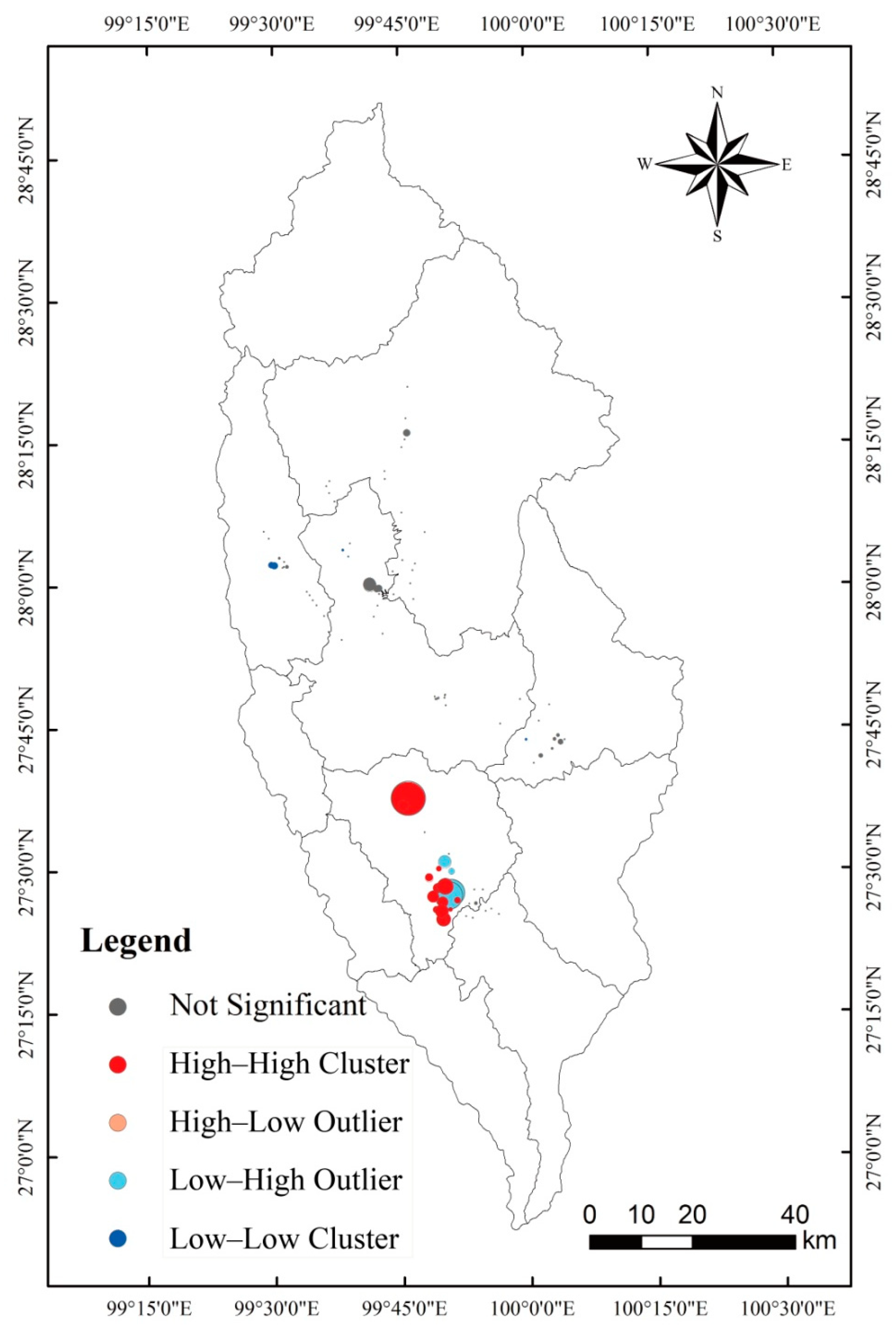
3.1.1. Spatial Autocorrelation

It was found that when the distance was 7.5 km, the global Moran’s I value was 0.1450 (Z score = 6.0228) (Figure 3), indicating a positive spatial autocorrelation at the lag distance and the spatial distribution of AGB clustering. The results of the local Moran’s Ii and the corresponding Z score of the AGB are listed in Table 2.
Moreover, the spatial distribution of the local Moran’s Ii values for AGB is shown in Figure 4, and the Z score values are listed in Table 3. Although 86.4% of the plot AGB values did not show significant spatial autocorrelation (|Z| < 1.96), 13.6% (that is, 20 plot AGB values) of 147 plot values were significantly spatially autocorrelated with each other. There were 17 (Z ≥ 1.96) plot values with significantly positive autocorrelation, out of which 13 plot values showed significantly High–High clustering and the other four plot values showed significantly Low–Low clustering (Z ≥ 2.58). In addition, there were three plot values with significantly negative autocorrelation (−2.58 < Z ≤ −1.96) and presenting Low–High outliers.

3.1.2. Spatial Heterogeneity

In Figure 5, intra-block variances with different block sizes for AGB were computed to reflect the spatial heterogeneity. The intra-block variances in AGB with lag distances represent the average local spatial variability for a given block size. The variances became larger as the block size increased before the distance of 30 km, then approached a stable level when the block size was relatively large with an approximately lag distance of 100 km.

3.2. Model Performance

The OLS model had an R2 = 0.239 and RMSE = 51.137 with statistically significant model coefficients (p < 0.05) except for the constant (Table 4). Four spatial regression models had greater R2 and smaller values of AIC and RMSE than OLS. According to a study by Fotheringham et al. [46], the difference between any two models is statistically significant if the AIC difference is greater than three. In this study, the OLS led to a greater AIC value than the four spatial models with the AIC difference between each of the four spatial models and the OLS being greater than three. Moreover, OLS had a smaller R2 value and a greater RMSE value than the four spatial models. Those indicated that the spatial regression models had significantly better performance for model fitting than OLS. The GWR had the greatest R2 (0.665) and the smallest values of AIC (1199.341) and RMSE (34.507), followed by LMM, SLM, SEM, and OLS based on the R2 values from high to low and the RMSE and AIC values from low to high. Thus, the GWR had the best performance for fitting, followed by LMM, SLM, SEM, and OLS.
Based on the test dataset (Table 4), the values for ME, MAE, MRE, and MARE of the five models showed a similar order of prediction performance as the AIC and RMSE obtained based on the model fitting dataset. The GWR had smaller values of ME, MAE, MRE, and MARE than LMM, SLM, SEM, and OLS. At the significance level of 0.10, the values of ME and MRE from GWR were significantly smaller than those from OLS, SEM, and SLM but not than those from LMM. Moreover, the significant difference of MAE only existed between GWR and OLS and between GWR and SLM, not between GWR and SEM, and between GWR and LMM. In addition, the value of MARE from GWR was significantly smaller than those from SLM and LMM but not than those from OLS and SEM.
Table 5 shows the estimates of the regression coefficients and the corresponding standard errors for the models OLS, SEM, SLM, and LMM and the mean regression coefficients and their ranges for GWR. For the four models, OLS, SEM, SLM, and LMM, the constant values differed from each other, but their standard errors were similar. For the same spectral variables, the values of the regression coefficients and their standard errors from OLS, SEM, SLM, and LMM were similar to each other, and the OLS had slightly larger absolute values of regression coefficients while LMM had slightly smaller absolute values of regression coefficients. Moreover, the average values of the regression coefficients from GWR were also similar to those of the other three spatial models, but the regression coefficients from GWR had wide ranges, indicating that the GWR model produced local spatial variability of the regression coefficients and, thus, forest AGB [32,67].
In Figure 6, the scatter graphs of the observed and predicted AGB values for the five models are shown to indicate the fitting performance. The GWR had the greatest value of R2, followed by LMM, SLM, OLS, and SEM. The overestimations and underestimations were obviously noticed for OLS, SEM, SLM, and LMM when the observed AGB was smaller than 70 Mg/ha and larger than 150 Mg/ha, respectively, and GWR greatly reduced the overestimations and underestimations by decreasing the interval of AGB values for the overestimations occurring and increasing the threshold greater than which the underestimations started to take place.
The maps of the predicted AGB values for Shangri-La City were generated using five models in Figure 7. The spatial distributions of the predicted AGB values looked similar to each other. But, by reducing the over- and underestimations, the map by GWR was more heterogeneous than those by OLS, SEM, SLM, and LMM.

3.3. Characteristics of Residuals with AGB Classes

In order to quantitatively compare the estimates using different models, the means and standard deviations of residuals from the model predictions of AGB were calculated for the overall and different AGB classes based on the test dataset. All the models led to similar trends in the residuals (Table 6). With the increase in AGB values, the means of the residuals changed from larger positive values (serious overestimations) to smaller positive values (slight overestimations), smaller negative values (slight underestimations), and large negative values (serious underestimations), while the standard deviations varied slightly. The overestimations and underestimations were the smallest for the AGB classes of 80 Mg/ha to 120 Mg/ha and 120 Mg/ha to 160 Mg/ha, and the largest for the AGBB classes of <40 Mg/ha and >200 Mg/ha, respectively, for all the models. The overestimations were obviously noticed when the AGB values were smaller than 80 Mg/ha, while the underestimations occurred when the AGB values were greater than 160 Mg/ha. For all models, the overall averages of the residuals were not significantly different from zero at the significance level of 0.05. Moreover, for the same class of AGB, GWR had the smallest absolute means of residuals for each of the AGB classes among the five models, although the overall average residual was the largest. The absolute means of the residuals from OLS, SEM, and SLM were not obviously different from each other, and, compared among these three models, LMM had a slightly smaller absolute mean.

3.4. Spatial Effect Analysis for the Models

The five models were assessed by examining the distributions of the residuals from the modeling dataset (Table 7). The OLS, SEM, SLM, and LMM had similar and large ranges of residuals. The OLS, SLM, and SEM produced positive skewness and negative kurtosis for their distributions of residuals with similar averages and standard deviations. Compared with OLS, SEM, and SLM, the LMM had a smaller standard deviation with negative skewness and kurtosis. The GWR yielded the smallest range and standard deviation of the residuals with a positive skewness and kurtosis.

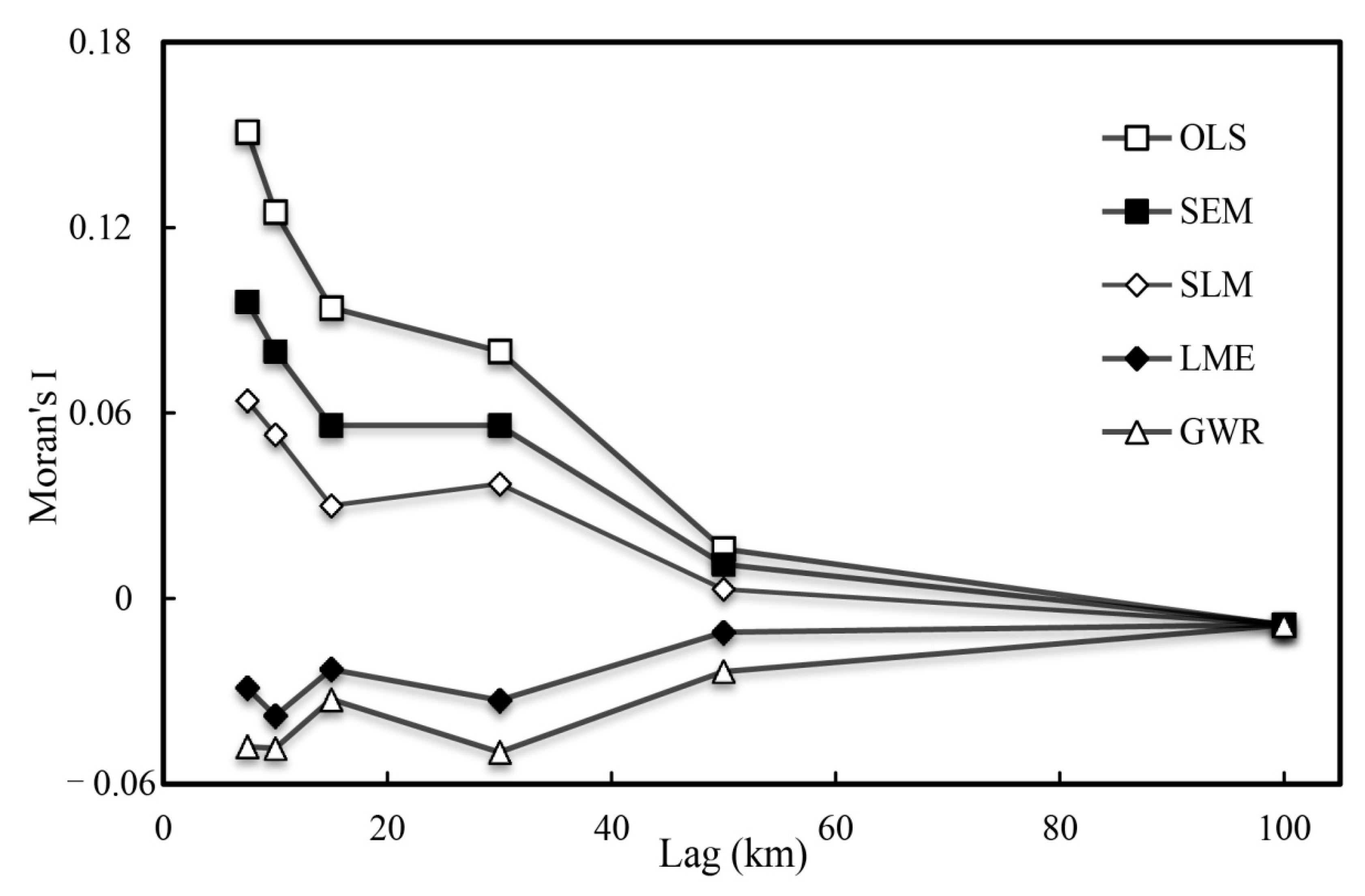
3.4.1. Spatial Autocorrelation of the Model Residuals

The global Moran’s I values of the five models with different lag distances are shown in Figure 8. Both OLS and SEM had larger absolute values of Moran’s I than SLM, LMM, and GWR. With the increase in lag distances, the absolute values of Moran’s I for all five models decreased, and the differences in the Moran’s I values among the models also decreased. The differences were not obvious when the lag distance reached 100 km.
The five models were fit at the bandwidth of 7.5 km. The global Moran’s I values and the corresponding Z scores for the residuals from OLS, SEM, SLM, LMM, and GWR are listed in Table 8. The Z scores were significantly positive (Z-values > 1.96) for OLS and SEM, indicating that the three models produced similar clustering patterns for the prediction residuals at a significance level of 0.05. The Z score for SLM is positive, and the values both GWR and LMM were negative, and their absolute values were smaller than 1.96.
The statistics for the local Moran’s Ii values of the prediction residuals for the five models are listed in Table 9. The local Moran’s Ii values of the models had negative skewness but positive kurtosis. The OLS, SLM, and SEM had similar averages, standard deviations, skewness, and kurtosis, and the means of the local Moran’s Ii values were positive and greater than the corresponding absolute values from LMM and GWR. The ranges in the local Moran’s Ii values from OLS, SLM, and SEM were also greater compared with those from the other two models. The LMM model yielded the smallest range, standard deviation, and absolute mean value of local Moran’s Ii. The GWR had a smaller standard deviation and the greatest absolute skewness and kurtosis values.
Figure 9 presents the local spatial autocorrelation characteristics of the prediction residuals based on the local Moran’s Ii values for the five models. For the prediction residuals of OLS, SEM, and SLM, the hot spots (high–high clustering) were found at the southwest central part of the study area, while the cold spots were noticed at the west central part with low–high outliers located at the southwest central part. The LMM only led to one hot spot, one cold spot, and one low–high outlier; the GWR resulted in one cold spot and a few outliers but no hot spots.
Table 10 lists the statistical parameters of the Z scores for the five models. Out of 117 sample plots, 98, 99, and 103 plots had no significant spatial autocorrelation of the model residuals with |Z| values smaller than 1.96 for OLS, SEM, and SLM, respectively; more than 110 plots for GWR and LMM did not show significantly spatial autocorrelation of the prediction residuals. Moreover, the number of plots with significant spatial autocorrelation of the residuals with |Z| ≥ 1.96 from OLS, SEM, SLM, LMM, and GWR were 19, 18, 14, 3, and 5, respectively. This implies that, compared with OLS, SEM and SLM, the spatial models LMM and GWR greatly reduced the spatial autocorrelation of the residuals.

3.4.2. Spatial Heterogeneity of the Model Residuals

The intra-block variances of the prediction residuals from the five models’ given block sizes are shown in Figure 10. All five models showed a similar trend of variance change, in that the variances became larger as the block size increased and approached a stable level when the block size was large enough. Moreover, the OLS, SLM, SEM, and LMM had similar and much larger intra-block variances of the residuals across all lag distances, and the stable variances were obtained when the block size was approximately 30 km. The variances of the residuals from GWR were the smallest at all lag distances, and the variances started to tend to stable when the block size was approximately 16 km.

4. Discussion

4.1. Spatial Effects

We investigated both the spatial autocorrelation and heterogeneity of AGB for Pinus densata forests from the sample plot data and found that the spatial effects should not be ignored when estimating the AGB using remote sensing images. The spatial autocorrelation occurred among the AGB plots because 13.61% of the plots were high–high or low–low clustering. But, there were fewer clustering points of the prediction residuals for the spatial regression models than OLS. Especially, LMM and GWR had more points which had no significant spatial autocorrelation, indicating that the spatial autocorrelation and the impact could be greatly reduced by the two spatial regression models. Moreover, the spatial heterogeneity could be found and the intra-block variances became larger as the block size increased. Although the spatial variability can also be decomposed into intra-block variance, inter-block variance, and total spatial variance [32,82,84], intra-block variance is often used to quantify the local spatial heterogeneity [32,82,84,91,92,93,94]. This study showed that four spatial regression models had smaller intra-block variances than OLS at the same lag distance. Especially, GWR greatly reduced the intra-block variances and improved the estimation of AGB compared with the other four models. This indicated that the spatial heterogeneity should not be ignored for the estimation of AGB using remote sensing images and that GWR could more effectively account for the spatial heterogeneity.
Moreover, it is of great importance for spatial effect analysis to select the proper bandwidths. The coefficient estimates of the spatial models may change and lead to different model performance [67]. In general, large and small bandwidths should be used for sparsely and densely distributed data, respectively [86,94,95,96]. In this study, we calculated the Global Moran’s I values and the corresponding Z-values of AGB plot data with lag distances from 6 km to 100 km. Overall, both the global Moran’s I and Z-values decreased gradually. The Z score values were greater than 1.96 when the distance was smaller than 76 km, and they were smaller than 1.96 after 76 km. Correspondingly, the positive Moran’s I values turned negative at a distance of 76 km. More importantly, as the distance increased, the Moran’s I values increased at the beginning and reached the first peak point with a value of 0.1450 (Z score = 6.0228) at the distance of 7.5 km, and the lag distance corresponding to the first peak point could be used as the bandwidth of the spatial regression models [36]. Therefore, the lag distance was selected for the spatial analysis and spatial regression, indicating the existence of significantly positive spatial autocorrelation and a clustering distribution for AGB of the plots.

4.2. Model comparison

This study showed that all the spatial regression models had better performance for model fitting and prediction for Pinus densata forest AGB compared with the non-spatial regression model OLS. This was mainly because there were significantly global and local spatial autocorrelations and spatial heterogeneities of AGB, and OLS lacked the ability to account for these spatial characteristics.
Among the spatial regression models, the performance of model fitting and prediction varied depending on the features of the landscape and models. In this study, GWR provided the greatest estimation accuracy (R2 = 0.665, RMSE = 34.507, MARE = 40.1%) of the forest AGB for both model fitting and test datasets, followed by LMM. Both SEM and SLM had similar and slightly better performances than OLS but poorer performances than GWR and LMM. The differences in the performances among the spatial regression models might result from the principles of the model development and the characteristics of the used data. The SLM is a formal representation of a spatial diffusion process which reflects the spatial dependence in the data and focuses on the assessment of the spatial dependence [32]. The SEM is developed based on the spatial autoregressive model with errors on the premise of no change for the explanatory variables [32,33], and it is assumed that the spatial autoregressive process occurs only in the error term, neither in the response variable nor in the predictor variables [64,97]. In short, although both the SEM and SLM models can explain the global spatial autocorrelation, they cannot deal with local spatial heterogeneity [33]. In fact, in this study, there was a global spatial autocorrelation of the AGB, but the spatial autocorrelation was only significant in a few portions of the study area. There were 86.39% of the plots and 83.76% of the prediction residuals from OLS in which the plot AGB and residual values were not significantly spatially autocorrelated with each other. On the other hand, in only 14% to 16% of the plots did significant spatial autocorrelation of AGB existed. Therefore, SLM and SEM might be selected to explain the spatial effect of the AGB plots. However, the improvement in the AGB estimation was limited.
The LMM had better performance than SEM and SLM and offered more accurate estimates of AGB by taking into account the effects of spatial autocorrelation with the spatial covariance structure and random effects incorporated [32,98]. The LMM can deal with both spatial autocorrelation and heterogeneity. However, the capacity for explaining spatial heterogeneity depends on random effects. In this study, the study area was considered to have random effects and LMM could, to some extent, account for the spatial heterogeneity, but it could not completely explain the spatial variation of the plot AGB. Moreover, LMM lacks the ability of accounting for the spatial variability due to the multiple random effects from environmental factors and forest heterogeneity. For this purpose, a good alternative is to use multi-level mixed-effects models. The GWR can not only accommodate spatial heterogeneity, but can also take into account spatial autocorrelation of AGB [39,46,72,95]. The results of prediction residuals from GWR showed that the spatial autocorrelation of the model residuals and the intra-block variances were greatly reduced compared with those from LMM, SLM, and SEM. This implied that GWR provided a powerful tool to potentially improve the estimation of AGB using remote sensing data. However, it has to be pointed out that all the models cannot explain in what way and how the estimation of AGB is affected by the factors.
The GWR led to the most accurate estimates of Pinus densata forest AGB in this study. This does not mean that it will certainly work better than other methods for all study areas. Chen et al. [15] found that support vector machine for regression performed better than GWR in the estimation of forest AGB in the center of the Changbai Mountains of China using sentinel imagery. This may be mainly due to the fact that the performance of the models often varies depending on the characteristics of the relationships between forest AGB and predictors and the ability of the models to model the relationships, sample sizes, and representative sample data for AGB populations. Non-parametric or machine learning models, such as artificial neural networks and support vector machine, may have stronger capacities to estimate forest AGB when there are complex non-linear relationships between predictors and forest AGB [9]. But almost all non-parametric methods are sensitive to the characteristics of sample data. When a sample size is small and its representativeness of the population is poor, non-parametric methods will have a weak predictive ability [9]. Non-parametric methods also lack the ability to offer a clear mathematical relationship, as the parametric models analyze the spatial effects. On the other hand, parametric methods, such as GWR, often have stronger predictive ability with clearer mathematical explanations than the non-parametric methods and are not as sensitive to the characteristics of the sample data for estimation of forest AGB. In addition, GWR often works better than most traditional non-spatial parametric models and global spatial regression models because of its strong ability for modeling spatial autocorrelation and spatially heterogeneous processes at local scales [53].

4.3. Overestimation and Underestimation

Over- and underestimations commonly exist in the estimation of forest AGB using remote sensing images. This study showed that the spatial effects of the plot AGB data that lead to overestimation and underestimation could not be ignored, and that the spatial regression models can improve the estimation accuracy of Pinus densata forest AGB. However, not all of the spatial regression models could significantly reduce the over- and underestimations. The major challenge for biomass estimation using optical imagery is the uncertainties from the underestimations in forests with high AGB and the overestimations in forests with low AGB [17,24,25,78]. Many studies have indicated that the uncertainties are relevant to forest ecosystems, topographic characteristics, remote sensing data, etc. [24,78,99,100,101,102,103,104]. In this study, SLM, SEM, and LMM had thresholds of overestimations and the underestimations similar to those of OLS, indicating that the three spatial regression models could not significantly reduce the uncertainties from the over- and underestimations. Compared with OLS, SEM, SLM, and LMM, the GWR significantly increased the estimation accuracy of Pinus densata forest AGB by lowering the threshold of overestimations and increasing the threshold of underestimations. Particularly, the overestimations from GWR in this study did not look obvious. The GWR is thus a powerful tool for reducing the uncertainties due to the overestimations and underestimations of forest AGB using remote sensing data and for increasing the estimation accuracy mainly because GWR takes into account both the spatial autocorrelation and spatial heterogeneity of AGB.

4.4. Comparison and Implication of Similar Studies

Several studies have been conducted to map AGB of Pinus densata forests in a similar area using Landsat images. In order to make a consistent comparison, the MARE values of the model predictions obtained based on the test datasets were mainly employed. Yue [105] compared a linear regression, artificial neural network, and support vector machine for regression with 147 sample plots measured in 2008 and Landsat images acquired in 2008 and 2009 to estimate Pinus densata forests AGB and obtained the MARE values of 26.36%, 23.31%, and 19.65%, respectively. Sun [106] estimated AGB of Pinus densata forests using a stepwise regression, a three-order polynomial regression, a system of equations, random forests, and Cubist with 57 sample plots and Landsat images obtained in 2014, and yielded MARE values of 51.3%, 48.2%, 51.7%, 15.4%, and 45.3%, respectively. Ou et al. [26] further explored the improvement of estimating Pinus densata forest AGB in this study area using a linear regression, a linear regression with combined variables, an artificial neural network, and random forests and produced the relative RMSE values of 45.5%, 48.5%, 38.5%, and 31.5%, respectively. By adding the age dummy variable into the models, the authors then reduced the corresponding relative RMSE values to 27.0%, 27.3%, 23.9%, and 21.5%. In this study, OLS, SEM, SLM, LMM, and GWR led to MARE values of 41.1%, 40.5%, 44.1%, 44.9%, and 40.1%, respectively. This implies that the results of this study were only compatible with those from the previous studies. However, the emphasis of this study was put on the consideration of spatial dependency and heterogeneity by GWR and, thus, on the reduction of overestimations and underestimations for forests with small and large values of AGB, respectively.
The results of all the relevant studies indicate that the accuracies of the model predictions vary greatly. The significant differences may be caused by the different datasets used, the different number of sample plots, the different quality of images, the different spectral variables, etc. First of all, the studies were conducted using different datasets collected from different times, and the forest canopy structures might have changed due to the natural factors such as diseases and insects as well as human activities such as clear-cutting. The studies used different sample sizes for model calibration and tests. Sun [106] employed field data collected in 2014 from a total of 56 sample plots with 39 plots for model fitting and 17 for model test and yielded the absolute values of the correlation coefficients between AGB and the used spectral variables ranging 0.324 to 0.468. In the study by Sun [106], overall, the obtained estimation accuracies were lower than those in this study except for random forest that led to a higher accuracy of 84.6%. However, the sample sizes used by Sun [106] for both model calibration and tests were too small. The small sample sizes might have led to significantly higher correlations of AGB with the spectral variables than those in the other studies of this area.
Yue [105] utilized a total of 147 sample plots with 101 plots for model fitting and 46 plots for model tests which were similar to those used in this study. However, the study by Yue [105] had significantly higher estimation accuracies than those in this study. The main reason might be because, in those models, the used spectral variables had greater absolute coefficients of correlation with AGB, ranging from 0.227 to 0.381, compared with the corresponding values from 0.200 to 0.326 in this study. The spectral variables with higher correlations in the study by Yue [105] included a shadow fraction derived by a spectral unmixing analysis and three skewness texture measures. The shadow fraction improved the estimation of AGB mainly because it characterized the impacts of shadows due to the large differences in the elevation and topographic complexity of the mountainous area. The skewness texture measures accounted for the feature of spatial distribution from the spectral reflectance values of Pinus densata forest canopy structures in this area. In this study, although two correlation texture measures, one angular second moment and one dissimilarity texture measure were selected to develop the models, the skewness texture measures and shadow fraction were not involved. This implies that the skewness texture measures and shadow fraction provide the potential to improve the estimation accuracy of Pinus densata forest AGB in this area and should be included in the estimation models to further increase the prediction accuracy in the future study.
Based on the relevant studies [26,105,106], it is commonly found that support vector machine and random forests provide the most accurate estimates of Pinus densata forest AGB. However, both methods theoretically are highly sensitive to sample size and representativeness [7,9] and require a large sample size which will lead to high cost. Both methods are also less generalizable and lack transferability for future use. Generalization and transferability will greatly enhance the application of the models. Moreover, adding the age as a dummy variable into the models showed the great potential for increasing the estimation accuracy of Pinus densata forest AGB [26]. However, the spatially explicit values of the forest stand age are usually not available which limits the application of the method. Overall, obtaining a high estimation accuracy of Pinus densata forest AGB in this area is very challenging mainly due to the fact of its complex landscape and topography and great differences in elevation. To further improve the estimation of Pinus densata forest AGB, attention should be paid to the selection of methods that can account for spatial dependency and spatial heterogeneity and which have strong capacity for prediction and transferability. At the same time, the emphasis should also be put on the selection of image texture measures and spatial features that can characterize the complexity of the landscape and topography in this area and the canopy structures of Pinus densata forests. Thus, it is expected the integration of GWR with the significantly correlated texture measures and shadow and vegetation fractions would offer greater potential for improving the estimation of Pinus densata forest AGB.

5. Conclusions

This research focused on improving the estimation of Pinus densata forest AGB using remote sensing images and spatial regression models. In this study, the spatial effects of Pinus densata forest AGB in the Yunnan Province of China was analyzed and quantified based on the fitting and test datasets from 117 and 30 sample plots, respectively, and Landsat 8-OLI images. As expected, GWR had the best performance with the largest R2 (0.665) and the smallest RMSE (34.507) and MARE (40.1%), followed by LMM, SLM, SEM, and OLS. More importantly, this study led to the following new conclusions: (1) spatial autocorrelation and spatial heterogeneity should not be ignored for AGB estimation using remote sensing data, and the impacts of spatial effect can be reduced by the spatial regressions; (2) given a forest landscape, the ability of the spatial regression models to reduce the uncertainties from over- and underestimations varies depending on the characteristics of the models; (3) the obtained AGB intervals smaller than 70 Mg/ha and larger than 150 Mg/ha for the over- and underestimations, respectively, were similar for SLM, SEM, and OLS. Compared with the other models, both LMM and GWR decreased the uncertainties from the over- and underestimations, but the decrease in the uncertainties was significant when using GWR and not when using LMM. Especially, GWR did not lead to overestimations and, at the same time, increased the threshold of the underestimations from 150 Mg/ha to 200 Mg/ha. Thus, the GWR method provides great potential for improving the estimation of forest AGB using Landsat 8 images.

Author Contributions

G.O. participated in field work, performed data analysis, and wrote the paper. Y.L. helped in the data analysis and wrote the paper. H.X. and G.W. supervised and coordinated the research, designed and installed the experiment, took some measurements, and contributed to the revision of the paper.

Funding

The study was financially supported by the National Natural Science Foundation of China (No. 31660202, 31760206, 31770677), the Expert Workstation of Yunnan Province (2018IC100), and the Ten-Thousand Talents Program of Yunnan Province (YNWR-QNBJ-2018-184).

Conflicts of Interest

The authors declare no competing financial interests.

References

  1. Houghton, R.A. Aboveground forest biomass and the global carbon balance. Glob. Chang. Biol. 2005, 11, 945–958. [Google Scholar] [CrossRef]
  2. Gibbs, H.K.; Brown, S.; Niles, J.O.; Foley, J.A. Monitoring and estimating tropical forest carbon stocks: Making REDD a reality. Environ. Res. Lett. 2007, 2, 4. [Google Scholar] [CrossRef]
  3. Keith, H.; Mackey, B.G.; Lindenmayer, D.B. Re-evaluation of forest biomass carbon stocks and lessons from the world’s most carbon-dense forests. Proc. Natl. Acad. Sci. USA 2009, 106, 11635–11640. [Google Scholar] [CrossRef] [PubMed]
  4. Pan, Y.; Birdsey, R.A.; Fang, J.; Houghton, R.; Kauppi, P.E.; Kurz, W.A.; Phillips, O.L.; Shvidenko, A.; Lewis, S.L.; Canadell, J.G.; et al. A large and persistent car bon sink in the world’s forests. Science 2011, 333, 988–993. [Google Scholar] [CrossRef] [PubMed]
  5. Schimel, D.; Pavlick, R.; Fisher, J.B.; Asner, G.P.; Saatchi, S.; Townsend, P.; Miller, C.; Frankenberg, C.; Hibbard, K.; Cox, P. Observing terrestrial ecosystems and the carbon cycle from space. Glob. Chang. Biol. 2015, 21, 1762–1776. [Google Scholar] [CrossRef] [PubMed]
  6. Goetz, S.J.; Hansen, M.; Houghton, R.A.; Walker, W.; Laporte, N.; Busch, J. Measurement and monitoring needs, capabilities and potential for addressing reduced emissions from deforestation and forest degradation under REDD+. Environ. Res. Lett. 2015, 10, 12. [Google Scholar] [CrossRef]
  7. Lu, D.; Chen, Q.; Wang, G.; Liu, L.; Li, G.; Moran, E. A survey of remote sensing-based aboveground biomass estimation methods in forest ecosystems. Int. J. Digit. Earth 2016, 9, 63–105. [Google Scholar] [CrossRef]
  8. Latifi, H.; Fassnacht, F.E.; Hartig, F.; Berger, C.; Hernández, J.; Corvalán, P.; Koch, B. Stratified aboveground forest biomass estimation by remote sensing data. Int. J. Appl. Earth Obs. 2015, 38, 229–241. [Google Scholar] [CrossRef]
  9. Gao, Y.; Lu, D.; Li, G.; Wang, G.; Chen, Q.; Liu, L.; Li, D. Comparative analysis of modeling algorithms for forest aboveground biomass estimation in a subtropical region. Remote Sens. 2018, 10, 627. [Google Scholar] [CrossRef]
  10. Schroeder, P.; Brown, S.; Mo, J.; Birdsey, R.; Cleszewski, C. Biomass estimation for temperate broadleaf forests of the united states using inventory data. For. Sci. 1997, 43, 424–434. [Google Scholar]
  11. Rochow, J.J. Estimates of above-ground biomass and primary productivity in a Missouri Forest. J. Ecol. 1974, 62, 567–577. [Google Scholar] [CrossRef]
  12. Dube, T.; Mutanga, O. Evaluating the utility of the medium-spatial resolution Landsat 8 multispectral sensor in quantifying aboveground biomass in uMgeni catchment, South Africa. ISPRS J. Photogramm. 2015, 101, 36–46. [Google Scholar] [CrossRef]
  13. Chen, L.; Ren, C.; Zhang, B.; Wang, Z.; Xi, Y. Estimation of forest above-ground biomass by geographically weighted regression and machine learning with Sentinel imagery. Forests 2018, 9, 582. [Google Scholar] [CrossRef]
  14. Lindeman, R.L. The trophic-dynamic aspect of ecology. Ecology 1942, 23, 399–417. [Google Scholar] [CrossRef]
  15. Cairns, M.A.; Brown, S.; Helmer, E.H.; Baumgardner, G.A. Root biomass allocation in the world’s upland forests. Oecologia 1997, 111, 1–11. [Google Scholar] [CrossRef] [PubMed]
  16. Chen, Q.; McRoberts, R.E.; Wang, C.; Radtke, P.J. Forest aboveground biomass mapping and estimation across multiple spatial scales using model-based inference. Remote Sens. Environ. 2016, 184, 350–360. [Google Scholar] [CrossRef]
  17. Zhao, P.; Lu, D.; Wang, G.; Liu, L.; Li, D.; Zhu, J.; Yu, S. Forest aboveground biomass estimation in Zhejiang Province using the integration of Landsat TM and ALOS PALSAR data. Int. J. Appl. Earth Obs. 2016, 53, 1–15. [Google Scholar] [CrossRef]
  18. Laurin, G.V.; Chen, Q.; Lindsell, J.A.; Coomes, D.A.; Del Frate, F.; Guerriero, L.; Pirotti, F.; Valentini, R. Above ground biomass estimation in an African tropical forest with LiDAR and hyperspectral data. ISPRS J. Photogramm. Remote Sens. 2014, 89, 49–58. [Google Scholar] [CrossRef]
  19. Plank, S. Rapid damage assessment by means of multi-temporal SAR-A comprehensive review and outlook to Sentinel-1. Remote Sens. 2014, 6, 4870–4906. [Google Scholar] [CrossRef]
  20. Hyde, P.; Nelson, R.; Kimes, D.; Levine, E. Exploring Lidar–Radar synergy—Predicting aboveground biomass in a southwestern ponderosa pine forest using Lidar, Sar and Insar. Remote Sens. Environ. 2007, 106, 28–38. [Google Scholar] [CrossRef]
  21. Zhao, P.; Lu, D.; Wang, G.; Wu, C.; Huang, Y.; Yu, S. Examining spectral reflectance saturation in Landsat imagery and corresponding solutions to improve forest aboveground biomass estimation. Remote Sens. 2016, 8, 469. [Google Scholar] [CrossRef]
  22. Zhang, G.; Ganguly, S.; Nemani, R.R.; White, M.A.; Milesi, C.; Hashimoto, H.; Wang, W.; Saatchi, S.; Yu, Y.; Myneni, R.B. Estimation of forest aboveground biomass in California using canopy height and leaf area index estimated from satellite data. Remote Sens. Environ. 2014, 151, 44–56. [Google Scholar] [CrossRef]
  23. Montesano, P.M.; Nelson, R.F.; Dubayah, R.O.; Sun, G.; Cook, B.D.; Ranson, K.J.R.; Næsset, E.; Kharuk, V. The uncertainty of biomass estimates from LiDAR and SAR across a boreal forest structure gradient. Remote Sens. Environ. 2014, 154, 398–407. [Google Scholar] [CrossRef]
  24. Foody, G.M.; Boyd, D.S.; Cutler, M.E.J. Predictive relations of tropical forest biomass from Landsat TM data and their transferability between regions. Remote Sens. Environ. 2003, 85, 463–474. [Google Scholar] [CrossRef]
  25. Lu, D.; Chen, Q.; Wang, G. Estimation and uncertainty analysis of aboveground forest biomass with Landsat and LiDAR data: Brief overview and case studies. Int. J. For. Res. 2012, 1, 1–16. [Google Scholar]
  26. Ou, G.; Li, C.; Lv, Y.; Wei, A.; Xiong, H.; Xu, H.; Wang, G. Improving aboveground biomass estimation of Pinus densata forests in Yunnan using Landsat 8 imagery by incorporating age dummy variable and method comparison. Remote Sens. 2019, 11, 738. [Google Scholar] [CrossRef]
  27. Diblasi, A.; Bowman, A.W. On the use of the variogram in checking for independence in spatial data. Biometrics 2001, 57, 211. [Google Scholar] [CrossRef]
  28. Gilbert, B.; Lowell, K. Forest attributes and spatial autocorrelation and interpolation: Effects of alternative sampling schemata in the boreal forest. Landsc. Urban Plan. 1997, 37, 235–244. [Google Scholar] [CrossRef]
  29. Cheng, X.; Wang, Y.; Li, W.; Gong, H.; Wang, S.; Wang, S. Effects of spatial autocorrelation on individual tree growth model of Picea likiangensis forest in northwest of Yunnan, China. J. Anim. Plant Sci. 2015, 25, 1411–1418. [Google Scholar]
  30. Kwak, H.; Lee, W.K.; Saborowski, J.; Lee, S.Y.; Won, M.S.; Koo, K.S.; Lee, M.B.; Kim, S.N. Estimating the spatial pattern of human-caused forest fires using a generalized linear mixed model with spatial autocorrelation in south Korea. Int. J. Geogr. Inf. Sci. 2012, 26, 1589–1602. [Google Scholar] [CrossRef]
  31. Kim, T.J.; Bullock, B.P.; Stape, J.L. Effects of silvicultural treatments on temporal variations of spatial autocorrelation in Eucalyptus plantations in brazil. Forest Ecol. Manag. 2015, 358, 90–97. [Google Scholar] [CrossRef]
  32. Zhang, L.; Ma, Z.; Guo, L. An evaluation of spatial autocorrelation and heterogeneity in the residuals of six regression models. Forest Sci. 2009, 55, 533–548. [Google Scholar]
  33. Anselin, L. Lagrange multiplier test diagnostics for spatial dependence and heterogeneity. Geogr. Anal. 1988, 20, 1–17. [Google Scholar] [CrossRef]
  34. Zhang, L.; Bi, H.; Cheng, P.; Davis, C.J. Modeling spatial variation in tree diameter-height relationships. Forest Ecol. Manag. 2004, 189, 317–329. [Google Scholar] [CrossRef]
  35. Cooper, S.D.; Barmuta, L.; Sarnelle, O.; Kratz, K.; Diehl, S. Quantifying spatial heterogeneity in streams. J. N. Am. Benthol. Soc. 1997, 16, 174–188. [Google Scholar] [CrossRef]
  36. Legendre, P. Spatial autocorrelation: Trouble or new paradigm? Ecology 1993, 74, 1659. [Google Scholar] [CrossRef]
  37. Zhang, L.; Ma, Z.; Guo, L. Spatially assessing model errors of four regression techniques for three types of forest stands. Forestry 2008, 81, 209–225. [Google Scholar] [CrossRef] [Green Version]
  38. Zhang, L.; Shi, H. Local modeling of tree growth by geographically weighted regression. Forest Sci. 2004, 50, 225–244. [Google Scholar]
  39. Zhang, L.; Gove, J.H.; Heath, L.S. Spatial residual analysis of six modeling techniques. Ecol. Model. 2005, 186, 154–177. [Google Scholar] [CrossRef]
  40. Moran, P.A. Notes on continuous stochastic phenomena. Biometrika 1950, 37, 17–23. [Google Scholar] [CrossRef]
  41. Geary, R.C. The contiguity ratio and statistical mapping. Inc. Stat. 1954, 5, 115–145. [Google Scholar] [CrossRef]
  42. Getis, A.; Ord, J.K. The analysis of spatial association by use of distance statistics. Geogr. Anal. 1992, 24, 189–206. [Google Scholar] [CrossRef]
  43. Anselin, L. Local indicators of spatial association-LISA. Geogr. Anal. 1995, 27, 93–115. [Google Scholar] [CrossRef]
  44. Shi, H.; Zhang, L. Local analysis of tree competition and growth. Forest Sci. 2003, 49, 938–955. [Google Scholar]
  45. Chas-Amil, M.L.; Prestemon, J.P.; Mcclean, C.J.; Touza, J. Human-ignited wildfire patterns and responses to policy shifts. Appl. Geogr. 2015, 56, 164–176. [Google Scholar] [CrossRef]
  46. Fotheringham, A.S.; Charlton, M.E.; Brunsdon, C. Geographically weighted regression: A natural evolution of the expansion method for spatial data analysis. Environ. Plan. A 1998, 30, 1905–1927. [Google Scholar] [CrossRef]
  47. Wang, Q.; Ni, J.; Tenhunen, J. Application of a geographically-weighted regression analysis to estimate net primary production of Chinese forest ecosystems. Glob. Ecol. Biogeogr. 2005, 14, 379–393. [Google Scholar] [CrossRef]
  48. Roth, R.R. Spatial heterogeneity and bird species diversity. Ecology 1976, 57, 773–782. [Google Scholar] [CrossRef]
  49. Dutilleul, P. Spatial heterogeneity and the design of ecological field experiments. Ecology 1993, 74, 1646–1658. [Google Scholar] [CrossRef]
  50. Pickett, S.T.A.; Cadenasso, M.L. Landscape ecology: Spatial heterogeneity in ecological systems. Science 1995, 269, 331–334. [Google Scholar] [CrossRef]
  51. Carey, A.B. Biocomplexity and restoration of biodiversity in temperate coniferous forest: Inducing spatial heterogeneity with variable-density thinning. Forestry 2003, 76, 127–136. [Google Scholar] [CrossRef] [Green Version]
  52. Assal, T.J.; Anderson, P.J.; Sibold, J. Spatial and temporal trends of drought effects in a heterogeneous semi-arid forest ecosystem. Forest Ecol. Manag. 2016, 365, 137–151. [Google Scholar] [CrossRef] [Green Version]
  53. Beckage, B.; Clark, J.S. Seedling survival and growth of three forest tree species: The role of spatial heterogeneity. Ecology 2003, 84, 1849–1861. [Google Scholar] [CrossRef]
  54. Ngao, J.; Epron, D.; Delpierre, N.; Bréda, N.; Granier, A.; Longdoz, B. Spatial variability of soil CO2, efflux linked to soil parameters and ecosystem characteristics in a temperate beech forest. Agric. Forest Meteorol. 2012, 154, 136–146. [Google Scholar] [CrossRef]
  55. Ward, J.S.; Parker, G.R.; Ferrandino, F.J. Long-term spatial dynamics in an old-growth deciduous forest. Forest Ecol. Manag. 1996, 83, 189–202. [Google Scholar] [CrossRef]
  56. Brazhnik, K.; Shugart, H.H. Model sensitivity to spatial resolution and explicit light representation for simulation of boreal forests in complex terrain. Ecol. Model. 2017, 352, 90–107. [Google Scholar] [CrossRef]
  57. Gundale, M.J.; Metlen, K.L.; Fiedler, C.E.; Deluca, T.H. Nitrogen spatial heterogeneity influences diversity following restoration in a ponderosa pine forest, Montana. Ecol. Appl. 2006, 16, 479–489. [Google Scholar] [CrossRef]
  58. Clark, P.J.; Evans, F.C. Distance to nearest neighbor as a measure of spatial relationships in populations. Ecology 1954, 35, 445–453. [Google Scholar] [CrossRef]
  59. Perry, G.L.W.; Miller, B.P.; Enright, N.J. A comparison of methods for the statistical analysis of spatial point patterns in plant ecology. Plant Ecol. 2006, 187, 59–82. [Google Scholar] [CrossRef]
  60. Fotheringham, A.S. Trends in quantitative methods I: Stressing the local. Prog. Hum. Geogr. 1997, 21, 88–96. [Google Scholar] [CrossRef]
  61. Fotheringham, A.S. “the problem of spatial autocorrelation” and local spatial statistics. Geogr. Anal. 2009, 41, 398–403. [Google Scholar] [CrossRef]
  62. Madden, L.V.; Hughes, G.; Ellis, M.A. Spatial heterogeneity of the incidence of grape downy mildew. Phytopathology 1995, 85, 269–275. [Google Scholar] [CrossRef]
  63. Yang, X.; Han, Y. Spatial heterogeneity of soil nitrogen in six natural secondary forests in mountainous region of northern China. Sci. Soil Water Conserv. 2010, 8, 95–102. [Google Scholar]
  64. Anselin, L.; Kelejian, H.H. Testing for spatial error autocorrelation in the presence of endogenous regressors. J. Risk Insur. 1997, 20, 153–182. [Google Scholar] [CrossRef] [Green Version]
  65. Yin, C.; Yuan, M.; Lu, Y.; Huang, Y.; Liu, Y. Effects of urban form on the urban heat island effect based on spatial regression model. Sci. Total Environ. 2018, 634, 696–704. [Google Scholar] [CrossRef]
  66. Liu, Z.; Jiang, F.; Zhu, Y.; Li, F.; Jin, G. Spatial heterogeneity of leaf area index in a temperate old-growth forest: Spatial autocorrelation dominates over biotic and abiotic factors. Sci. Total Environ. 2018, 634, 287–295. [Google Scholar] [CrossRef]
  67. Guo, L.; Ma, Z.; Zhang, L. Comparison of bandwidth selection in application of geographically weighted regression: A case study. Can. J. Forest Res. 2008, 38, 2526–2534. [Google Scholar] [CrossRef]
  68. Lu, J.; Zhang, L. Evaluation of parameter estimation methods for fitting spatial regression models. Forest Sci. 2010, 56, 505–514. [Google Scholar]
  69. Lu, J.; Zhang, L. Modeling and prediction of tree height diameter relationships using spatial autoregressive models. For. Sci. 2011, 57, 252–264. [Google Scholar] [CrossRef]
  70. Lu, J.; Zhang, L. Geographically local linear mixed models for tree height-diameter relationship. Forest Sci. 2012, 58, 75–84. [Google Scholar] [CrossRef]
  71. Imran, M.; Zuritamilla, R.; Stein, A. Modeling crop yield in west-African rainfed agriculture using global and local spatial regression. Agron. J. 2013, 105, 1177–1188. [Google Scholar] [CrossRef]
  72. Brunsdon, C.; Fotheringham, A.S.; Charlton, M.E. Geographically weighted regression: A method for exploring spatial nonstationarity. Geogr. Anal. 1996, 28, 281–298. [Google Scholar] [CrossRef]
  73. Propastin, P. Modifying geographically weighted regression for estimating aboveground biomass in tropical rainforests by multispectral remote sensing data. Int. J. Appl. Earth Obs. 2012, 18, 82–90. [Google Scholar] [CrossRef]
  74. Compilation Committee of Yunnan Forest. Yunnan Forest; Yunnan Science and Technology Press: Kunming, China; China Forestry Publishing House: Beijing, China, 1986. [Google Scholar]
  75. Chander, G.; Markham, B.L.; Helder, D.L. Summary of current radiometric calibration coefficients for Landsat MSS, TM, ETM+, and EO-1 ALI sensors. Remote Sens. Environ. 2009, 113, 893–903. [Google Scholar] [CrossRef]
  76. Reese, H.; Olsson, H. C-correction of optical satellite data over alpine vegetation areas: A comparison of sampling strategies for determining the empirical c-parameter. Remote Sens. Environ. 2011, 115, 1387–1400. [Google Scholar] [CrossRef] [Green Version]
  77. Li, C.; Fan, J.; Fu, X.; Fan, H. Analysis and comparison test on C-correction strategies and their scale effects with TM images in rugged mountainous terrain. J. Geo-Inf. Sci. 2014, 16, 134–141. [Google Scholar]
  78. Wang, G.; Zhang, M.; Gertner, G.Z.; Oyana, T.; McRoberts, R.E.; Ge, H. Uncertainties of mapping forest carbon due to plot locations using national forest inventory plot and remotely sensed data. Scand. J. For. Res. 2011, 26, 360–373. [Google Scholar] [CrossRef]
  79. Lu, D. Aboveground biomass estimation using Landsat TM data in the Brazilian Amazon. Int. J. Remote Sens. 2005, 26, 2509–2525. [Google Scholar] [CrossRef]
  80. Boots, B. Local measures of spatial association. Eco. Sci. 2002, 9, 168–176. [Google Scholar] [CrossRef]
  81. Zhang, L.; Gove, J.H. Spatial assessment of model errors from four regression techniques. For. Sci. 2005, 51, 334–346. [Google Scholar]
  82. Liu, C.; Zhang, L.; Li, F.; Jin, X. Spatial modeling of the carbon stock of forest trees in Heilongjiang Province, China. J. For. Res. 2014, 25, 269–280. [Google Scholar] [CrossRef]
  83. Wackernagel, H. Multivariate Geostatistics: An Introduction with Applications, 3rd ed.; Springer: New York, NY, USA, 2003; p. 387. [Google Scholar]
  84. Garrigues, S.; Allard, D.; Baret, F.; Weiss, M. Quantifying spatial heterogeneity at the landscape scale using variogram models. Remote Sens. Environ. 2006, 103, 81–96. [Google Scholar] [CrossRef]
  85. Sawada, M. Rookcase: An excel 97/2000 visual basic (VB) add-in for exploring global and local spatial autocorrelation. Bull. Ecol. Soc. Am. 1999, 80, 231–234. [Google Scholar]
  86. Foody, G.M. Geographical weighting as a further refinement to regression modelling: An example focused on the NDVI–rainfall relationship. Remote Sens. Environ. 2003, 88, 283–293. [Google Scholar] [CrossRef]
  87. Foody, G.M. Spatial nonstationarity and scale-dependency in the relationship between species richness and environmental determinants for the sub-Saharan endemic avifauna. Glob. Ecol. Biogeogr. 2004, 13, 315–320. [Google Scholar] [CrossRef]
  88. Bickford, S.A.; Laffan, S.W. Multi-extent analysis of the relationship between pteridophyte species richness and climate. Glob. Ecol. Biogeogr. 2006, 15, 588–601. [Google Scholar] [CrossRef]
  89. Anselin, L.; Syabri, I.; Kho, Y. Geoda: An introduction to spatial data analysis. Geogr. Anal. 2006, 38, 5–22. [Google Scholar] [CrossRef]
  90. Anselin, L.; Syabri, I.; Kho, Y. GeoDa: An introduction to spatial data analysis. In Handbook of Applied Spatial Analysis; Springer: Berlin/Heidelberg, Germany, 2010. [Google Scholar]
  91. Chilès, J.P.; Delfiner, P. Geostatistics: Modeling Spatial Uncertainty; John Wiley & Sons: New York, NY, USA, 1999; p. 695. [Google Scholar]
  92. Myers, D.E. Statistical models for multiple-scaled analysis. In Scale in Remote Sensing and GIS; Quattrochi, D.A., Goodchild, M.F., Eds.; Lewis Publishers: Boca Raton, FL, USA, 1997; pp. 273–293. [Google Scholar]
  93. Song, W.; Jia, H.; Li, Z.; Tang, D. Using geographical semi-variogram method to quantify the difference between NO2 and PM 2.5 spatial distribution characteristics in urban areas. Sci. Total Environ. 2018, 631–632, 688–694. [Google Scholar] [CrossRef]
  94. Farber, S.; Páez, A. A systematic investigation of cross-validation in GWR model estimation: Empirical analysis and Monte Carlo simulations. J. Geogr. Syst. 2007, 9, 371–396. [Google Scholar] [CrossRef]
  95. Kupfer, J.A.; Farris, C.A. Incorporating spatial non-stationarity of regression coefficients into predictive vegetation models. Landsc. Ecol. 2007, 22, 837–852. [Google Scholar] [CrossRef]
  96. Lu, B.; Yang, W.; Ge, Y.; Harris, P. Improvements to the calibration of a geographically weighted regression with parameter-specific distance metrics and bandwidths. Comput. Environ. Urban Syst. 2018, 71, 41–57. [Google Scholar] [CrossRef]
  97. Lou, M.; Zhang, H.; Lei, X.; Li, C.; Zang, H. Spatial autoregressive models for stand top and stand mean height relationship in mixed Quercus mongolica broadleaved natural stands of northeast China. Forests 2016, 7, 43. [Google Scholar] [CrossRef] [Green Version]
  98. Littell, R.C.; Milliken, G.A.; Wolfinger, R.D.; Schabenberger, O.; Institute, S. Sas for Mixed Models; SAS Institute, Inc.: Cary, NC, USA, 2006; p. 814. [Google Scholar]
  99. Chen, W.; Chen, J.; Liu, J.; Cihlar, J. Approaches for reducing uncertainties in regional forest carbon balance. Glob. Biogeochem. Cycles 2000, 14, 827–838. [Google Scholar] [CrossRef]
  100. Lu, D.; Mausel, P.; BrondíZio, E.; Moran, E. Relationships between forest stand parameters and Landsat TM spectral responses in the Brazilian Amazon basin. For. Ecol. Manag. 2004, 198, 149–167. [Google Scholar] [CrossRef]
  101. Mascaro, J.; Detto, M.; Asner, G.P.; Muller-Landau, H.C. Evaluating uncertainty in mapping forest carbon with airborne lidar. Remote Sens. Environ. 2011, 115, 3770–3774. [Google Scholar] [CrossRef]
  102. Gregoryp, A.; Flint, H.R.; Timothya, V.; Davide, K.; Ty, K.B. Environmental and biotic controls over aboveground biomass throughout a tropical rain forest. Ecosystems 2009, 12, 261–278. [Google Scholar]
  103. Nabuurs, G.J.; Van, P.B.; Knippers, T.S.; Gmj, M. Comparison of uncertainties in carbon sequestration estimates for a tropical and a temperate forest. For. Ecol. Manag. 2008, 256, 237–245. [Google Scholar] [CrossRef]
  104. Zhu, X.; Liu, D. Improving forest aboveground biomass estimation using seasonal Landsat NDVI time-series. ISPRS J. Photogramm. 2015, 102, 222–231. [Google Scholar] [CrossRef]
  105. Yue, C.R. Forest Biomass Estimation in Shangri-La County Based on Remote Sensing; Beijing Forestry University: Beijing, China, 2011. [Google Scholar]
  106. Sun, X.L. Biomass Estimation Model of Pinus Densata Forests in Shangri-la City Based on Landsat 8- OLI by Remote Sensing; Southwest Forestry University: Kunming, China, 2016. [Google Scholar]
Figure 1. Flow chart of the methodology used for estimating forest aboveground biomass (AGB) by spatial regression using Landsat 8-OLI images and sample plot data.
Remotesensing 11 02750 g001
Figure 2. (a) Location of the study area: Shangri-la City. (b) RGB false color composite image from Landsat 8 band 6, band 5, and band 4; (c) Spatial distributions of Pinus densata forests and sample plots.
Remotesensing 11 02750 g002
Figure 3. Moran’s I correlogram and Z score values of the plot aboveground biomass.
Remotesensing 11 02750 g003
Figure 4. Spatial distribution of the local Moran’s Ii.
Remotesensing 11 02750 g004
Figure 5. Intra-block variances of aboveground biomass (AGB) against the lag distances using 147 plots.
Remotesensing 11 02750 g005
Figure 6. The scatter graphs of the AGB observed values against the predicted values for the five estimation models (n = 117).
Remotesensing 11 02750 g006
Figure 7. The spatial distributions of the predicted Pinus densata forest AGB values using the five models.
Remotesensing 11 02750 g007
Figure 8. Moran’s I values for the five models with different lag distances.
Remotesensing 11 02750 g008
Figure 9. Local spatial autocorrelation characteristics of the model residuals based on local Moran’s Ii values for the five models: (a) ordinary least squares (OLS); (b) spatial lag model (SLM); (c) spatial error model (SEM); (d) linear mixed effect model (LMM); and (e) geographically weighted regression (GWR).
Remotesensing 11 02750 g009
Figure 10. Intra-block variances of model residuals from ordinary least square (OLS), spatial lag model (SLM), spatial error model (SEM), linear mixed effect model (LMM), and geographically weighted regression (GWR).
Remotesensing 11 02750 g010
Table 1. The statistical parameters of sample plot datasets (Hm is average tree height of the plots, Dg is stand average diameter at breast height (1.3 m), and AGB is aboveground biomass).
VariablesMinimumMaximumMeanStandard Deviation
Fitting dataset (n = 117)Hm (m)2.221.710.33.5
Dg (cm)2.939.615.15.0
AGB (Mg/ha)2.1251.5117.658.6
Test dataset (n = 30)Hm (m)3.124.39.64.5
Dg (cm)5.041.313.77.1
AGB (Mg/ha)11.1344.496.160.4
All dataset (n = 147)Hm (m)2.224.310.123.7
Dg (cm)2.941.314.85.5
AGB (Mg/ha)2.1344.4113.259.4
Table 2. Local Moran’s Ii values with the bandwidth of 7.5 km for the plot AGB (n = 147).
VariableMinimumMaximumMeanStandard DeviationSkewnessKurtosis
AGB−0.02040.02730.00080.00040.71398.9277
Table 3. Significant Z-value statistics for the local Moran Ii coefficient. NS indicates a point which is not significant; LH a Low–High outlier; HL a High–Low outlier; LL, Low–Low clustering; and HH, High–High clustering.
Z-Score|Z| < 1.962.58 > |Z| ≥ 1.96|Z| ≥ 2.58Total
−2.58 < Z ≤ −1.961.96 < Z ≤ 2.58≤−2.58≥2.58
TypesNSLHHLLLHHLHHLLLHH
Number12730040049147
Percentage86.392.04002.72002.726.12100
Table 4. Fitting and test statistics of the five models. OLS: ordinary least squares; SLM: spatial lag model; SEM: spatial error model; LMM: linear mixed effect model; GWR: geographically weighted regression; R2: coefficient of determination; RMSE: root mean square error; AIC: Akaike information criterion; ME: mean error; MAE: mean absolute error; MRE: mean relative error; and MARE: mean absolute relative error.
ModelsFitting (n = 117)Test (n = 30)
R2RMSE (Mg/ha)AICME (Mg/ha)MAE (Mg/ha)MRE (%)MARE (%)
OLS0.23951.1371263.701−25.19950.063−18.54541.094
SEM0.26650.2191258.720−24.12548.804−18.57840.452
SLM0.28249.6721258.250−24.38851.064−16.59044.110
LMM0.36146.8451218.107−22.93248.385−12.49544.908
GWR0.66534.5071199.341−18.92345.568−9.07040.091
Table 5. The estimates of the regression coefficients and corresponding standard errors for the models (OLS, SEM, SLM, and LMM) and the mean regression coefficients and their ranges for GWR (CC3_1 is the correlation texture measure for band 1 using the window size 3 × 3, SM7_1 is the angular second moment texture measure for band 1 using the window size 7 × 7, DI7_1 is the dissimilarity texture measure for band 1 using the window size 7 × 7, and CC7_3 is the correlation texture measure for band 7 using the window size 7 × 7. The values in parentheses are the standard errors of the regression coefficients for ordinary least squares (OLS), spatial lag model (SLM), spatial error model (SEM), and linear mixed effect model (LMM), and the ranges of the coefficients for geographically weighted regression (GWR)).
Regression CoefficientsVariablesOLSSEMSLMLMMGWR
β 0 ( S β 0 ) Constant−39.464 (45.874)−24.041 (44.943)−77.359 (46.625)−22.533 (44.182)−52.270
(−549.500~148.900)
β 1 ( S β 1 ) CC3_129.973 (14.932)27.917 (14.392)27.488 (14.214)26.689 (14.234)28.700
(−120.900~114.800)
β 2 ( S β 2 ) SM7_1170.780 (46.626)151.130 (49.912)154.079 (44.471)145.064 (44.299)167.200
(−1.164~589.800)
β 3 ( S β 3 ) DI7_1213.320 (74.473)188.358 (71.714)191.809 (70.938)175.979 (71.224)178.800
(−72.470~920.900)
β 4 ( S β 4 ) CC7_3−44.167 (17.499)−37.412 (16.724)−39.096 (16.642)−33.699 (16.685)−33.640
(−121.000~109.100)
Spatial parameters λ = 0.432 (0.199) ρ = 0.444 (0.174)
Table 6. Summary of the mean (μ) and standard deviation (σ) values of the residuals at different AGB classes for the five estimation models based on the test dataset.
Models<40 (Mg/ha) 40–80 (Mg/ha)80–120 (Mg/ha) 120–160 (Mg/ha)160–200 (Mg/ha)>200 (Mg/ha)Overall
μσμσμσμσμσμσμσ
OLS65.258.1746.575.0011.144.95−23.475.68−38.575.14−86.687.720.024.73
SLM65.128.1343.255.119.664.69−22.515.34−39.005.14−86.307.25−0.834.62
SEM66.887.2647.064.6310.614.38−24.655.18−41.824.68−89.716.97−0.874.74
LMM67.219.3539.164.554.355.23−22.825.26−29.656.53−71.545.770.024.33
GWR26.917.6231.964.683.083.99−10.675.60−16.587.70−42.887.591.043.13
Table 7. The residuals of the predictions from the five models based on the modeling dataset.
ModelsMinimumMaximumMeanStandard DeviationSkewnessKurtosis
OLS−121.548136.502−1.71 × 10−751.1370.157 −0.404
SLM−127.740128.6668.55 × 10849.6720.100 −0.344
SEM−122.801130.236−1.71 × 10750.2190.126 −0.421
LMM−133.338109.6083.77 × 101446.845−0.103 −0.237
GWR−80.81587.538−0.99334.5070.212 0.256
Table 8. Global Moran’s I and Z score values for the prediction residuals of the five models.
Models Moran’s IZ Score
OLS0.1514.296
SEM0.0962.809
SLM0.0641.945
LMM−0.030−0.575
GWR−0.048−1.075
Table 9. Statistics for the local Moran’s Ii values of the prediction residuals from the five models.
ModelsMinimumMaximumMeanStandard DeviationSkewnessKurtosis
OLS−25.64521.0681.5476.244−0.4644.874
SEM−21.30715.0100.6515.029−1.1026.772
SLM−23.11017.7650.9815.627−0.9406.263
LMM−11.6325.349−0.3072.565−1.7316.306
GWR−15.0167.220−0.4962.586−2.24611.675
Table 10. Comparison of the Z-values for the local Moran’s Ii values of model residuals (n = 117). Numbers in parentheses are the percentages of the sample plots.
Z Score|Z| < 1.962.58 > |Z| ≥ 1.96|Z| ≥ 2.58
−2.58 < Z ≤ −1.961.96 < Z ≤ 2.58≤−2.58≥2.58
TypesNSLHHLLLHHLHHLLLHH
OLS98 (83.76)1 (0.85)0 (0.00)0 (0.00)3 (2.56)2 (1.71)0 (0.00)3 (2.56)10 (8.55)
SEM99 (84.62)1 (0.85)0 (0.00)3 (2.56)4 (3.42)3 (2.56)0 (0.00)0 (0.00)7 (5.98)
SLM103 (88.03)0 (0.00)0 (0.00)3 (2.56)3 (2.56)3 (2.56)0 (0.00)0 (0.00)5 (4.27)
LMM114 (97.44)0 (0.00)0 (0.00)1 (0.85)0 (0.00)1 (0.85)0 (0.00)0 (0.00)1 (0.85)
GWR112 (95.73)3 (2.56)0 (0.00)0 (0.00)0 (0.00)0 (0.00)1 (0.85)1 (0.85)0 (0.00)

