An Under-Ice Hyperspectral and RGB Imaging System to Capture Fine-Scale Biophysical Properties of Sea Ice


1
Institute for Marine and Antarctic Studies, College of Sciences and Engineering, University of Tasmania, Private Bag 129, Hobart 7001, Tasmania, Australia
2
Australian Antarctic Division, Department of the Environment and Energy, Australian Government, Kingston 7050, Tasmania, Australia
3
Australian Antarctic Program Partnership, University of Tasmania, Hobart 7001, Tasmania, Australia
4
Discipline of Geography and Spatial Sciences, School of Technology, Environments and Design, College of Sciences and Engineering, University of Tasmania, Private Bag 76, Hobart 7001, Tasmania, Australia
*
Author to whom correspondence should be addressed.
Remote Sens. 2019, 11(23), 2860; https://doi.org/10.3390/rs11232860
Submission received: 26 September 2019
/
Revised: 3 November 2019
/
Accepted: 16 November 2019
/
Published: 2 December 2019
(This article belongs to the Special Issue Hyperspectral Imaging for Fine to Medium Scale Applications in Environmental Sciences)
Abstract
:Sea-ice biophysical properties are characterized by high spatio-temporal variability ranging from the meso- to the millimeter scale. Ice coring is a common yet coarse point sampling technique that struggles to capture such variability in a non-invasive manner. This hinders quantification and understanding of ice algae biomass patchiness and its complex interaction with some of its sea ice physical drivers. In response to these limitations, a novel under-ice sled system was designed to capture proxies of biomass together with 3D models of bottom topography of land-fast sea-ice. This system couples a pushbroom hyperspectral imaging (HI) sensor with a standard digital RGB camera and was trialed at Cape Evans, Antarctica. HI aims to quantify per-pixel chlorophyll-a content and other ice algae biological properties at the ice-water interface based on light transmitted through the ice. RGB imagery processed with digital photogrammetry aims to capture under-ice structure and topography. Results from a 20 m transect capturing a 0.61 m wide swath at sub-mm spatial resolution are presented. We outline the technical and logistical approach taken and provide recommendations for future deployments and developments of similar systems. A preliminary transect subsample was processed using both established and novel under-ice bio-optical indices (e.g., normalized difference indexes and the area normalized by the maximal band depth) and explorative analyses (e.g., principal component analyses) to establish proxies of algal biomass. This first deployment of HI and digital photogrammetry under-ice provides a proof-of-concept of a novel methodology capable of delivering non-invasive and highly resolved estimates of ice algal biomass in-situ, together with some of its environmental drivers. Nonetheless, various challenges and limitations remain before our method can be adopted across a range of sea-ice conditions. Our work concludes with suggested solutions to these challenges and proposes further method and system developments for future research.
1. Introduction
Sea-ice biophysical properties play a central role in controlling primary production and ecosystem function within the polar oceans [1,2,3]. Primary physical properties of the sea-ice environment include snow depth, ice thickness, sea-ice texture/structure, and under-ice topography. Biological properties often refer to ice algal biomass and include ice algal community composition and physiological condition. Ice algal biomass is strongly dependent on sea-ice physical properties, and both show variability at multiple spatial and temporal scales [4,5,6].
Ice algal biomass has been observed to display patchiness ranging from the mesoscale to the millimeter-scale and can undergo changes on a daily, weekly, and monthly basis [4,7,8]. The spatio-temporal variability of ice biological properties is determined by some of the sea ice physical properties such as snow depth and ice thickness, governing light availability for the organisms. In addition, ice algal biomass has been linked to sea-ice structure, under-ice roughness, and their complex interplay with the biogeochemical properties of the water column controlled by currents and boundary layer exchange processes [9,10,11,12,13].
A standard proxy for algal biomass in land-fast sea-ice is bottom chlorophyll-a (chl-a) (mg m−2). This has traditionally been derived from melted ice core bottom sections. Typically bottom ice is sampled in 0.03 to 0.1 m long sections, i.e., where most of the biomass is typically found [14].
Capturing and quantifying variability in algal biomass together with some of its associated physical drivers over the full range of spatial scales is extremely challenging. Data for both polar oceans remain sparse in space and time [14,15,16]. Challenges are in part attributed to the difficulties in conducting fieldwork in polar regions, but also to the spatially limited and invasive nature of traditional point sampling methods such as ice coring. Due to ice algae residing on the underside of sea ice, satellite or airborne remote sensing techniques cannot be used, thereby limiting data collection to field sampling. This has had implications on our capability to properly estimate polar marine primary production, to identify complex under-ice food web dynamics, and assess sea-ice ecosystem responses to environmental change [6,15].
In response to this limitation in sampling methods, under-ice bio-optical methods have emerged as a non-invasive alternative to capture ice algal biomass variability at different spatial scales. These methods are based on the formulation of relationships between spectral radiance or irradiance measurements in the photosynthetically active radiation (PAR, from 400 to 700 nm) range from underneath the ice, and the amount of integrated ice-core chl-a (e.g., [17] or see [4] for a thorough review). Upward looking hyperspectral radiometers mounted on L-shaped deployment arms (or L-arms) have provided means to produce spectra-chl-a relationships by sampling over different spots within an area or non-invasive monitoring of change through time [17,18,19]. Derived bio-optical relationships can then be applied to datasets obtained from mapping platforms such as remotely operated vehicles (ROVs) [8,20] or instrumented under-ice trawls [7,21]. ROVs permit sampling at the floe-scale area of hundreds of square meters while under-ice trawls are able to cover transects up to two kilometers in length [5]. While these approaches have pushed the spatial boundaries of the surveying, their ability to capture the fine-scale variability of sea bio-physical properties remains limited due to their point sampling nature [22]. Wide solid angles or cosine corrected sensors necessarily integrate over wide surface footprints, particularly when vehicle movements exceed sensor integration times. Large footprints also hinder the effective coupling with the high spatial resolutions achieved by acoustic methods to capture under-ice topography [23], or with photogrammetric methods to capture fine-scale snow depth variability, and sea-ice surface properties [24,25,26]. Importantly, the obtained resolutions are not always compatible with some of the scales of spatial variability observed for under-ice habitats.
Hyperspectral imaging (HI) has been experimentally tested and proposed as an additional method to look at under-ice biomass variability from cm to sub-mm pixel scales over square-meter areas [27]. Preliminary results suggest that there is potential for HI to be extended to survey tenths of meters transects swaths although until now no in-situ application has been trialed.
From a biogeoscience perspective, HI aims to identify, quantify (measure), and map—chemical, physical, and biological properties—in each of the highly spectrally resolved pixels of the target image. As the technology becomes more portable and accessible, it has found a wide range of applications. A relevant analogous example is HI cameras equipped onto unmanned aerial systems (UAS) which are filling an essential gap between classical ground, full-size aircraft, and satellite sensing systems allowing more mapping at increased resolutions with ease of repeatability [28,29,30,31].
Underwater applications of HI are still in a development phase but are presenting opportunities to monitor and map shallow benthic habitats [32,33] and intertidal microphytobenthic environments [34]. HI cameras have also been mounted onto deep-sea ROVs and shown to be a useful taxonomic tool for macrofauna [35] and mapping of manganese nodules [36].
Using HI to investigate processes at the sea ice-water interface presents a new level of technical and logistical challenges. The low temperatures and the difficulty of deploying instruments (and divers) under polar sea-ice are the most obvious. Measuring transmitted light rather than reflected light, however, poses the most constraints. Also, pushbroom HI sensors need to be carefully configured so that the integration time and imaging frequency match the required spatial resolution [28]. Acquired images then typically require a series of radiometric and geometric corrections which are far from trivial for dynamic under-water platforms. Challenges are accentuated in an environment where low, yet variable, downwelling transmitted light availability pushes sensors to their limits. The translucent nature of sea ice would also render the utilization of active light sources, commonly employed in underwater HI applications, as a highly arguable approach. The under-ice realm can be a highly dynamic environment, and where the utilization of common geo-positioning and communication methods employed in typical aerial HI surveys is much more challenging due to the ice cover and viewing geometry [28,37].
This study aims to develop and test the feasibility of the first version of an under-ice sliding hyperspectral imaging system developed to produce in-situ transects several meters long at sub-millimeter spatial resolution. Along with the HI camera, a professional consumer-grade RGB camera was included in the payload for structure from motion (SfM) digital photogrammetry. SfM digital photogrammetry has revolutionized surface topographic mapping by providing a relatively low-cost solution that can provide accurate, high-resolution 3D structures of surfaces of interest through a set of highly overlapping pictures. Particularly relevant is the example of consumer-grade cameras being equipped on UAS to considerably increase the spatial extent of these surveys. For underwater applications, the methodology presents additional challenges which are still a subject of research, but present an equal amount of opportunities [38,39,40,41]. Under-ice, few studies have presented the potential of orthomosaic composition from RGB imagery retrieved from underwater vehicles (e.g., [42]), although SfM potential to generate quantitative topography has not been explored before.
Our HI system was tested between November–December 2018 under land fast-sea ice off Cape Evans, Antarctica. The relatively smooth and accessible under-ice surface of land-fast sea ice makes it an appealing first target for testing the technology. The site allows deployment of the system which can slide at a fixed distance underneath the ice. Fast ice also hosts some of the most productive (per volume) microalgal habitats in marine systems [1,43], making it a highly relevant first test target. To the author’s knowledge, no published study has applied HI or photogrammetry to the under-ice environment before, nor have HI technologies been tested in polar marine waters.
Overall our study has the following four objectives:
1) To develop and present a novel system capable of capturing fine-scale under-ice biophysical properties based on underwater HI and RGB imagery and photogrammetry.
2) To illustrate the logistical and technical approaches taken for this first in-situ trial.
3) To provide a sample of the primary data outputs of the system and an exploration of the potential data processing workflows aimed to estimate biomass variability and under-ice 3D structure.
4) To present an outlook for the potential of the method, address future system development needs, and highlight the method caveats that require further research.
2. Materials and Methods
2.1. System Design and Sensors
A detailed discussion on the theoretical principles for underwater HI applications can be found in [44] and an extension of such theory from an under-ice perspective can be found in [4]. Here we only discuss the aspects that have driven the design of the under-ice system.
Depending on the camera settings and the desired aims, HI sensors can capture features at different scales ranging from millimeter close-range imagery to continuous swaths of data at the mesoscale. The mapping scale is determined by the sensor distance from the target and the mounting platform. Hyperspectral images are required to be orthorectified to enable extraction of meaningful and accurate metric information of the feature of interest (e.g., distances, shapes, and areas). This is ultimately necessary to compute the biochemical properties of the target [28], and to allow for accurate repeat surveys and co-registration with other datasets.
The modality in which the frame is acquired can be in either pushbroom or as 2D snap-shot imagers. Pushbroom HI line scanners are optimal when it comes to cover large surfaces under dynamic conditions as spectral and spatial information are acquired at the same instance. Pushbroom HI also comes at the best compromise with respect to fundamental sensor properties such as image quality, sensitivity, spectral coverage, and spectral, spatial, and radiometric resolutions [28,45]. However, in order to compose a rectified pushbroom orthoimage, sensors are required to be moving relative to the imaged surface at precisely matched speeds, imaging frequencies (or frame rates), all whilst acquiring a highly stable attitude (pitch, roll, and heading) and distance from the target [28,37,46]. Consequently, pushbroom HI is particularly sensitive when integrated onto dynamic platforms surveying under real environmental conditions and requires the full set of six-position (X, Y, Z) and orientation (pitch, roll, and heading) parameters (pose) assigned for every scan-line. An additional suite of sensors is therefore required to be integrated, and/or additional data products need to be included post-processing for robust HI geometric correction. These include highly precise Global Navigation Satellite Systems (GNSS)/inertial measurements units (IMUs), digital elevation models (DEMs), and orthomosaics of the imaged surface and/or a series of ground control points (GCPs) [28].
Considering that light levels beneath sea-ice are typically very low, ranging from 0.1 to 10% of the incoming solar radiation, HI scans are forced to move at reasonably low speeds so that the signal to noise ratio (SNR) is maximized, requiring integration times and imaging frequency to be optimized (resulting in relatively long integration times and slow imaging frequency required for low-light levels). This makes HI imaging of transmitted under-ice radiance challenging for dynamic underwater conditions and future deployment onto platforms (e.g., ROVs) that are susceptible to continuous buoyancy, speed, drag, and currents adjustments. Also, under-ice navigation and positioning is far from trivial and/or comes at high costs.
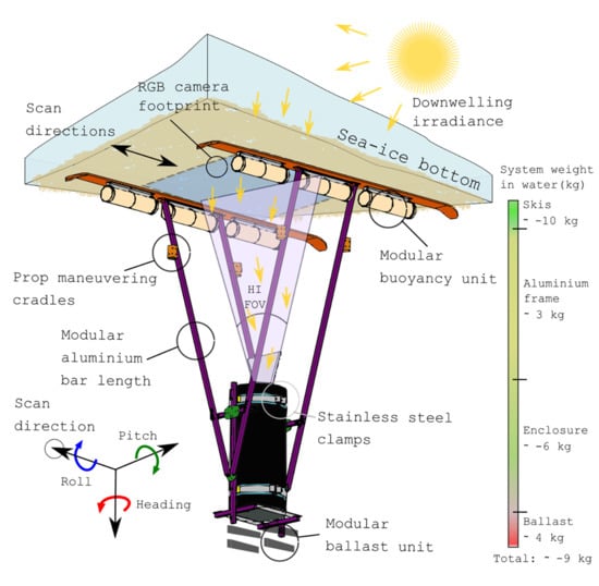
The developed approach here aims instead to scan relatively smooth under-ice surfaces by sliding or “skiing” at a predefined fixed distance from the ice at precisely controllable speeds (Figure 1). This enables the scanning movement to remain considerably stable, reducing some of the requirements aforementioned. The transect is prepared to be a pre-defined straight-line between 10 to 40 meters in length, limited in this prototype by the length of tether (Figure 2). Ideally, the set-up is expected to permit stable scanning speeds matched to the low-light levels experienced and the need of pushbroom HI orthorectification to be suppressed (or minimized). To achieve a steady, slow, and controllable movement, two WG1500 manual worm gear winches (Dutton Lainson, NE, USA) were established at each end-point of the surveyed transects (Figure 2). Stainless steel wires were attached from each winch to the respective end of the aluminum frame legs of the payload rig, which allowed the system to precisely slide back and forth through controlled winch rotations (Figure 2).
Such a sliding concept is only possible on under-ice surfaces which are relatively flat—a common feature of land-fast sea ice in both the Arctic [20,47] and in Antarctica [48]. Fast-ice is not only a relevant target for first tests of the technology, but also provides a relatively simpler optical set-up where algae are mostly residing at the bottom of the ice, at least during spring [14]. Under rougher under-ice surfaces (e.g., pack ice, platelet ice, ice fissures, and cracks caused by pressure ridges or medium to large brinicles) the scanning advancement of the system result could be impeded with such a skies-based concept.
Figure 3 displays the core components of the internal payload that were fitted in the system enclosure. An overview of all sensors, equipment specifications, and their purpose for this first test can be found in Table 1. Detailed information of technical design and software employed to operate the payload can be found Appendix A. The appendix also includes a schematization of power supply and data transmission paths from the surface elements to the enclosure interior and the external payload (Figure A1).
To select an appropriate distance between the imaging sensors and the ice, we considered the trade-off between HI and RGB imaging specifications together with a series of environmental and logistical constraints (see [4] for a trade-offs overview). For example, spatial resolution and image footprint are inversely correlated since increased distances from the ice yields a larger footprint at the cost of pixel size. Increasing the distance from the ice also enlarges the depth of field (DOF), which is an important factor to consider for close-range optical HI and RGB imaging applications. The DOF should be large enough to cover at least the sea-ice skeletal layer where most of the algal biomass is concentrated. Nonetheless, while gaining distance from the ice seems appealing to increase survey area, it increases logistical and technical problems which are relevant to the deployment of a large sliding platform beneath thick ice cover. Such problematics add up to the known effects of the water column on measured light intensity and spectral composition in the visible range [49]. Overall, the increased costs of deploying optical sensors underwater need to be considered together with the additional challenges of geometric and chromatic correction of underwater images associated to the diverse refractive indices across the seawater-glass-air interface [50,51,52]. Such aberrations are not trivial to correct and depend on multiple factors such as the sensors optical parameters and settings, deployment mode (e.g., distance from the ice and field of view (FOV) inclinations), water optical properties and the underwater housing lens design (e.g., flat versus dome), and material (e.g., thickness of the acrylic window).
For this prototype test, we found that an enclosure with a flat-port fitted with sensors separated approximately one meter from the ice would be a good compromise considering our equipment, deployment capabilities, and the spatial variability of the target (sea-ice algae) that we were surveying (Figure 3). The custom-built and low-cost aluminum frame that set the distance from the sensor to the ice was approximately 1.20 ± 0.10 m in length (variable by changing the angle of the legs and steel clamps position). It also allowed the legs to be modified to any desired length if required (Figure 1 and Figure 2). The span between the 1.48-m-long skies ranged from 0.82 to 1.2 meters. It was confirmed that no components of the frame or skis interfered with the sensors FOVs and that FOVs of both sensors largely overlapped for coherent HI and 3D data interpretation.
Since the system travels at a fixed distance from the target, the horizontal and vertical footprint of the sensors can be estimated for the entire transect using standard imaging formulas (e.g., see Appendix B in [24]). Nonetheless, a flat-port causes magnification of images due to the multiple refractions at the air-acrylic-water interfaces, thus reducing the apparent FOV [51]. The amount of magnification is generally ≤1.33 and can be theoretically obtained using Snell’s law. However, such calculations are not straightforward and require a series of sensor optical parameters and sensor specifications, not always easily retrievable. Some include entrance pupil distance relative to the port and imaging object, underwater focus distance and port thickness, among others. To precisely calculate the sensor footprint on the ice, a simpler way is to image objects of known length from which we can retrieve pixel size and derive horizontal and vertical footprint thereafter.
Finally, it is important to consider that miniaturization of remote sensing payloads is always preferable but is inevitably associated with increased cost and/or complexity [28,29]. We must then consider logistical and technical constraints as significant factors that could impede the deployment of a cost-effective solution. It was also preferable to use commercially available and off-the-shelf components when possible, to foster ease of replicability. For example, it was considered mandatory for the system to be surface powered and to be able to stream data to operator and change sensors acquisition parameters based on observed circumstances in real-time. The latter is not straightforward, considering a large amount of data is generated over the multiple high-frequency imaging processes. Costly underwater fiber optic connectors and tethers were avoided by allocating an internal digital processing unit (DPU) within the enclosure, which directly interfaced with the multiple sensors and allowed for on-board data storage (Figure 3). Power and communication with the surface was enabled through an ethernet/power cable permitting for virtual network computing (VNC). Altogether, these design features come at the cost of payload volume, and the entire payload was fitted into a cylindrical enclosure with an internal diameter of 0.23 m and a length of 0.6 m (Figure 3).
The overall height of the system (including the frame legs and skis—Figure 1) was approximately 2 m which required a well-regulated buoyancy to keep the system vertical and pushing against the ice with moderate upward pressure to allow for smooth scanning. This was achieved through modular buoyancy and ballast units that regulated the system’s vertical buoyancy and stability based on local conditions as displayed in Figure 1.
One benefit of the system’s frame size was that it allowed the incorporation of external sensors in the future. For example, for our first tests, we included an upward-looking TriOS Ramses ACC-VIS spectrally resolved irradiance sensor near the ice-water interface to measure light directly exiting the sea-ice matrix (seen in Figure 2 and specified in Table 1).
2.2. Field Site and Transect Preparation
First trials of the system occurred during November–December 2018 under highly productive Antarctic land-fast sea ice off Cape Evans (77.6371733°S, 166.4018691°E) [13,14,48]. As seen in Figure 4c, we did not experience any platelet ice during the period of our surveys, contrary to what was experienced over the same site during other studies [23,48]. The area was characterized by a relatively homogenous sea-ice thickness of approximately 1.8 ± 0.01 m, except for ridged or cracked areas, and this was confirmed by our sampling. The area was also largely snow-free due to wind-induced snowdrift and displacement. An ice hole site was selected from which three transects with variable surface conditions could be surveyed. Transect directions pointed towards northwest (NW), west (W), and southwest (SW). In this study, we provide only a data sample from the western transect as this paper aims to describe the technical performance of the payload and its potential for research applications (see objectives). The analysis of the remaining transects and biophysical investigation of the under-ice habitat at Cape Evans will be presented in a later study.
The 2 m by 1.8 m ice-hole was made through a combination of 6” Jiffy auger holes and hot-water drilling. A polar haven tent was erected on top of the hole to maintain a safe and constant-temperature working environment for the equipment. To create a tow-line for the winch system, a 6” Jiffy auger hole was drilled at the end-side of each targeted transect. From this hole, a rope with a deadweight was immersed and rendered visible from the under-ice. A Seabotix LBV-300 ROV (Teledyne Marine, Seabotix, California, USA) equipped with a grabber arm was deployed from the central hole to grab and retrieve the tow-line from the smaller hole at the end of the transect (Figure 2). Following the installation of the winches, the rope was replaced with the winch wire and this was attached to the under-ice sled.
2.3. Deployment and Data Acquisition
The AK10 only allows for manual focus, and the system does not currently have the capability for remote focusing. The focus distance was required to be set to the predefined scanning distance of the system of approximately 1.2 m. Nonetheless, we need to consider that the focal distance and DOF have the potential to change underwater under a flat port set-up to ultimately affect image sharpness. We, therefore, used an underwater focusing target immerged in the ice hole together with a dummy acrylic glass port to focus the camera under dry conditions while mimicking the underwater optical set-up. The Sony a6300 interface allowed for remote autofocus.
We selected sunny and completely cloud-free days for our deployments to maximize under-ice transmitted light (and thus HI SNR). Before deployment, the enclosure was vacuumed using a standard vacuum pump and PREVCO vacuum kit manifold assembly to an internal pressure of −15 in.-Hg in gauge for leak testing and to reduce internal condensation risks. Although the air in Antarctica is typically very dry, this process is important to avoid any condensation within the enclosure due to the considerable heat produced by sensors and equipment compared to the exterior temperature.
Due to its voluminous shape and weight, the system required two to three people to be manually deployed into the ice hole. The system was then manually pushed below the 1.8 m thick sea ice by two people using rods inserted into the incorporated cradles (see Figure 1 and Figure 4b). The system can then be rotated into the desired transect direction (e.g., western).
Once under-ice, the system was winched three to four meters away from the hole and the tent to avoid interference in the light conditions beneath the ice. We were able to speed up the worm gear winches (designed to be slow for data acquisition) using a winch adapted electric drill as seen in Figure 4d to move the system into the right position for data collection. An initial assessment of the HI signal intensity from directly under-ice was then performed. The optimal traveling speed and HI and RGB imaging settings were then maximized for both SNR and image quality.
The AK10 data storing and imaging settings, including integration time, imaging frequency, spatial, and spectral binning were controlled in real-time using the Lumo Recorder software (Specim Spectral Imaging, Oulu Finland). For HI, the spatial and spectral dimensions were binned to 1024 spatial pixels across track, and a spectral resolution of 3.5 nm (178 bands), respectively. Whilst the spectral dimension could have been further binned to 7.5 nm for increasing the signal; this was avoided as too coarse spectral resolutions are known to hamper the application of some of the HI processing methods for ice algae [27]. The HI frequency was set to 10 Hz and an exposure time of 99 ms (maximum setting available). The ideal sled system speed for these settings was found to be around 0.008 ms-1 corresponding roughly to one rotation of our worm gear winch per second. The read-out frequency of the IMU was also set to 10 Hz aiming for HI and IMU data time-stamp synchronization at the decisecond (ds) level. The survey distance of 1.18 m between the HI sensor and the ice resulted in a HI footprint width on the ice of approximately 0.61 m and a pixel size of 0.00625 m. The Lumo Recorder software was programmed to acquire 100 samples of a dark frame image with the shutter closed at the end of each acquired hyperspectral image. Dark frame images were taken for the subsequent radiometric correction of the imagery through the removal of dark current noise.
The Sony a6300 is operated through the Sony Imaging Edge software “Remote” feature. The software allows live streaming the camera view and permits exposure control, ISO, time-lapse shooting interval, and AF settings to be modified. We found that at the selected winch speed, an imaging interval of 0.1 Hz was sufficient to guarantee abundant forward overlap (>90%). This relatively large sampling interval, together with the slow movement allowed the camera to be set to AF, which resulted in sharp and focused images. The ISO was set to 250; aperture maximized to f/2.8 and shutter speed set to 1/250 sec for most of the circumstances. The altitude of the camera was around 1.2 m, which yielded an estimated footprint width of 0.586 m in water and a resolution of 0.0001 m. All images were captured in the Sony RAW format (.ARW) to allow for any eventual image pre-processing approaches (e.g., see appendix in [24]).
The radiometrically calibrated Ramses ACC-VIS was synchronized to acquire an under-ice irradiance sample at the same time as each Sony a6300 RGB image (0.1 Hz) was taken. In this way, it is possible to link every image to a Ramses ACC-VIS radiometric irradiance sample and locate images spatially across the transect through the retrieved camera positions following SfM digital photogrammetry.
The STS-VIS radiometer was set-up to acquire a measurement of incoming downwelling solar irradiance every minute considering the highly stable conditions during the surveys and the relatively low variability in sun angle.
Following system retrieval, HI, RGB imagery, and IMU navigation data files were downloaded directly from the SATA SSD within the DPU. VNC allows for direct data transfer from the payload to the surface, but the operation is time-consuming for large files such as the HI imagery data files.
2.4. Data Processing
Both hyperspectral image analysis and SfM photogrammetry are active research topics for many land-based applications. The adaptation of established terrestrial procedures to novel under-ice applications requires targeted studies aiming to identify, test, and evaluate their performance in an under-ice context. Here we present only preliminary data outputs of the developed system and assess their quality and potentials from a biophysical perspective. We do this by looking exclusively at the western transect and selecting a successful subsample for hyperspectral image analysis and processing (Figure 5), namely block B. For the RGB imagery and photogrammetry, we retrieve for the first time a high-resolution orthomosaic and DEM of the under-ice using commercially available software. For HI, we adapt some of the known methods in under-ice bio-optical literature to the hyperspectral images and illustrate potential new ones.
2.4.1. RGB Imagery and SfM Digital Photogrammetry
It is well known that image quality and poor camera network geometries can considerably affect SfM model’s reconstruction and the extraction of accurate metric information. Image quality in non-metric cameras is influenced by the camera sensor, lens quality, mechanical stability, and the overall image acquisition process under dynamic conditions. Poor camera network geometry refers to the lack of forward or side overlap in the imagery and/or lack of oblique imagery. Underwater, SfM photogrammetry is further challenged when using flat-ports due to the multiple refraction processes that magnify FOV, affect the focal length and produce a series of geometrical (e.g., radial distortion) and chromatic aberrations in the images directly affecting camera calibration algorithms in SfM, which ultimately affect the reconstructed model.
While image quality, per se, was not considered problematic in our transect dataset, the flat port did cause non-negligible effects on the imagery (e.g., noticeable pincushion distortion). To solve such aberrations and obtain an accurate camera calibration one can formulate the complex mathematical models of the imaging process in water [53,54] or perform a rigorous camera calibration using underwater targets with precisely known geometry [55]. Another option is to rely on camera self-calibration, which refers to the calibration process using only image point correspondences for large and well-composed datasets [56,57]. However, self-calibration is challenging in our dataset as camera network geometry is particularly weak when dealing with elongated strips with only nadir images and no side overlap and/or oblique imagery [57]. Systematic errors produced in such datasets can cause bending and non-linear deformations in the photogrammetric models as confirmed by our tests [57,58]. Here we apply a simple preliminary solution to the camera calibration problem using a constrained self-calibration approach by taking advantage of the flat under-ice surface, the known transect lengths and a series of identifiable reference points that were also measured from above the surface.
Prior to photogrammetric processing, 733 Sony RAW images acquired for the western transect were first imported into Adobe Lightroom where an initial lens correction and manual batch compensation for pincushion distortion was performed. Lightroom considers camera lens profiles into its corrections, and this empirical “trial-and-error” approach is simply to partially reduce bending of the model to a near straight level. Duplicate images were discarded as labeled repetitions during sled idle times, and the remaining images were exported from Lightroom as .JPG files for further SfM processing.
The 3D reconstruction of the under-ice surface was created using Agisoft Metashape (previously Photoscan), is a software package which has been extensively used for 3D modeling and photogrammetry over a wide range of geoscience applications [59,60]. The workflows for under-ice DEM and orthomosaic generation are described here. Photo alignment accuracy was selected as medium (for computational reasons) and provided a first estimate of camera calibration parameters and the reconstructed scene. The produced sparse point cloud model at this stage was noticeably bent and deformed. We proceeded to filter outlier’s and low accuracy points using the gradual selection tools. Due to the smooth nature of the surface (Figure 4c), we assumed that all the surface areas with little algal cover were level with a reference height of 0.0 m, and created a dense and well-distributed network of reference level markers with a Z position (altitude) 0.0 m. We also added the known transect length as a scale bar length reference together with a series of points that were identifiable and could be referenced to above surface positions whose relative position could be measured with a measuring tape. For our entire western transect, we allocated 32 of these reference points, termed ground control points (GCPs) [61,62].
All these level reference GCPs are assigned with a high marker accuracy of 0.002 m in Metashape reference settings options. The model is then processed using the optimization of camera alignment feature where non-linear deformations can be removed by optimizing the estimated point cloud and camera calibration parameters based on these known reference marker coordinates [59]. During this optimization, Metashape adjusts estimated point coordinates and camera parameters minimizing the sum of reprojection error and reference coordinate misalignment error.
The Metashape workflow is then followed by dense cloud reconstruction (medium quality and aggressive depth filtering), 3D mesh from the dense cloud (Arbitrary surface type, medium quality, enabled interpolation, and aggressive depth filtering), texture mapping (orthophoto mapping mode and mosaic blending mode), and finally DEM and Orthophoto production. The scaled orthomosaic and DEM were exported in .TIF format to QGIS and the DEM was processed with a hillshade function for visualization purposes.
2.4.2. Hyperspectral Imaging and Radiometer Data
The retrieved HI images of block A and B consisted of a three-dimensional (x, y, λ) data cube where x and y represent the spatial dimensions, and λ the spectral dimension. The first two steps of the HI processing workflow include radiance conversion of digital numbers (DN) and pushbroom image rectification. The system was designed so that little to no geometric rectification and IMU data integration is required. This was the case for block A and B of the analyzed transect (Figure 5).
Per-pixel radiance conversion was done using Specim Caligeo PRO software (Spectral Imaging, Specim Ltd., Finland) which addresses noise and geometric aberrations inherent to the sensor and performs the conversion of DN into downwelling spectral radiance Ld (λ, mW m2 sr−1 nm−1) using the in-situ acquired dark current frames and the associated calibration files. For the present study, spectral bands <400 nm and >700 nm were considerably noisy and outside the range of interest, therefore spectral subsetting was applied reducing the data to a total of 89 bands.
The block B HI subsamples are then smoothed using a Savitzy-Golay low-pass filter with a polynomial order of three and frame length of nine aiming to reduce noise in the transmitted signals without hindering the retrieval of fine spectral features [63,64].
Following this procedure, we adapted methodologies previously applied to track biomass variability from under-ice spectra such as normalized difference indices (NDIs) and principal component analysis (PCA) (also known as EOF) [5,17,19,27]. Every pixel within the HI subsample was integral-normalized to reduce the amplitude component of spectral variability and to focus on differences in spectral shape, a pre-processing standardization method previously applied in sea-ice bio-optical literature [8,19,48].
PCA for hyperspectral remote sensing is typically employed for dimensionality reduction, to reveal complex relationships among spectral features or for the identification of prevalent spectral characteristics. PCA has been widely used in optical oceanography for extracting information about seawater constituents from spectral data (e.g., [65,66]). In our case, PCA was applied to the spectral dimension of block B data cube to explore and highlight the most variable features and relationships across all pixels in the block B image [27,67].
Spectral indices, such as NDIs, have been linearly correlated to the logarithm of sampled chl-a in multiple sea-ice studies [5,19,48]. Since we have not developed a specific spectra-biomass relationship for our site that applies to the developed HI payload yet, a couple of identified optimal NDIs from the land-fast sea-ice of Davis Station and McMurdo Sound, Antarctica by [48] were selected and utilized as a proxy of biomass. Before index implementation, block B was spatially binned to two by two pixels, reducing the spatial resolution from 0.624 mm to 1.2 mm, but boosting per pixel signal. The following NDI equation was then applied to every pixel in the image:
where λ1 and λ2 are wavelength bands selected across the sensor spectral range and Ld (λ, mW m2 sr−1 nm−1) is the solar downwelling radiance transmitted through the ice. From [48], we selected 441:426 nm and 648:567 nm as two different NDIs in different areas of the spectrum and applied the NDI equation to every pixel in the block B image. In this study, we used radiance to compute the indexes rather than under-ice radiance normalized to surface irradiance (or transflectance [68]). Changes in above surface illumination conditions (e.g., solar geometry and atmospheric effects) within the block A and B image subsample were considered negligible.
In addition to adapting PCA and NDIs to under-ice HI, we also tested for the use of an index called Area under curve Normalized to Maximal Band depth between 650–700 nm (ANMB650–700) of the continuum removed spectrum [69]. ANMB650-700 has been successfully applied for chl-a and chl-b mapping using HI of Norwegian spruce trees [69] and Antarctic moss beds [70], and here we use it as a proxy of chl-a or ice algal biomass.
For this index, we applied the same Savitzky-Golay low-pass filter and the two by two spatial binning factor, but no integral normalization is performed. Instead, the entire image is normalized by the highest spectrum intensity within the block, which corresponds to an algal free cavity in the ice visible in the image (shown later in the results section). This provides a proxy of light transmittance over roughly the last 5 to 15 cm of ice bottom and enhances visibility of the absorption peak of chl-a at 670 nm of each pixel spectrum. The continuum removal transformation on the spectrum is a fundamental pre-processing step to enhance and standardize the specific absorption features of biochemical constituents [71]. It allows for the normalization of the transmittance spectra so that individual absorption features can be compared from a common baseline. Following a localized continuum removal, we can calculate the Area Under Curve in the range between 650 and 700 nm (AUC650–700) where chl-a attains one of its absorption peaks:
where and are values of the continuum-removed transmitted spectra at the j and j+1 bands, and are wavelengths of the j and j+1 bands, and n is the number of the used spectral bands. We can then calculate the ANMB650-700 index as:
where MBD650–700 is a Maximal Band Depth of the continuum-removed reflectance, generally at one of the spectrally stable wavelengths of strongest chl-a absorption around 670–680 nm. Normalization of AUC650–700 by MBD650–700 is a crucial step for strengthening the relationship between ANMB650–700 and the chl-a content for higher chl-a concentrations. The logic behind this spectral index is exploiting well-known changes of the transmittance signature shapes produced within these wavelengths mainly by the changes in algal chl-a content.
In order to validate the robustness of the HI data compared to traditional means of acquiring under-ice spectra, hyperspectral irradiance variability measured with the Ramses ACC-VIS across the entire transect (samples shown as black dots in Figure 5) was computed and compared with spectra of every pixel in block B. The Ramses ACC-VIS data further allow us to gain an estimate of downwelling irradiance intensity exiting the ice-water interface and was used to gain an insight of the light levels experienced under-ice. These can then be used to baseline the signal quality of the data achieved using our HI system under those specific conditions. The TriOS Ramses ACC-VIS was radiometrically calibrated using the factory provided calibration files (traceable within international standards) during the data acquisition process.
3. Results
3.1. Deployment and Operation Performance
The system was successfully deployed and retrieved for the three targeted transects (NW, W, and SW). For the western transect analyzed here, a total of 736 RGB images and Ramses ACC-VIS irradiance samples were acquired, in both forward and backward directions (Figure 5). The overall scanning operation lasted approximately 2.5 hours, not including system set-up. Considering the air (–5 to 5 ℃) and water (–1.8 ℃) temperatures experienced, the electronics in the housing functioned well under the challenging environmental conditions and were kept above freezing point by heat produced from the multiple electronics. HI-sensor temperature sensors indicated that temperature was maintained at around 17 ℃ over the entire western transect.
As shown in Figure 6, the system was able to produce natively well-composed pushbroom hyperspectral images without the need for any rectification methods and/or additional attitude and navigation data (e.g., see block A in Figure 6c).
However, occasional lagging instances in the sled-motion during scanning of some sections of the transect hampered smooth pushbroom HI data acquisition. Sometimes these lags were long enough (0.5–3 seconds instances) that data collection had to be interrupted and the sled system to be forwarded until the movement was smooth again. In other cases, they were acceptable and could eventually be corrected through the integration of the IMU data algorithms and image correction filters (e.g., Figure 6 lagging instance). Transect blocks requiring rigorous geometric rectification and post-processing are out of the scope of this study and will be investigated in the future through the development of targeted geometric HI correction algorithms.
Transects also did not always followed a straight line, but instead, the trajectory displayed a slight bend as can be seen from Figure 5. This means that the system showed changes in heading according to its attitude reference system (heading, roll, and pitch) shown in Figure 1 and Figure 3. Transect bending is only noticeable when considering long distances rather than over the shorter accomplished HI scans. However, this track deviation did have an impact on the imaged transect as forward, and backward travels did not perfectly overlap in some instances producing unnatural invasive marks such as the visible ski tracks in Figure 5.
3.2. RGB Imagery and Photogrammetry
For the western transect, 615 camera positions were aligned successfully, and optimization produced an overall flat 3D model of the under-ice surface (Figure 5 and Figure 6a). Dense reconstruction of the model resulted in a rich and well-composed dense point cloud (100,199,561 points). The first estimation of the total area covered was 13 m2 for the western transect. The final resolution of the displayed orthomosaic was 0.0994 mm/pixel and for the DEM 0.821 mm/pixel with a point density of 1.48 points mm−2. The total RMSE of the Euclidean distance between the generated reference level markers and the corresponding estimated points in the reconstructed 3D model was 0.0762 m (0.0623 m X error, 0.0322 m Y error, and 0.0297 m Z error). While this error does not reflect a rigorous accuracy assessment of the absolute geometric accuracy of the model, our interest in these first trials was in the ability to retrieve complex topographic features. The relative (within model) accuracy and point density are sufficiently high for this purpose.
The RGB orthomosaic illustrates the high level of algal biomass under the land-fast sea ice of Cape Evans. This encompasses both gentle changes in illumination and also different shades of brown and green coloration over the full 20.1 m transect (Figure 5). Zooming into block A, Figure 6a displays complex networks of ice algal aggregations and patches together with the presence of large bright cavities embodying large secondary brine channels [72]. The DEM hillshade in Figure 6b shows that while at first sight, the under-ice at Cape Evans seems like a featureless surface, it has high levels of relief complexity attributed mainly to an extensive network of secondary pore spaces [72]. Looking at Figure 5, they appear to occur in specific areas of the western transect. These pore cavities range widely in size and depth and are believed to be a result of a series of sea ice thermodynamic processes of brine flushing and merging of channels during the advancement of the summer season (e.g., [72,73]). An ice core footprint of 0.14 m in diameter is provided as a reference scale for these large brine pores in Figure 6a,c. However, the total depth of the cavities is difficult to capture with digital photogrammetry, and we could only image and reconstruct up to a certain depth depending on their width. Smaller subtle relief and undulations of the under-ice surface are also observable from the DEM hillshade (Figure 6b). Since these are not recognizable as white spots from the imagery itself, they are perhaps not strictly related to brine release processes but rather ice undulations of yet unknown origin. The DEM hillshade also captures micro-rugosity in the 3D model attributed to protrusion of dense algal clumps mostly formed by the diatom species Berkeleya adeliensis (F. Kennedy pers. communication). The hillshade map also displays a specific orientation pattern assumed to be driven by the underlying water currents. Berkeleya adeliensis was found to be the predominant species together with the interstitial diatom Nitzschia stellata from microscopic observations.
Current-driven orientation of algae strands and the biophysical complexity of the under-ice habitat were also observed in the high-resolution Sony a6300 RGB images shown in Figure 7. These images not only display the native quality of the RGB imagery but also show additional important biophysical properties of the under-ice habitat such as the sea-ice skeletal layer and its crystal orientation (Figure 7a) [72,74]. Figure 7a was taken nearby the ice hole, and the difference between what appears to be the hanging Berkeleya adeliensis and interstitial diatom species is clearly visible. Later into the transect in Figure 7b, a certain degree of algal orientation can also be observed together with some of the large secondary brine channels. Zooming in on Figure 7b, we also observed high concentrations of oxygen bubbles produced by the photosynthesizing algae. Also, several types of under-ice fauna were visible along the high-resolution imagery dataset such as ctenophores (Figure 7a) and amphipods (Figure 7b).
3.3. Hyperspectral Imaging and Radiometric Data
A visual representation of the block A hyperspectral data cube within the western transect is shown in Figure 6c. The quality of the image composition shows minimal geometric noise and a robust geometrical resemblance with the RGB orthomosaic for the entire block A subsample. The cube also shows an example of one of the lagging instances in the sliding sled system as previously noted.
The right-hand plots in Figure 6 display the quality of the measured spectral signatures in terms of overall intensity for the under-ice downwelling radiance Ld (λ, mW m2 sr−1 nm−1) unprocessed (Figure 6d) and smoothed (Figure 6e). It is clear that high variability of light intensity and spectral shape can be found across a series of features within the <1 m2 area of block B. Such variability can change up to one order of magnitude and is mostly ruled by the presence of the secondary brine channels together with the drastic differences in algal concentrations and aggregations, but also due to the different algal species/morphotypes (e.g., hanging versus interstitial) among other factors. Despite the highly contrasting under-ice light regime induced by the large brine features, the camera dynamic range allowed to optimize settings to the lower light areas (e.g., algal patches) without saturating the pixels over the secondary brine pores.
Absorption by algal associated chl-a is easily observable over almost all pixels in the image as a reduction in intensity over the 440 ± 20 nm and 680 ± 10 nm bands. Higher ice algal biomass reduces transmitted radiance in the blue part of the spectrum and produces a compressed curve in the green part of the spectrum [75]. Absorption features by ice algae tend to drastically decrease nearby and within the secondary brine channels (e.g., red spectrum in Figure 6d–e) except in circumstances where we find dense algal webs hanging in the middle of these cavities (e.g., celeste spectrum in Figure 6d) or highly concentrated algal clumps scattered around these cavities. From the entire block A image, we also selected some of the lowest light pixels we could find, and their spectrum can be seen in Figure 6f. The SNR noticeably decreases for such targets, and the blue region (400 to 500 nm) seems to be noise dominated. Nonetheless, the spectrum still displays strong chl-a signatures in the 680 ± 10 nm band curve and an overall meaningful signal.
The mean irradiance spectrum ± standard deviation (sd) measured with the Ramses ACC-VIS for the length of the whole 20.1 meters transect is shown in Figure 8a. The total irradiance energy integrated over the PAR range (400–700 nm), Ed,PAR (λ, W m2) averaged 0.35 (λ, W m2), with a 0.20 sd, and a total range of 0.07–1.5 (λ, W m2). Figure 8a also helps to characterize the spectrum variability across the entire transect. Interestingly, a similar degree of variability (although in terms of radiance) is experienced within the <1 m2 block B subsample as seen in Figure 8b showing the mean spectrum ± sd of all pixels of block B. Figure 8c displays the integral-normalized mean spectrum of all the pixels of the block B hyperspectral data cube overlaid by the integral-normalized mean spectrum of the entire western transect using the Ramses-ACC-VIS. Figure 8d displays all pixels of the block B image normalized by the highest light intensity pixel in the images which is attributed to the light exiting one of the secondary large brine channels or cavities (seen Figure 6). This plot indicates properties of the transmitted light over the bottom layer of the ice where >98% of the biomass thrives. The normalized spectra were used to compute the ANMB650–-700 index. The normalization greatly accentuates the absorption features of chl-a in the blue area centered at 450 nm and the red peak centered around 670 nm.
PCA results are shown in Figure 9. The loadings of the first nine principal components explaining >99.54 % of spectral variability within the image are shown for completeness. Figure 8 also displays the loading scores applied to each pixel of block B for the first three principal components (PC1, PC2, and PC3) together with an RGB composite of block B. PCA results show well resolved and coherent principal components similar to what was reported previously in the literature employing PCA (or EOF) using under-ice radiance and irradiance sensors in-situ [5,19], or for HI in artificial sea-ice simulation tanks [27]. The PC1 loadings account mainly for variability in light intensity attributed to a mixture of factors and embody the general trend of the under-ice light spectrum. PC2 seems to be more influenced by the two contrasting dip areas around 440 ± 20 nm and 680 ± 10 nm suggesting a possible correlation with algal chl-a pigments. Nonetheless, PCA at this stage serves as an exploratory tool and it remains difficult to assess the nature of PC3 and the remaining PCs without further analyses of pigment composition e.g., through high-performance liquid chromatography (HPLC) (e.g., [43,48]). The PCA score images also evidence some subtle line artifact features across the scanning direction of the hyperspectral image (Figure 9). These are attributed to small vibrations or micro-lagging instances whose visibility is enhanced following integral-normalization and PCA processing.
The results of the NDI (648:567 nm) and ANMB650–700 indices applied as relative proxies of biomass variability to block B are presented in Figure 10a,b, respectively. Interestingly, Figure 10 suggests that both indices provide a similar result in terms of biomass distribution patterns and capture spatial scales previously unprecedented. However, NDIs seems to produce nosier images compared to ANMB650–700. It might be argued that the ANMB650–700 is based on the curve shape information of the light transmitted through the algal layer and such normalization was not applied to compute NDIs. However, both methods were tested and showed that using quantitative changes of transmitted radiance intensity produced less noisy images in case of NDIs.
NDIs applied to block B over the blue/violet area (441:426 nm) were also tested and provided similar results although with slightly noisier imagery (not shown). A final interesting observation is the anisotropic noise pattern observed in both NDIs (648:567 nm) (Figure 10a) and PCA across the scanning direction of the image (Figure 9). This is observable as noisier zones at the top and bottom of the image.
4. Discussion
4.1. Under-Ice Hyperspectral Imaging Data Quality and Processing
The present study outlines a novel platform incorporating two emerging underwater optical methods for capturing fine-scale biophysical properties of the under-ice habitat non-invasively. Passive HI and digital photogrammetry were tested for the first time to observe the ice-water interface and were deployed using a relatively simple under-ice sled. The sliding concept took advantage of the fixed and smooth surface of land-fast sea ice to minimize costly set-ups and yielded geometrically coherent hyperspectral imagery without the need of georectification. To the authors knowledge, only three underwater HI payload designs have been documented before. The Ecotone UHI (Ecotone, Trondheim, Norway) is a commercial solution designed for deep or shallow ROV-based seafloor observations and utilizes active light sources [36,76]. The Ecotone UHI has also been equipped onto unmanned seafloor vehicles (USV) for shallow seafloor mapping [33]. The other two are documented in [32,34] and comprise of stationary time-lapse observations and a diver-operated set-up.
In terms of data processing, the aim was to provide a preliminary outlook of the system’s data outputs and its potentials. The preliminary results presented here indicates that it is possible to apply simple, yet effective, algorithms to retrieve chl-a per surface area on a sub-mm per pixel basis over tenths-of-meters-long transects. Figure 8 shows that the under-ice spectral signatures of traditional and novel sensors are comparable. They are also comparable with studies over similar Antarctic land-fast sea-ice areas (e.g., [48]). Established under-ice bio-optical methods for retrieving sea-ice biomass proxies in-situ (e.g., NDIs or PCA models) were also successfully adapted to the acquired hyperspectral imagery (Figure 9 and Figure 10). NDIs values outputted are observed to match the range of values over the same or similar sea-ice areas [48] and PCA loadings shown strong similarities in shape if compared with results from other studies both in real sea ice and in artificial ice tanks [7,27]; the difference being that in this study they were retrieved on a sub-mm per-pixel basis.
PCA results retrieved chl-a signatures over its PC2 component and reaffirm the utility of PCA for explorative analyses. For example, the pronounced “shoulder” deviation towards 470 nm in PC2 loadings is likely associated with a higher concentration of accessory algal pigments such as fucoxanthin [77,78]. PCA analyses also suggest the possibility to retrieve PC/EOF based regression models to develop chl-a-spectra relationships, algorithms that have been proven successful for a wide range of sea-ice conditions [5,19,27].
The use of the NDIs positioned at wavelengths 648:567 and 441:426 nm was also tested with meaningful per-pixel biomass proxy representations although images were characterized by consistent pixel noise, particularly for the blue region of the spectrum (Figure 10). This is probably attributed to the lower SNR inherent to mm-scale hyperspectral resolution image pixels compared to wide-footprint radiometric sensors. SNR changes due to variations in intensity and shape of the retrieved spectra, which varies as the target constituent concentrations change and as the noise changes depending on sensor settings and specifications. The high ice algal biomass typically found at Cape Evans (see [1] for biomass ranges), favors algal associated spectral shapes, but heavily reduced light availability and consequently per pixel SNR on the overall spectrum, particularly in the blue region where chl-a attains one of its major absorption ranges (e.g., for the NDI 441:426, see Figure 8b,d). In fact, from Figure 10a, we can observe how noise is drastically reduced over the high light intensity brine channel areas. Studies [48] and [22] also highlighted how in general NDIs were producing poor relationships at the Cape Evans site. However, this might be because of different reasons such as the presence of platelet ice (which we did not experience during our study), the consequent poor spatial variability in biomass at the measured scale, or perhaps the difficulty in ice-coring and sampling chl-a from sloughing platelet ice [22].
The ANMB650-700 index explored here is directly linked to the absorption properties of chl-a in the red region of the spectrum. It takes the advantage of hyperspectral data to finely integrate over the narrow absorption peak of chl-a in the 650 to 700 nm range. While it is not guaranteed that a meaningful quantitative relationship with sampled chl-a will be retrieved, the index performed better than NDIs for our case by providing less noisy and coherent images (Figure 10b,c). Increases in chl-a concentration (with absorption maximum around 665 to 680 nm) causes chl-a absorption feature to deepen at the 680 ± 10 nm dip. While the spectrum of the transmitted radiance in this range can show signs of saturation, the adjacent wavebands at longer wavelengths remain sensible to changes as the peak broadens and thus extending the area under curve (Figure 10c) [69]. The index was also designed to reduce the impact of other confounding factors of the imaged target within its complex 3D environment [69], and this might also supported the index performance in our case. A continuum-removed integrative index could also have worked better than a band ratio (e.g., NDIs) under this high biomass case (and therefore less light and SNR) as it integrates a larger area (AUC) hence providing a stronger signal per-pixel (Figure 10c). In fact, the performance of ANMB and similar indices is expected to deteriorate under low chlorophylls (chl-a and chl-b) amounts [69,79].
Future work in this area will explore the performance and comparison of these indices for the Cape Evans site, and to work on the retrieval of quantitative correlations tailored to our encountered sea-ice conditions that are suitable to be applied to HI data. It was also noticed how different pre-processing, normalization, and standardization techniques (not all shown here) affected the visualization of indexes applied to the images and the performance of exploration methods such as PCA. Such observations prompt for the investigation of optimal workflows to process and analyze under-ice HI data.
4.2. System Performance and Future Developments
While most of the transect could be scanned as planned, some issues were experienced during the scanning process such as invasive ski marks and occasional lagging which hampered pushbroom image composition (Figure 6 and Figure 8). Nonetheless, the low gear winch system was capable of delivering extremely slow speeds in a stable manner as observed in the imagery. The observed angular deviations are comparable to data for professional gimbal stabilization systems for UAV applications [80]. They had negligible effects on the HI image composition and RGB imagery in our case due to the close-range set-up and the extremely slow speeds. The only trade-off of the system is that the winches had to be manually rotated which is a time-consuming and personnel demanding process. For future deployments, we plan to automate and motorize the winch system. The changes in transect heading are likely attributed to a combination of small-scale ice irregularities, inhomogeneous surface drag and/or the effect of intermittent currents observed from our underwater footage. There is also the possibility of a loosened ski frame support which went unnoticed. The cause of the lagging could be attributed to these roll changes but could not be precisely identified either. Investigation of the RGB imagery did not point to a particular ice condition that could have induced the lagging. A too strong buoyancy force against the ice (−9 kg in water, Figure 1) might have increased surface drag to a counterproductive level.
These aspects can firstly be improved by developing an improved sliding system and refining its technical design. However, greater advantage is envisaged in exploring manual or automatic pushbroom HI rectification techniques through the incorporation of overlapping RGB orthomosaics, also known as co-registration [81,82,83]. This approach co-registers the hyperspectral imagery based on a reference RGB orthomosaic through image matching procedures (e.g., feature matching and transformation based on matching points [28]). The only requirements for co-registration are spatially similar and overlapping HI and RGB imagery and good accuracy for the RGB orthomosaic reference. Advances in camera calibration and triangulation procedures permit the generation of RGB orthomosaics with high geometric fidelity using a limited amount of GCPs and/or consumer-grade navigation data [60,61,84]. Although a more accurate assessment is still required, the western transect RGB orthomosaic resulted in a highly resolved and metrically scaled photogrammetric model which could be used for co-registration for example (Figure 5 and Figure 6a,b). This was possible as our camera calibration and model reconstruction heavily benefitted from a constant sea-ice thickness and imaging altitude which allowed to impose an artificial network of GCPs of precisely known positions in the 3D space. The same approach would not be possible under highly heterogeneous topographies or would not be as effective for highly dynamic imaging conditions. Under these sub-optimal circumstances, the options could be to retrieve an accurate camera model using underwater calibration targets [39,55], to estimate it through its mathematical formulation and/or to implement the use of dome ports [51]. Another option remains the addition of physical GCPs. Compared to the seafloor, the sea-ice can be used as an opportunistic reference surface where ground control points visible below and above the ice can be allocated (e.g., Nicolaus and Katlein, 2013). GCP positioning can then be accomplished using conventional GNSS devices and manual measuring or by referencing them in a local reference system. This is advantageous as positioning underwater typically requires the acquisition of acoustic data, which may depend on information from the under-ice vehicle/platform to a research vessel through a network of deployed transponders [8,85,86,87]. This process requires considerably more effort and resources and would arguably suit the precision required by line scanning orthorectification methods.
By taking advantage of the referenceable sea-ice surface and co-registration methods we could then theoretically develop algorithms analogous to aerial HI algorithms based on the scaled RGB orthomosaics, the partially rectified HI scans and the acquired consumer-grade IMU data [37,81,82]. These future developments will aim to support the geometric correction of distortions caused by the dynamics of the HI frame, such as the lagging instances (Figure 6c). In addition, robust geometric correction will pave the way for a more independent system that can operate under rougher under-ice topographies and at increased distances from the ice. The system needs to strive towards increased distance from the ice, and ease of operability under diverse under-ice conditions. As the technology develops, there is also potential to drastically reduce the weight and volume of the payload. Eventually, this may allow the development of HI payloads for ROVs or unmanned underwater vehicles (AUVs) to drastically increase the spatial extent of the surveys, although there are physical and technical challenges associated which are briefly discussed in the last sub-section.
4.3. Potential Applications of Under-Ice Hyperspectral and RGB Imaging Payloads
Compared to standard imagery or multispectral imagery, HI provides narrow spectral resolutions, high bit depths, and actual radiometric and referenceable units. Higher spectral fidelity sensors with reasonable spectral resolution would not only be beneficial to produce quantitative estimates of fine scale sea-ice biophysical properties, but also to develop tailored relationships for each study area and move towards more universal approaches and algorithms [4]. The complex under-ice perspective will undoubtedly pose new challenges and constraints. However, several additional indices or machine learning approaches coupled with radiative transfer modelling efforts could be tested and adapted to produce more robust and universal relationships to retrieve diverse biophysical properties. Some examples can be found in forestry and agriculture [29,79,88], ocean color [89,90], chemometrics [67], and other environments [34,91].
Low-cost imagery sensors—such as RGB, near-infrared (NIR) or multispectral—have also served well in multiple close-range remote sensing applications to retrieve qualitative and quantitative information from biological targets [92,93,94]. For the under-ice environment, RGB imagery has been used to qualitatively assess the spatial distribution of algae [9,95,96]. Therefore, RGB or multispectral imagery should be considered from a cost-benefit analysis perspective based on desired research aims and available resources.
In theory, hyperspectral resolution data has the potential to resolve beyond pure biomass estimates towards more sophisticated biological traits such as ice algal photophysiology [91,97,98], species composition [97,99,100], pigment detection [101,102,103], and feature classification and mapping [35,76,104]. An interesting field is also being explored in the retrieval of primary production estimates from spectral data in combination with in-vitro photosynthetic parameters for ice algae [7,105] or with PAM fluorometry for microphytobenthic communities [106].
Compared to point sampling radiometers, the main advantage of imaging payloads is the possibility to capture the information at ultra-high spatial resolutions (in this case sub-mm scales) in a non-invasive manner (e.g., [34]). Under sea ice, this will allow future studies to investigate multi-scale ice-algal dynamics and how they covary with environmental drivers over space and time [4,11,47,107]. With little additional effort, the RGB imagery and close-range digital photogrammetry provided an accessible tool to producing ultra-high resolution orthomosaic and 3D models of the under-ice surface.
Surface topography is a well-known factor driving spatial distributions in many marine ecosystems (e.g., [108]). Under-ice, the potential of high-resolution HI and 3D data fusion could contribute to new opportunities to monitor some of the sea-ice biophysical interactions which were previously difficult to capture. The effects of under-ice topography on sea-ice algal biomass distributions has long been queried and investigated [10,109,110]. Recent studies have further observed and inquired about the role of under-ice topography and underlying currents on algal biomass distribution at multiple spatial scales [11,96,111]. Hydrodynamic shadows can foster the accumulation of diatoms, algal aggregates, and may also provide shelter for under-ice fauna [9,112,113]. The RGB imagery not only can provide under-ice roughness but it could also serve to gain further insight into grazing dynamics by sympagic fauna (Figure 7).
The effects of sea-ice structure and physical properties also go beyond effects on biomass distribution and are known to influence algal photophysiology, species composition, and production [1,3,9,114]. Although intrinsically different from some of the Arctic examples cited above, the dataset presented here clearly illustrates a complex biophysical scene for Antarctic land-fast sea ice even within a square meter area (Figure 8 and Figure 9). For example, we found large secondary brine channels to characterize specific areas of the scanned transect (see Figure 5). These cavities augmented transmitted light conditions that showed localized maxima of up to one order of magnitude (Figure 6). The question arises whether these under-ice features have an impact on algal distribution, species composition, and/or photophysiology, or if they play any role in hydrodynamic regimes and under-ice grazing dynamics. The presented methodology may contribute to a better understanding of some of these complex biophysical interactions.
4.4. Caveats and Future Challenges
Our sliding system has been designed for deployments over relatively smooth under-ice bottoms. Nonetheless, the principles of operation of HI and digital photogrammetry remain applicable to any ice type, provided that under-ice light levels are sufficient. In cases where the sliding concept is not applicable (e.g., rough pack ice), platforms will need to be equipped with sensors to accurately trace HI sensor attitude and dynamics.
In this study, the HI payload was operated under thick (1.8 m) and almost snow free fast ice (Figure 5). To account for low under-ice irradiance levels (0.35 ± 0.20 W m−2) the system was operated at extremely slow scanning speeds (0.008 ms−1). These irradiance values are comparable to under-ice light levels and variability for Arctic fast-ice during spring [68], and help to provide a baseline for the range of under-ice irradiances intensities for which our payload could acquire meaningful HI signals. However, many other sea-ice conditions remain to be explored (e.g., with deep snow packs) and which may pose significant technical challenges. Low light levels will push sensors to their sensitivity limits, necessarily affect SNR and hinder the integration of pushbroom HI payloads onto more efficient and dynamic underwater platforms, such as ROVs and AUVs. A series of studies have already employed pushbroom HI sensors for seafloor mapping using ROVs [35,36,76], diver operated systems [32], or unmanned surface systems [33]. A first study has also discussed HI feasibility onto AUVs [115]. However, these applications positively benefitted from artificial light sources that illuminate the imaged scan line, or were performed in shallow, clear tropical waters. For mapping under-ice environments, there is a trade-off between sensor integrations times, imaging frequencies, and platform dynamicity under low light conditions that will need further investigation [4].
The inclusion of underwater IMUs, relative positioning systems, and implementation of targeted under-ice pushbroom HI orthorectification methods will open up new avenues for this type of research. While active lights sources could be eventually considered for under-ice mapping, the resulting mixture between reflected and transmitted light through a complex and translucent medium would render data processing and interpretation extremely challenging. In fact, our system features a set of artificial light sources as shown in Figure 4b and schematized in Figure A1. Using a custom-built control (Figure A1), the LEDs were tested and observed to provide a slight increase in the measured signal. However, it was preferred for the scans here presented to avoid their use to avoid complicated data interpretations. The effect of strong LEDs on relatively low-light adapted algal communities could also question the invasiveness of the methodology.
Additional challenges arise due to the complex nature of sea-ice optical properties and the resulting anisotropic under-ice light field [116,117]. The anisotropic light field is shaped by the lamellar sea-ice features funneling light in the downwards direction creating a forward peaked light field. Lamellar structures associated with columnar ice were clearly observed in our site (e.g., Figure 7). Analogous above surface HI applications (e.g., equipped onto UASs) have acknowledged the impact of an anisotropic leaving reflectance on the retrieval of biochemical parameters using spectral data [118,119,120]. In this study, we experienced noise artefacts over block B sample processed images as an increase in noise patterns at the upper and bottom edges of the image. This is most likely inherent to camera optical design and sensitivity heterogeneity across the spatial dimension, but it could also be in part attributed to light-field anisotropy. A forward peaked light field could mean a stronger signal at the center of the line scan and a decreasing signal towards the edges of our ~30 FOV. However, other possible causes should be taken into consideration (e.g., data processing artifacts) or the dense oxygen bubble layer causing multiple refraction effects (Figure 7). Eventually, the impact of an anisotropic under-ice light field, or other particular environmental conditions (e.g., oxygen bubbles), on HI data will need to be further assessed, and corrections developed towards improved estimates and interpretations.
We did not apply any corrections for the water column effects to either the RGB imagery or to the HI data processing workflow. This is acceptable as the water column in between the ice and the enclosure was <1.1 m and our site was characterized by exceptionally clear waters (see Figure 4c). Antarctic surface waters are generally considered to have low particle loads with low backscattering (e.g., [121]). Nonetheless, as we increase sensor distance from the target, or in case of consistent under-ice phytoplankton abundance (e.g., [122]), the impact of the water column should be addressed with standard color correction approaches for RGB imagery [44,123,124] and for the water column correction of hyperspectral radiometric data if possible [44,125].
Our sea-ice site also benefitted from optically “favorable” conditions where biomass was high and resided mostly in the bottom 3 cm of the ice. Due to the scattering properties of sea ice, the bottom 3 cm algal layer can be considered as an evenly illuminated “thin” sheet that was scanned with our payload. While ice algal biomass is known to be generally concentrated at the ice bottom, where organisms enjoy more favorable living conditions [1,16], there are many circumstances of vertically variable distributions [16]. Future applications of HI for sea ice with a certain degree of vertical biomass variability (e.g., in Antarctic pack ice) will need to consider these effects. Due to the scattering nature of sea ice, biomass in the sea-ice interior will probably have a negative impact on discernible spatial resolutions and image interpretation. Larger protruding algal filaments that are only loosely attached to the subsurface of the ice could also be a problem under dynamic currents for both HI and RGB imagery. In our case, filaments did not represent a significant problem as they were relatively short and under-ice currents during scanning seemed monodirectional, thus providing a relatively still scene (Figure 7). Finally, the feasibility and performance of HI to capture biomass variability under the extremely different biomass ranges found in the sea ice need to be assessed. A compilation of biomass ranges found in sea ice can be found in Arrigo (2017). A previous experimental study has shown HI to be able to discern biomass ranges as low as 0.036–2.72 mg m-2 [27], but much more work is required to investigate the impact of different concentrations on per-pixel SNR and regression algorithms performance.
5. Conclusions and Outlook
Sea-ice biophysical properties can exhibit high spatio-temporal variability at very fine scales (e.g., <1 m2) which are difficult to capture and quantify using traditional methodologies. In response to some of these limitations, this study has presented a proof-of-concept for using hyperspectral imaging and digital photogrammetry for under-ice habitat mapping using a modular, low-speed sliding platform. The particular “inverted” under-ice perspective poses new challenges and limitations to HI which were thoroughly discussed in this study. We demonstrate that the new system was able to map a ~20 m-long transect with geometrically consistent pushbroom hyperspectral imagery, together with overlapping digital elevation models of the under-ice surface, at sub-mm spatial resolution.
Despite the low light irradiance levels experienced ( = 0.35 ± 0.20 (λ, W m−2)), our HI payload attained suitable per-pixel under-ice signals for employing established bio-optical approaches without the need of active light sources. Minor issues with the sliding system where experienced (e.g., occasional lagging and ski marks), but these seem to be addressable with feasible system modifications and/or data processing techniques.
Future work will aim to address system performance and technological capabilities to increase the spatial extent of the surveys, data acquisition under rougher ice types and investigate pushbroom image rectification approaches based on RGB imagery. RGB imagery and digital photogrammetry were shown to provide ultra-high-resolution DEMs and orthomosaics of the under-ice habitat. RGB imagery presents diverse opportunities to qualitatively and quantitatively map and investigate under-ice objects of interest together with highly detailed under-ice roughness.
For under-ice HI, several aspects remain to be investigated prior to method standardization. We think light limitation, the complex under-ice light field, and vertically variable biomass distributions should be further investigated and their impacts on HI methods assessed. For digital photogrammetry, efficient camera calibration approaches should be tested in an under-ice context to assess and improve DEMs accuracy.
Finally, we need to move from relative indices proxies to actual quantitative per-pixel biomass estimates. In this study we only underlined the potential of applying spectral indexes and dimensionality reduction methods to retrieve biomass proxies. We then validated them by comparison with values documented in other studies. The next step is to develop a targeted biomass-spectra calibration suitable and tailored for our sensor payload and study area. This will be eventually applied to the full set of images transect imagery so that we can gain a better understanding of the under-ice habitat characteristics at Cape Evans, Antarctica. We expect that HI systems will contribute to fill a niche gap in the mechanistic understanding of some of the complex under-ice biophysical interactions.
Author Contributions
Conceptualization, E.C., K.M.M., A.L. and V.L.; methodology, E.C. and V.L.; software, E.C.; validation, E.C.; formal analysis, E.C.; investigation, E.C.; resources, V.L. and K.M.M.; data curation, E.C.; writing—original draft preparation, E.C.; writing—review and editing, E.C., K.M.M., A.L. and V.L.; visualization, E.C.; supervision, K.M.M., A.L. and V.L.; project administration, V.L.; funding acquisition, V.L.
Funding
This research was supported under Australian Research Council’s Special Research Initiative for Antarctic Gateway Partnership (Project ID SR140300001), and the New Zealand Antarctic Research Institute (NZARI) under project number K043-1819-A. Emiliano Cimoli is supported by the Antarctic Gateway Partnership and the University of Tasmania’s Ph.D. program.
Acknowledgments
We are grateful for the support of Antarctica New Zealand staff and the K043 team for field-based operation and logistics. We gratefully acknowledge the support of Richard Ballard for circuitry production, and technical support during stages of this project. We are also thankful to several members of the TerraLuma team for valuable advice and support.
Conflicts of Interest
The authors declare no conflict of interest.
Appendix A Technical Design and Specifications
The core equipment of the developed system consisted of an AISA Kestrel 10 pushbroom HI camera (AK10) (Specim Spectral Imaging Ltd., Oulu, Finland), a DPU (Specim Spectral Imaging Ltd., Oulu, Finland) and a Sony a6300 mirrorless digital camera together with a Samyang 35 mm prime lens. Accessories include a Low-Light HD USB camera (Blue Robotics Inc., California, USA) a VN-100 Inertial Measurement Unit (IMU) (VectorNav Technologies, LLC, Dallas, USA) and a Garmin 18x LVC GPS (Garmin, USA). In our independent external payload, we included a TriOS Ramses ACC hyperspectral cosine corrected spectroradiometer (TriOS Mess- und Datentechnik GmbH, Rastede, Germany) and a set of four daisy-chained Subsea Lumen Lights (Blue Robotics Inc., California, USA).
Figure A1 illustrates the power supply and data transmission paths from the surface elements to the enclosure interior and the external payloads. The internal payload is fitted inside an off-the-shelf black anodized cylindrical aluminum enclosure manufactured by PREVCO (PREVCO Subsea, Fountain Hills, USA) that seals via two nitrile O-rings for each end plate and is rated to a depth of 100 m (Figure 3). The end-cap is fitted with a single underwater connector and a pressure release/vacuum hole. The connector used for external communication and power supply with the surface was a 13 contacts circular SubConn power/Ethernet.
Figure A1.
Schematics of the electronic power and communication streams for the internal and the additional external under-ice payloads.
Figure A1.
Schematics of the electronic power and communication streams for the internal and the additional external under-ice payloads.

All components of the payload were mounted around a custom-made vertical aluminum tray (20.32 by 60.96 cm) that hangs from the enclosure end cap for full swift removal and insertion of the payload (Figure 3 and Figure 4a). The umbilical used is a 13 contacts SubConn power/ethernet (Type: D-P-P4TP24#/4C18#, 50 m long) and is received on the surface by another circular 13 contacts connector. Data and power streams were then divided within the enclosure and above the surface from the connectors by unregulated breakout PCBs (Figure 4). The ethernet stream within the enclosure connects directly to the DPU, allowing for VNC from the above surface PC. In our set-up, we used the freely available TightVNC software (https://www.tightvnc.com/) for this purpose. Most sensors were interfaced and powered through the DPU using their respective data/power cables, as shown in Figure 4 and operated through their own software. Only the Sony a6300 was powered using a different route. The power stream within the enclosure went through a power regulator PCB that fed the DPU directly and the Sony a6300 camera via Tether Tools Case Relay (Tether Tools, Phoenix, USA), and a Relay camera coupler for the Sony a6300.
An alternative low-cost solution was designed to synchronize and time stamp pushbroom frames with attitude (roll, pitch, and heading) data from the IMU. The IMU PCB in Figure 4 collected NMEA strings from the GPS and sent them through USB serial connection to the DPU for local time synchronization. The VN-100 IMU uses a 1 PPS sync input from the GPS as a trigger and reference to start its internal timer and to synchronize it to the GPS clock. This means that for each packet of data that the IMU outputs, it stamps the packet with an accurate GPS timestamp. Within the DPU the data is recorded using a Python script (run through Eclipse IDE and PyDev). The script takes the IMU packet producing a file with the IMU data (heading, pitch, and roll) and the NMEA string (position and GPS time) from the GPS and then correlates the IMU’s internal “stopwatch time” to GPS time. The script also adds local PC time for reference with other sensors. GPS lock was performed before deployment (above the surface). Once underwater, the Garmin 18x LVC transmitted NMEA and 1PPS signals even when it could not see satellites. The NMEA times continued to update, but according to the internal real-time clock on the GPS. This, however, means that a short drift may happen in the GPS clock reference time over long iterations.
The AK10, DPU, IMU, and GPS together have a power consumption of <42 W. The Sony a6300 power consumption was estimated to be <7.5 W. The Low-Light USB camera was only used as additional visual support and was run through iSPY open-source software (https://www.ispyconnect.com/) for live-stream footage and video recording and had a power consumption of <1 W. The total power requirement of the internal payload is estimated to be < 50 W which can be easily powered by conventional generators. The total VNC data rate oscillates well below 1 Gbit/s (up to 75 m) supported by the SubConn cable, which leaves enough space for additional sensor streaming and data transfer.
The external payload components were operated separately using their respective cables by standard means. The TriOS Ramses ACC VIS was set-up with a connecting cable (50 m) and a TriOS PS101 power supply operated through the TriOS MSDA_XE software. The four Lumen Lights LEDs location were powered and dimmed through their separate 50 m lumen cables.
References
- Arrigo, K.R. Sea ice as a habitat for primary producers. In Sea Ice; Thomas, D.N., Ed.; John Wiley & Sons, Ltd.: Hoboken, NJ, USA, 2017; pp. 352–369. [Google Scholar]
- Kohlbach, D.; Graeve, M.; Lange, B.A.; David, C.; Schaafsma, F.L.; van Franeker, J.A.; Vortkamp, M.; Brandt, A.; Flores, H. Dependency of Antarctic zooplankton species on ice algae-produced carbon suggests a sea ice-driven pelagic ecosystem during winter. Glob. Chang. Biol. 2018, 24, 4667–4681. [Google Scholar] [CrossRef] [PubMed]
- Van Leeuwe, M.A.; Tedesco, L.; Arrigo, K.R.; Assmy, P.; Campbell, K.; Meiners, K.M.; Rintala, J.M.; Selz, V.; Thomas, D.N.; Stefels, J. Microalgal community structure and primary production in Arctic and Antarctic sea ice: A synthesis. Elem. Sci. Anthr. 2018, 6, 4. [Google Scholar] [CrossRef]
- Cimoli, E.; Meiners, K.M.; Lund-Hansen, L.C.; Lucieer, V. Spatial variability in sea-ice algal biomass: An under-ice remote sensing perspective. Adv. Polar Sci. 2017, 28, 268–296. [Google Scholar]
- Lange, B.A.; Katlein, C.; Nicolaus, M.; Peeken, I.; Flores, H. Sea ice algae chlorophyll a concentrations derived from under-ice spectral radiation profiling platforms. J. Geophys. Res. Ocean. 2016, 121, 8511–8534. [Google Scholar] [CrossRef]
- Miller, L.A.; Fripiat, F.; Else, B.G.; Bowman, J.S.; Brown, K.A.; Collins, R.E.; Ewert, M.; Fransson, A.; Gosselin, M.; Lannuzel, D.; et al. Methods for biogeochemical studies of sea ice: The state of the art, caveats, and recommendations. Elem. Sci. Anthr. 2015, 3, 000038. [Google Scholar] [CrossRef]
- Lange, B.A.; Katlein, C.; Castellani, G.; Fernández-Méndez, M.; Nicolaus, M.; Peeken, I.; Flores, H. Characterizing Spatial Variability of Ice Algal Chlorophyll a and Net Primary Production between Sea Ice Habitats Using Horizontal Profiling Platforms. Front. Mar. Sci. 2017, 4, 349. [Google Scholar] [CrossRef]
- Meiners, K.M.; Arndt, S.; Bestley, S.; Krumpen, T.; Ricker, R.; Milnes, M.; Newbery, K.; Freier, U.; Jarman, S.; King, R.; et al. Antarctic pack ice algal distribution: Floe-scale spatial variability and predictability from physical parameters. Geophys. Res. Lett. 2017, 44, 7382–7390. [Google Scholar] [CrossRef]
- Fernández-Méndez, M.; Olsen, L.M.; Kauko, H.M.; Meyer, A.; Rösel, A.; Merkouriadi, I.; Mundy, C.J.; Ehn, J.K.; Johansson, A.M.; Wagner, P.M.; et al. Algal Hot Spots in a Changing Arctic Ocean: Sea-Ice Ridges and the Snow-Ice Interface. Front. Mar. Sci. 2018, 5, 75. [Google Scholar] [CrossRef]
- Krembs, C.; Tuschling, K.; Juterzenka, K.V. The topography of the ice-water interface – its influence on the colonization of sea ice by algae. Polar Biol. 2002, 25, 106–117. [Google Scholar] [CrossRef]
- Lund-Hansen, L.C.; Hawes, I.; Nielsen, M.H.; Sorrell, B.K. Is colonization of sea ice by diatoms facilitated by increased surface roughness in growing ice crystals? Polar Biol. 2016, 40, 593–602. [Google Scholar] [CrossRef]
- Monti, D.; Legendre, L.; Therriault, J.C.; Demers, S. Horizontal distribution of sea-ice microalgae: Environmental control and spatial processes (southeastern Hudson Bay, Canada). Mar. Ecol. Prog. Ser. 1996, 133, 229–240. [Google Scholar] [CrossRef]
- Ryan, K.G.; Hegseth, E.N.; Martin, A.; Davy, S.K.; O’Toole, R.; Ralph, P.J.; McMinn, A.; Thorn, C.J. Comparison of the microalgal community within fast ice at two sites along the Ross Sea coast, Antarctica. Antarct. Sci. 2006, 18, 583. [Google Scholar] [CrossRef]
- Meiners, K.M.; Vancoppenolle, M.; Carnat, G.; Castellani, G.; Delille, B.; Delille, D.; Dieckmann, G.S.; Flores, H.; Fripiat, F.; Grotti, M.; et al. Chlorophyll- a in Antarctic Landfast Sea Ice: A First Synthesis of Historical Ice Core Data. J. Geophys. Res. Ocean. 2018, 123, 8444–8459. [Google Scholar] [CrossRef]
- Leu, E.; Mundy, C.J.; Assmy, P.; Campbell, K.; Gabrielsen, T.M.; Gosselin, M.; Juul-Pedersen, T.; Gradinger, R. Arctic spring awakening–Steering principles behind the phenology of vernal ice algal blooms. Prog. Oceanogr. 2015, 139, 151–170. [Google Scholar] [CrossRef]
- Meiners, K.M.; Vancoppenolle, M.; Thanassekos, S.; Dieckmann, G.S.; Thomas, D.N.; Tison, J.L.; Arrigo, K.R.; Garrison, D.L.; McMinn, A.; Lannuzel, D.; et al. Chlorophyll a in Antarctic sea ice from historical ice core data. Geophys. Res. Lett. 2012, 39. [Google Scholar] [CrossRef]
- Mundy, C.J.; Ehn, J.K.; Barber, D.G.; Michel, C. Influence of snow cover and algae on the spectral dependence of transmitted irradiance through Arctic landfast first-year sea ice. J. Geophys. Res. 2017, 112. [Google Scholar] [CrossRef]
- Campbell, K.; Mundy, C.J.; Barber, D.G.; Gosselin, M.; Giguère, N. Remote Estimates of Ice Algae Biomass and Their Response to Environmental Conditions during Spring Melt. ARCTIC 2014, 67, 375. [Google Scholar] [CrossRef]
- Melbourne-Thomas, J.; Meiners, K.M.; Mundy, C.J.; Schallenberg, C.; Tattersall, K.L.; Dieckmann, G.S. Algorithms to estimate Antarctic sea ice algal biomass from under-ice irradiance spectra at regional scales. Mar. Ecol. Prog. Ser. 2015, 536, 107–121. [Google Scholar] [CrossRef]
- Lund-Hansen, L.C.; Juul, T.; Eskildsen, T.D.; Hawes, I.; Sorrell, B.; Melvad, C.; Hancke, K. A low-cost remotely operated vehicle (ROV) with an optical positioning system for under-ice measurements and sampling. Cold Reg. Sci. Technol. 2018, 151, 148–155. [Google Scholar] [CrossRef]
- Van Franeker, J.A.; Flores, H.; Van Dorssen, M. The surface and under ice trawl (SUIT). Frozen Desert Alive- Role Sea Ice Pelagic Macrofauna Its Predat. Ph.D. Thesis, University of Groningen, Groningen, The Netherlands, 2009; pp. 181–188. [Google Scholar]
- Forrest, A.L.; Lund-Hansen, L.C.; Sorrell, B.K.; Bowden-Floyd, I.; Lucieer, V.; Cossu, R.; Lange, B.A.; Hawes, I. Exploring Spatial Heterogeneity of Antarctic Sea Ice Algae Using an Autonomous Underwater Vehicle Mounted Irradiance Sensor. Front. Earth Sci. 2019, 7, 1–13. [Google Scholar] [CrossRef]
- Lucieer, V.; Nau, A.; Forrest, A.; Hawes, I. Fine-Scale Sea Ice Structure Characterized Using Underwater Acoustic Methods. Remote Sens. 2016, 8, 821. [Google Scholar] [CrossRef]
- Cimoli, E.; Marcer, M.; Vandecrux, B.; Bøggild, C.E.; Williams, G.; Simonsen, S.B. Application of Low-Cost UASs and Digital Photogrammetry for High-Resolution Snow Depth Mapping in the Arctic. Remote Sens. 2017, 9, 1144. [Google Scholar] [CrossRef]
- Irvine-Fynn, T.D.L.; Sanz-Ablanedo, E.; Rutter, N.; Smith, M.W.; Chandler, J.H. Measuring glacier surface roughness using plot-scale, close-range digital photogrammetry. J. Glaciol. 2014, 60, 957–969. [Google Scholar] [CrossRef]
- Li, T.; Zhang, B.; Cheng, X.; Westoby, M.J.; Li, Z.; Ma, C.; Hui, F.; Shokr, M.; Liu, Y.; Chen, Z.; et al. Resolving Fine-Scale Surface Features on Polar Sea Ice: A First Assessment of UAS Photogrammetry Without Ground Control. Remote Sens. 2019, 11, 784. [Google Scholar] [CrossRef]
- Cimoli, E.; Lucieer, A.; Meiners, K.M.; Lund-Hansen, L.C.; Kennedy, F.; Martin, A.; McMINN, A.; Lucieer, V. Towards improved estimates of sea-ice algal biomass: Experimental assessment of hyperspectral imaging cameras for under-ice studies. Ann. Glaciol. 2017, 58, 68–77. [Google Scholar] [CrossRef]
- Aasen, H.; Honkavaara, E.; Lucieer, A.; Zarco-Tejada, P.J. Quantitative Remote Sensing at Ultra-High Resolution with UAV Spectroscopy: A Review of Sensor Technology, Measurement Procedures, and Data Correction Workflows. Remote Sens. 2018, 10, 1091. [Google Scholar] [CrossRef]
- Adão, T.; Hruška, J.; Pádua, L.; Bessa, J.; Peres, E.; Morais, R.; Sousa, J. Hyperspectral Imaging: A Review on UAV-Based Sensors, Data Processing and Applications for Agriculture and Forestry. Remote Sens. 2017, 9, 1110. [Google Scholar] [CrossRef]
- Jaud, M.; Le Dantec, N.; Ammann, J.; Grandjean, P.; Constantin, D.; Akhtman, Y.; Barbieux, K.; Allemand, P.; Delacourt, C.; Merminod, B. Direct Georeferencing of a Pushbroom, Lightweight Hyperspectral System for Mini-UAV Applications. Remote Sens. 2018, 10, 204. [Google Scholar] [CrossRef]
- Lucieer, A.; Malenovský, Z.; Veness, T.; Wallace, L. HyperUAS-Imaging Spectroscopy from a Multirotor Unmanned Aircraft System. J. Field Robot. 2014, 31, 571–590. [Google Scholar] [CrossRef]
- Chennu, A.; Färber, P.; De’ath, G.; de Beer, D.; Fabricius, K.E. A diver-operated hyperspectral imaging and topographic surveying system for automated mapping of benthic habitats. Sci. Rep. 2017, 7, 7122. [Google Scholar] [CrossRef]
- Mogstad, A.A.; Johnsen, G.; Ludvigsen, M. Shallow-Water Habitat Mapping using Underwater Hyperspectral Imaging from an Unmanned Surface Vehicle: A Pilot Study. Remote Sens. 2019, 11, 685. [Google Scholar] [CrossRef]
- Chennu, A.; Färber, P.; Volkenborn, N.; Al-Najjar, M.A.; Janssen, F.; de Beer, D.; Polerecky, L. Hyperspectral imaging of the microscale distribution and dynamics of microphytobenthos in intertidal sediments: Hyperspectral imaging of MPB biofilms. Limnol. Oceanogr. Methods 2013, 11, 511–528. [Google Scholar] [CrossRef] [Green Version]
- Dumke, I.; Purser, A.; Marcon, Y.; Nornes, S.M.; Johnsen, G.; Ludvigsen, M.; Søreide, F. Underwater hyperspectral imaging as an in situ taxonomic tool for deep-sea megafauna. Sci. Rep. 2018, 8, 12860. [Google Scholar] [CrossRef] [PubMed] [Green Version]
- Dumke, I.; Nornes, S.M.; Purser, A.; Marcon, Y.; Ludvigsen, M.; Ellefmo, S.L.; Johnsen, G.; Søreide, F. First hyperspectral imaging survey of the deep seafloor: High-resolution mapping of manganese nodules. Remote Sens. Environ. 2018, 209, 19–30. [Google Scholar] [CrossRef]
- Yeh, C.-K.; Tsai, V.J.D. Direct georeferencing of airborne pushbroom images. J. Chin. Inst. Eng. 2015, 38, 653–664. [Google Scholar] [CrossRef]
- Friedman, A.; Pizarro, O.; Williams, S.B.; Johnson-Roberson, M. Multi-Scale Measures of Rugosity, Slope and Aspect from Benthic Stereo Image Reconstructions. PLoS ONE 2012, 7, e50440. [Google Scholar] [CrossRef]
- Maas, H.-G. On the Accuracy Potential in Underwater/Multimedia Photogrammetry. Sensors 2015, 15, 18140–18152. [Google Scholar] [CrossRef]
- McCarthy, J.; Benjamin, J. Multi-image Photogrammetry for Underwater Archaeological Site Recording: An Accessible, Diver-Based Approach. J. Marit. Archaeol. 2014, 9, 95–114. [Google Scholar] [CrossRef]
- Raoult, V.; David, P.A.; Dupont, S.F.; Mathewson, C.P.; O’Neill, S.J.; Powell, N.N.; Williamson, J.E. GoProsTM as an underwater photogrammetry tool for citizen science. PeerJ 2016, 4. [Google Scholar] [CrossRef]
- Johnsen, G.; Norli, M.; Moline, M.; Robbins, I.; von Quillfeldt, C.; Sørensen, K.; Cottier, F.; Berge, J. The advective origin of an under-ice spring bloom in the Arctic Ocean using multiple observational platforms. Polar Biol. 2018, 41, 1197–1216. [Google Scholar] [CrossRef] [Green Version]
- Arrigo, K.R.; Brown, Z.W.; Mills, M.M. Sea ice algal biomass and physiology in the Amundsen Sea, Antarctica. Elem. Sci. Anthr. 2014, 2, 000028. [Google Scholar] [CrossRef] [Green Version]
- Johnsen, G.; Volent, Z.; Dierssen, H.; Pettersen, R.; Van Ardelan, M.; Søreide, F.; Fearns, P.; Ludvigsen, M.; Moline, M. Underwater hyperspectral imagery to create biogeochemical maps of seafloor properties. In Subsea Optics and Imaging; Elsevier: Amsterdam, The Netherlands, 2013; pp. 508e–540e. [Google Scholar]
- Huang, H.; Liu, L.; Ngadi, M. Recent Developments in Hyperspectral Imaging for Assessment of Food Quality and Safety. Sensors 2014, 14, 7248–7276. [Google Scholar] [CrossRef] [PubMed] [Green Version]
- Ramirez-Paredes, J.-P.; Lary, D.J.; Gans, N.R. Low-altitude Terrestrial Spectroscopy from a Pushbroom Sensor. J. Field Robot. 2016, 33, 837–852. [Google Scholar] [CrossRef]
- Lund-Hansen, L.C.; Hawes, I.; Sorrell, B.K.; Nielsen, M.H. Removal of snow cover inhibits spring growth of Arctic ice algae through physiological and behavioral effects. Polar Biol. 2014, 37, 471–481. [Google Scholar] [CrossRef]
- Wongpan, P.; Meiners, K.M.; Langhorne, P.J.; Heil, P.; Smith, I.J.; Leonard, G.H.; Massom, R.A.; Clementson, L.A.; Haskell, T.G. Estimation of Antarctic Land-Fast Sea Ice Algal Biomass and Snow Thickness from Under-Ice Radiance Spectra in Two Contrasting Areas. J. Geophys. Res. Ocean. 2018, 123, 1907–1923. [Google Scholar] [CrossRef]
- Morel, A.; Maritorena, S. Bio-optical properties of oceanic waters- A reappraisal. J. Geophys. Res. 2001, 106, 7163–7180. [Google Scholar] [CrossRef] [Green Version]
- Bryson, M.; Johnson-Roberson, M.; Pizarro, O.; Williams, S.B. Colour-Consistent Structure-from-Motion Models using Underwater Imagery. In Robotics: Science and Systems; MIT Press: Cambridge, MA, USA, 2012; pp. 1–8. [Google Scholar]
- Menna, F.; Nocerino, E.; Fassi, F.; Remondino, F. Geometric and Optic Characterization of a Hemispherical Dome Port for Underwater Photogrammetry. Sensors 2016, 16, 48. [Google Scholar] [CrossRef] [Green Version]
- Telem, G.; Filin, S. Photogrammetric modeling of underwater environments. ISPRS J. Photogramm. Remote Sens. 2010, 65, 433–444. [Google Scholar] [CrossRef]
- Łuczyński, T.; Pfingsthorn, M.; Birk, A. The Pinax-model for accurate and efficient refraction correction of underwater cameras in flat-pane housings. Ocean Eng. 2017, 133, 9–22. [Google Scholar] [CrossRef]
- Treibitz, T.; Schechner, Y.; Kunz, C.; Singh, H. Flat Refractive Geometry. IEEE Trans. Pattern Anal. Mach. Intell. 2012, 34, 51–65. [Google Scholar] [CrossRef] [Green Version]
- Shortis, M. Calibration Techniques for Accurate Measurements by Underwater Camera Systems. Sensors 2015, 15, 30810–30826. [Google Scholar] [CrossRef] [PubMed] [Green Version]
- Oniga, V.-E.; Pfeifer, N.; Loghin, A.-M. 3D Calibration Test-Field for Digital Cameras Mounted on Unmanned Aerial Systems (UAS). Remote Sens. 2018, 10, 2017. [Google Scholar] [CrossRef] [Green Version]
- Piazza, P.; Cummings, V.J.; Lohrer, D.M.; Marini, S.; Marriott, P.; Menna, F.; Nocerino, E.; Peirano, A.; Schiaparelli, S. Divers-operated underwater photogrammetry: Applications in the study of antarctic benthos. Int. Arch. Photogramm. Remote Sens. Spat. Inf. Sci. 2018, 42, 885–892. [Google Scholar] [CrossRef] [Green Version]
- Menna, F.; Nocerino, E.; Remondino, F. Flat versus hemispherical dome ports in underwaterphotogrammetry. Int. Arch. Photogramm. Remote Sens. Spat. Inf. Sci. 2017, 42, 481–487. [Google Scholar] [CrossRef] [Green Version]
- Agisoft Metashape User Manual - Professional Edition, Version 1.5. Available online: www.agisoft.com/pdf/metashape-pro_1_5_en.pdf (accessed on 2 December 2019).
- Fonstad, M.A.; Dietrich, J.T.; Courville, B.C.; Jensen, J.L.; Carbonneau, P.E. Topographic structure from motion: A new development in photogrammetric measurement. Earth Surf. Process. Landf. 2013, 38, 421–430. [Google Scholar] [CrossRef] [Green Version]
- Tonkin, T.N.; Midgley, N.G. Ground-Control Networks for Image Based Surface Reconstruction: An Investigation of Optimum Survey Designs Using UAV Derived Imagery and Structure-from-Motion Photogrammetry. Remote Sens. 2016, 8, 786. [Google Scholar] [CrossRef] [Green Version]
- Westoby, M.J.; Brasington, J.; Glasser, N.F.; Hambrey, M.J.; Reynolds, J.M. “Structure-from-Motion” photogrammetry: A low-cost, effective tool for geoscience applications. Geomorphology 2012, 179, 300–314. [Google Scholar] [CrossRef] [Green Version]
- Savitzky, A.; Golay, M.J. Smoothing and Differentiation of Data by Simplified Least Squares Procedures. Anal. Chem. 1964, 36, 1627–1639. [Google Scholar] [CrossRef]
- Schafer, R.W. What Is a Savitzky-Golay Filter? [Lecture Notes]. IEEE Signal Process. Mag. 2011, 28, 111–117. [Google Scholar] [CrossRef]
- Craig, S.E.; Jones, C.T.; Li, W.K.; Lazin, G.; Horne, E.; Caverhill, C.; Cullen, J.J. Deriving optical metrics of coastal phytoplankton biomass from ocean colour. Remote Sens. Environ. 2012, 119, 72–83. [Google Scholar] [CrossRef]
- Lubac, B.; Loisel, H. Variability and classification of remote sensing reflectance spectra in the eastern English Channel and southern North Sea. Remote Sens. Environ. 2007, 110, 45–58. [Google Scholar] [CrossRef]
- Amigo, J.M.; Babamoradi, H.; Elcoroaristizabal, S. Hyperspectral image analysis. A tutorial. Anal. Chim. Acta 2015, 896, 34–51. [Google Scholar] [CrossRef] [PubMed]
- Nicolaus, M.; Petrich, C.; Hudson, S.R.; Granskog, M.A. Variability of light transmission through Arctic land-fast sea ice during spring. Cryosphere 2013, 7, 977–986. [Google Scholar] [CrossRef] [Green Version]
- Malenovsky, Z.; Ufer, C.; Lhotáková, Z.; Clevers, J.G.; Schaepman, M.E.; Albrechtová, J.; Cudlín, P. A new hyperspectral index for chlorophyll estimation: Area under curve normalised to maximal band depth between 650-725 nm. EARSeL eProc. 2006, 5, 12. [Google Scholar]
- Malenovský, Z.; Lucieer, A.; King, D.H.; Turnbull, J.D.; Robinson, S.A. Unmanned aircraft system advances health mapping of fragile polar vegetation. Methods Ecol. Evol. 2017, 8, 1842–1857. [Google Scholar] [CrossRef] [Green Version]
- Kokaly, R.F.; Clark, R.N. Spectroscopic determination of leaf biochemistry using band-depth analysis of absorption features and stepwise multiple linear regression. Remote Sens. Environ. 1999, 67, 21. [Google Scholar] [CrossRef]
- Petrich, C.; Eicken, H. Overview of sea ice growth and properties. In Sea Ice; Thomas, D.N., Ed.; John Wiley & Sons, Ltd.: Chichester, UK, 2016; pp. 1–41. [Google Scholar]
- Polashenski, C.; Perovich, D.; Courville, Z. The mechanisms of sea ice melt pond formation and evolution: Mechanisms of melt pond evolution. J. Geophys. Res. Oceans 2012, 117. [Google Scholar] [CrossRef]
- Weeks, W.F.; Gow, A.J. Preferred Crystal Orientations in the Fast Ice Along the Margins of the Arctic Ocean. J. Geophys. Res. 1978, 83, 5105–5121. [Google Scholar] [CrossRef] [Green Version]
- Legendre, L.; Gosselin, M. In situ spectroradiometric estimation of microalgal biomass in first-year sea ice. Polar Biol. 1991, 11, 113–115. [Google Scholar] [CrossRef]
- Foglini, F.; Grande, V.; Marchese, F.; Bracchi, V.A.; Prampolini, M.; Angeletti, L.; Castellan, G.; Chimienti, G.; Hansen, I.M.; Gudmundsen, M.; et al. Application of Hyperspectral Imaging to Underwater Habitat Mapping, Southern Adriatic Sea. Sensors 2019, 19, 2261. [Google Scholar] [CrossRef] [Green Version]
- Kirk, J.T.O. Light and Photosynthesis in Aquatic Ecosystems, 3rd ed.; Cambridge University Press: Cambridge, UK; New York, NY, USA, 2011. [Google Scholar]
- Lund-Hansen, L.C.; Markager, S.; Hancke, K.; Stratmann, T.; Rysgaard, S.; Ramløv, H.; Sorrell, B.K. Effects of sea-ice light attenuation and CDOM absorption in the water below the Eurasian sector of central Arctic Ocean (>88°N). Polar Res. 2015, 34, 23978. [Google Scholar] [CrossRef] [Green Version]
- Malenovský, Z.; Homolová, L.; Zurita-Milla, R.; Lukeš, P.; Kaplan, V.; Hanuš, J.; Gastellu-Etchegorry, J.P.; Schaepman, M.E. Retrieval of spruce leaf chlorophyll content from airborne image data using continuum removal and radiative transfer. Remote Sens. Environ. 2013, 131, 85–102. [Google Scholar] [CrossRef] [Green Version]
- Arroyo-Mora, J.P.; Kalacska, M.; Inamdar, D.; Soffer, R.; Lucanus, O.; Gorman, J.; Naprstek, T.; Schaaf, E.S.; Ifimov, G.; Elmer, K.; et al. Implementation of a UAV–Hyperspectral Pushbroom Imager for Ecological Monitoring. Drones 2019, 3, 12. [Google Scholar] [CrossRef] [Green Version]
- Fang, H.; Hu, B.; Yu, Z.; Xu, H.; He, C.; Li, A.; Liu, Y. Semi-automatic geometric correction of airborne hyperspectral push-broom images using ground control points and linear features. Int. J. Remote Sens. 2018, 39, 4115–4129. [Google Scholar] [CrossRef]
- Habib, A.; Han, Y.; Xiong, W.; He, F.; Zhang, Z.; Crawford, M. Automated Ortho-Rectification of UAV-Based Hyperspectral Data over an Agricultural Field Using Frame RGB Imagery. Remote Sens. 2016, 8, 796. [Google Scholar] [CrossRef] [Green Version]
- Turner, D.; Lucieer, A.; Malenovský, Z.; King, D.; Robinson, S. Spatial Co-Registration of Ultra-High Resolution Visible, Multispectral and Thermal Images Acquired with a Micro-UAV over Antarctic Moss Beds. Remote Sens. 2014, 6, 4003–4024. [Google Scholar] [CrossRef] [Green Version]
- Marcer, M.; Stentoft, P.A.; Bjerre, E.; Cimoli, E.; Bjørk, A.; Stenseng, L.; Machguth, H. Three Decades of Volume Change of a Small Greenlandic Glacier Using Ground Penetrating Radar, Structure from Motion, and Aerial Photogrammetry. Arct. Antarct. Alp. Res. 2017, 49, 411–425. [Google Scholar] [CrossRef] [Green Version]
- Nicolaus, M.; Katlein, C. Mapping radiation transfer through sea ice using a remotely operated vehicle (ROV). Cryosphere 2013, 7, 763–777. [Google Scholar] [CrossRef] [Green Version]
- Cazenave, F.; Zook, R.; Carroll, D.; Flagg, M.; Kim, S. Development of the Rov Scini and deployment in Mcmurdo sound, Antarctica. J. Ocean Technol. 2011, 6, 20. [Google Scholar]
- Williams, G.; Maksym, T.; Wilkinson, J.; Kunz, C.; Murphy, C.; Kimball, P.; Singh, H. Thick and deformed Antarctic sea ice mapped with autonomous underwater vehicles. Nat. Geosci. 2014, 8, 61–67. [Google Scholar] [CrossRef]
- Wang, L.; Zhou, X.; Zhu, X.; Dong, Z.; Guo, W. Estimation of biomass in wheat using random forest regression algorithm and remote sensing data. Crop J. 2016, 4, 212–219. [Google Scholar] [CrossRef] [Green Version]
- Blondeau-Patissier, D.; Gower, J.F.R.; Dekker, A.G.; Phinn, S.R.; Brando, V.E. A review of ocean color remote sensing methods and statistical techniques for the detection, mapping and analysis of phytoplankton blooms in coastal and open oceans. Prog. Oceanogr. 2014, 123, 123–144. [Google Scholar] [CrossRef] [Green Version]
- Matus-Hernández, M.Á.; Hernández-Saavedra, N.Y.; Martínez-Rincón, R.O. Predictive performance of regression models to estimate Chlorophyll-a concentration based on Landsat imagery. PLoS ONE 2018, 13, e0205682. [Google Scholar] [CrossRef] [Green Version]
- Malenovský, Z.; Turnbull, J.D.; Lucieer, A.; Robinson, S.A. Antarctic moss stress assessment based on chlorophyll content and leaf density retrieved from imaging spectroscopy data. New Phytol. 2015, 208, 608–624. [Google Scholar] [CrossRef] [PubMed] [Green Version]
- Näsi, R.; Viljanen, N.; Kaivosoja, J.; Alhonoja, K.; Hakala, T.; Markelin, L.; Honkavaara, E. Estimating Biomass and Nitrogen Amount of Barley and Grass Using UAV and Aircraft Based Spectral and Photogrammetric 3D Features. Remote Sens. 2018, 10, 1082. [Google Scholar] [CrossRef] [Green Version]
- Shen, X.; Cao, L.; Yang, B.; Xu, Z.; Wang, G. Estimation of Forest Structural Attributes Using Spectral Indices and Point Clouds from UAS-Based Multispectral and RGB Imageries. Remote Sens. 2019, 11, 800. [Google Scholar] [CrossRef] [Green Version]
- Taghizadeh, M.; Gowen, A.A.; O’Donnell, C.P. Comparison of hyperspectral imaging with conventional RGB imaging for quality evaluation of Agaricus bisporus mushrooms. Biosyst. Eng. 2011, 108, 191–194. [Google Scholar] [CrossRef]
- Ambrose, W.G.; von Quillfeldt, C.; Clough, L.M.; Tilney, P.V.R.; Tucker, T. The sub-ice algal community in the Chukchi sea: Large- and small-scale patterns of abundance based on images from a remotely operated vehicle. Polar Biol. 2005, 28, 784–795. [Google Scholar] [CrossRef]
- Katlein, C.; Fernández-Méndez, M.; Wenzhöfer, F.; Nicolaus, M. Distribution of algal aggregates under summer sea ice in the Central Arctic. Polar Biol. 2015, 38, 719–731. [Google Scholar] [CrossRef] [Green Version]
- Jesus, B.; Mouget, J.-L.; Perkins, R.G. Detection of Diatom Xanthophyll Cycle Using Spectral Reflectance. J. Phycol. 2008, 44, 1349–1359. [Google Scholar] [CrossRef]
- Perkins, R.G.; Williamson, C.J.; Brodie, J.; Barillé, L.; Launeau, P.; Lavaud, J.; Yallop, M.L.; Jesus, B. Microspatial variability in community structure and photophysiology of calcified macroalgal microbiomes revealed by coupling of hyperspectral and high-resolution fluorescence imaging. Sci. Rep. 2016, 6, 22343. [Google Scholar] [CrossRef] [PubMed] [Green Version]
- Mehrubeoglu, M.; Teng, M.; Zimba, P. Resolving Mixed Algal Species in Hyperspectral Images. Sensors 2013, 14, 1–21. [Google Scholar] [CrossRef] [PubMed]
- Xi, H.; Hieronymi, M.; Röttgers, R.; Krasemann, H.; Qiu, Z. Hyperspectral Differentiation of Phytoplankton Taxonomic Groups: A Comparison between Using Remote Sensing Reflectance and Absorption Spectra. Remote Sens. 2015, 7, 14781–14805. [Google Scholar] [CrossRef] [Green Version]
- Blackburn, G.A. Wavelet decomposition of hyperspectral data: A novel approach to quantifying pigment concentrations in vegetation. Int. J. Remote Sens. 2007, 28, 2831–2855. [Google Scholar] [CrossRef]
- Pettersen, R.; Johnsen, G.; Bruheim, P.; Andreassen, T. Development of hyperspectral imaging as a bio-optical taxonomic tool for pigmented marine organisms. Org. Divers. Evol. 2014, 14, 237–246. [Google Scholar] [CrossRef]
- Taylor, B.B.; Taylor, M.H.; Dinter, T.; Bracher, A. Estimation of relative phycoerythrin concentrations from hyperspectral underwater radiance measurements––A statistical approach. J. Geophys. Res. Ocean. 2013, 118, 2948–2960. [Google Scholar] [CrossRef] [Green Version]
- Caras, T.; Karnieli, A. Ground-Level Classification of a Coral Reef Using a Hyperspectral Camera. Remote Sens. 2015, 7, 7521–7544. [Google Scholar] [CrossRef] [Green Version]
- Müller, S.; Vähätalo, A.V.; Uusikivi, J.; Majaneva, M.A.M.; Majaneva, S.; Autio, R.; Rintala, J.M. Primary production calculations for sea ice from bio-optical observations in the Baltic Sea. Elem Sci Anthr. 2016, 4, 000121. [Google Scholar] [CrossRef]
- Méléder, V.; Jesus, B.; Barnett, A.; Barillé, L.; Lavaud, J. Microphytobenthos primary production estimated by hyperspectral reflectance. PLoS ONE 2018, 13, e0197093. [Google Scholar] [CrossRef] [Green Version]
- Campbell, K.; Mundy, C.J.; Barber, D.G.; Gosselin, M. Characterizing the sea ice algae chlorophyll a–snow depth relationship over Arctic spring melt using transmitted irradiance. J. Mar. Syst. 2015, 147, 76–84. [Google Scholar] [CrossRef]
- Dustan, P.; Doherty, O.; Pardede, S. Digital Reef Rugosity Estimates Coral Reef Habitat Complexity. PLoS ONE 2013, 8, e57386. [Google Scholar] [CrossRef] [PubMed]
- Gutt, J. The occurrence of sub-ice algal aggregations off northeast Greenland. Polar Biol. 1995, 15, 247–252. [Google Scholar] [CrossRef]
- Krembs, C.; Mock, T.; Gradinger, R. A mesocosm study of physical-biological interactions in artificial sea ice: Effects of brine channel surface evolution and brine movement on algal biomass. Polar Biol. 2001, 24, 356–364. [Google Scholar] [CrossRef]
- Lange, B.A.; Michel, C.; Beckers, J.F.; Casey, J.A.; Flores, H.; Hatam, I.; Meisterhans, G.; Niemi, A.; Haas, C. Comparing Springtime Ice-Algal Chlorophyll a and Physical Properties of Multi-Year and First-Year Sea Ice from the Lincoln Sea. PLoS ONE 2015, 10, e0122418. [Google Scholar] [CrossRef] [Green Version]
- Hop, H.; Pavlova, O. Distribution and biomass transport of ice amphipods in drifting sea ice around Svalbard. Deep Sea Res. Part II Top. Stud. Oceanogr. 2008, 55, 2292–2307. [Google Scholar] [CrossRef]
- Werner, I. Grazing of Arctic under-ice amphipods on sea-ice algae. Mar. Ecol. Prog. Ser. 1997, 160, 93–99. [Google Scholar] [CrossRef] [Green Version]
- Arrigo, K.; Dieckmann, G.; Gosselin, M.; Robinson, D.; Fritsen, C.; Sullivan, C. High resolution study of the platelet ice ecosystem in McMurdo Sound, Antarctica:biomass, nutrient, and production profiles within a dense microalgal bloom. Mar. Ecol. Prog. Ser. 1995, 127, 255–268. [Google Scholar] [CrossRef]
- Sture, Ø.; Ludvigsen, M.; Aas, L.M.S. Autonomous underwater vehicles as a platform for underwater hyperspectral imaging. In Proceedings of the OCEANS 2017-Aberdeen, Aberdeen, UK, 19–22 June 2017; pp. 1–8. [Google Scholar]
- Katlein, C.; Perovich, D.K.; Nicolaus, M. Geometric Effects of an Inhomogeneous Sea Ice Cover on the under Ice Light Field. Front. Earth Sci. 2016, 4, 1–10. [Google Scholar] [CrossRef] [Green Version]
- Katlein, C.; Nicolaus, M.; Petrich, C. The anisotropic scattering coefficient of sea ice. J. Geophys. Res. Ocean. 2014, 119, 842–855. [Google Scholar] [CrossRef] [Green Version]
- Aasen, H.; Bolten, A. Multi-temporal high-resolution imaging spectroscopy with hyperspectral 2D imagers—From theory to application. Remote Sens. Environ. 2018, 205, 374–389. [Google Scholar] [CrossRef]
- Buchhorn, M.; Raynolds, M.K.; Walker, D.A. Influence of BRDF on NDVI and biomass estimations of Alaska Arctic tundra. Environ. Res. Lett. 2016, 11, 125002. [Google Scholar] [CrossRef]
- Zhao, F.; Li, Y.; Dai, X.; Verhoef, W.; Guo, Y.; Shang, H.; Gu, X.; Huang, Y.; Yu, T.; Huang, J. Simulated impact of sensor field of view and distance on field measurements of bidirectional reflectance factors for row crops. Remote Sens. Environ. 2015, 156, 129–142. [Google Scholar] [CrossRef]
- Piazza, P.; Cummings, V.; Guzzi, A.; Hawes, I.; Lohrer, A.; Marini, S.; Marriott, P.; Menna, F.; Nocerino, E.; Peirano, A.; et al. Underwater photogrammetry in Antarctica: Long-term observations in benthic ecosystems and legacy data rescue. Polar Biol. 2019, 42, 1061–1079. [Google Scholar] [CrossRef] [Green Version]
- Arrigo, K.R.; Perovich, D.K.; Pickart, R.S.; Brown, Z.W.; Van Dijken, G.L.; Lowry, K.E.; Mills, M.M.; Palmer, M.A.; Balch, W.M.; Bahr, F.; et al. Massive Phytoplankton Blooms Under Arctic Sea Ice. Science 2012, 336, 1408. [Google Scholar] [CrossRef] [Green Version]
- Åhlén, J.; Sundgren, D.; Bengtsson, E. Application of underwater hyperspectral data for color correction purposes. Pattern Recognit. Image Anal. 2007, 17, 170–173. [Google Scholar] [CrossRef]
- Bryson, M.; Johnson-Roberson, M.; Pizarro, O.; Williams, S.B. True Color Correction of Autonomous Underwater Vehicle Imagery. J. Field Robot. 2015, 33, 853–874. [Google Scholar] [CrossRef]
- Yang, C.; Yang, D.; Cao, W.; Zhao, J.; Wang, G.; Sun, Z.; Xu, Z.; Ravi Kumar, M.S. Analysis of seagrass reflectivity by using a water column correction algorithm. Int. J. Remote Sens. 2010, 31, 4595–4608. [Google Scholar] [CrossRef]
Figure 1.
Concept design of the under-ice hyperspectral and RGB imaging system to capture fine-scale biophysical properties of sea ice. The system is designed to retrieve bio-optical relationship from downwelling sea-ice transmitted radiance. The sliding system aims to smoothly scan transects tenths of meters. It has a variable ski span of 0.82 to 1.2 m, a ski length of 1.48 m and a height of approximately 2 m. Its modular buoyancy system allows adjustment of the upward push against the ice and stabilizes the structure under different payload set-ups. The figure also shows the payload attitude reference system relative to the sensors orientation (heading, roll, and pitch). HI refers to Hyperspectral Imaging and FOV to Field of View.

Figure 2.
Field deployment and operation concept for the under-ice hyperspectral imaging and RGB scanning system. Two worm gear winches provide highly controllable slow movement back and forth along predefined transect. Movement commands are provided via radio communication and manual winching. The support remotely operated vehicle (ROV) is used to establish a tow-line between the deployment hole and the opposite transect endpoint. The deployment and operation require at least three people. Figure is not to scale.

Figure 3.
An overview of the payload main internal components, their allocation within the enclosure and volume required to host the payload. AK10 stands for AISA Kestrel 10. The figure also includes the payload attitude reference system relative to the sensors orientation (heading, roll and pitch).

Figure 4.
Field pictures of the first deployment at Cape Evans, Antarctica. a) The system control station together with the removable payload tray. b) The system deployed in the water prior to under-ice immersion. Visible is the external payload composed of the TriOS Ramses ACC and a set of four Lumen Subsea LEDs, and the prop maneuvering cradles. c) The system scanning over the selected transect underneath the highly productive fast-ice of Cape Evans. d) One of the worm gear winches at the opposite side of the transect in speed-up mode using a drill adapter.

Figure 5.
Overview of the surveyed western transect produced with structure from motion (SfM) digital photogrammetry using the RGB imagery. Camera positions and Ramses ACC irradiance samples were synchronized to the same sampling frequency, so they match in space. Blocks A and B within the transect were selected for further image analysis. On top is a photograph of the transect direction viewed from above the surface. Displaying the typical survey conditions (little to zero snow) of the study area.

Figure 6.
Display of the main data products of the developed under-ice payload. Block A and block B refer to two different subsections within the western transect that were selected for further analyses. a) Under-ice orthomosaic produced from the RGB imagery. b) Hillshade of the SfM derived digital elevation model (DEM) illustrating relief structure produced by the large cavities. c) Visual representation of the hyperspectral data cube for block A including block B as an RGB composite. Panel d) and e) display the high variability of radiance spectra for a selected variety of spots within block B (both unprocessed and smoothed with a Savitzky-Golay filter respectively). Panel f) display four of the darkest pixels within the image associated to extremely dense algal clumps. For all plots, spectrum shows a × 4 pixels spectral average which corresponds to approx. 1.2 mm pixel size. Native pixel size is 0.624 mm.

Figure 7.
Two upward looking RGB image samples taken from the Sony a6300 camera dataset shown at full resolution. Both images display some examples of spotted under-ice feeders (circled). Left image shows a ctenophore (comb jelly) and right image shows a couple of circled amphipods. a) Image taken nearby the visible deployment ice hole. The image zooms into a large brine channel and further on the highly detailed under-ice skeletal layer. b) Image taken midway on the transect displaying the high concentration of oxygen bubbles produced by the photosynthesizing ice algae.

Figure 8.
a) Mean ± one standard deviation of downwelling under-ice irradiance (Ed) spectra from the TriOS RAMESES ACC-VIS located near the ice water interface for the full 20.1 m transect. b) Mean ± one standard deviation of under-ice downwelling radiance spectra (Ld) from all the pixels of block B hyperspectral image subsample from the AK10. c) Mean ± one standard deviation of under-ice irradiance and radiance spectra normalized by area under curve for the Ramses ACC-VIS over all the transect and for all pixels of block B AK10 hyperspectral image. d) Mean ± one standard deviation of under-ice downwelling radiance (Ld) normalized by the maximum radiance pixel of all block B and corresponding to one of the cavities or secondary brine channels seen in the image (Ld-cavity).

Figure 9.
Results of principal component analysis (PCA, also known as EOF), applied to the spectral dimension of block B (hyperspectral image subsample of the western transect). Top images display the first three PC scores applied to every pixel of the image using corresponding loadings for each component. Bottom plots display the loadings for each wavelength for each principal component. Plot display as well the proportion of variance explained by each corresponding component. Light grey areas highlight the maximum chl-a absorption regions at 440 and 670 nm. Spatial resolution for PCA was maintained to a native 0.625 mm.

Figure 10.
Application of spectral indexes as proxies of chl-a distribution over block b HI subsample. a) Results from the application of a commonly used index in sea-ice bio-optical literature, the normalized difference index (NDI), applied for wavelengths 648:567 nm on block B hyperspectral image subsample. b) Application of a novel index to sea-ice bio-optical literature, the area under curve normalized to maximal band depth (ANMB) between wavelengths 650 to 700, applied to the same block B. c) Plot of continuum removed spectrum of three random pixels within block B to help visualizing the ANMB 650–700 concept and its association with chl-a absorption. For the color bars, higher values (towards red) correspond to higher expected biomass. Spatial resolution for the indices was binned to 1.2 mm.


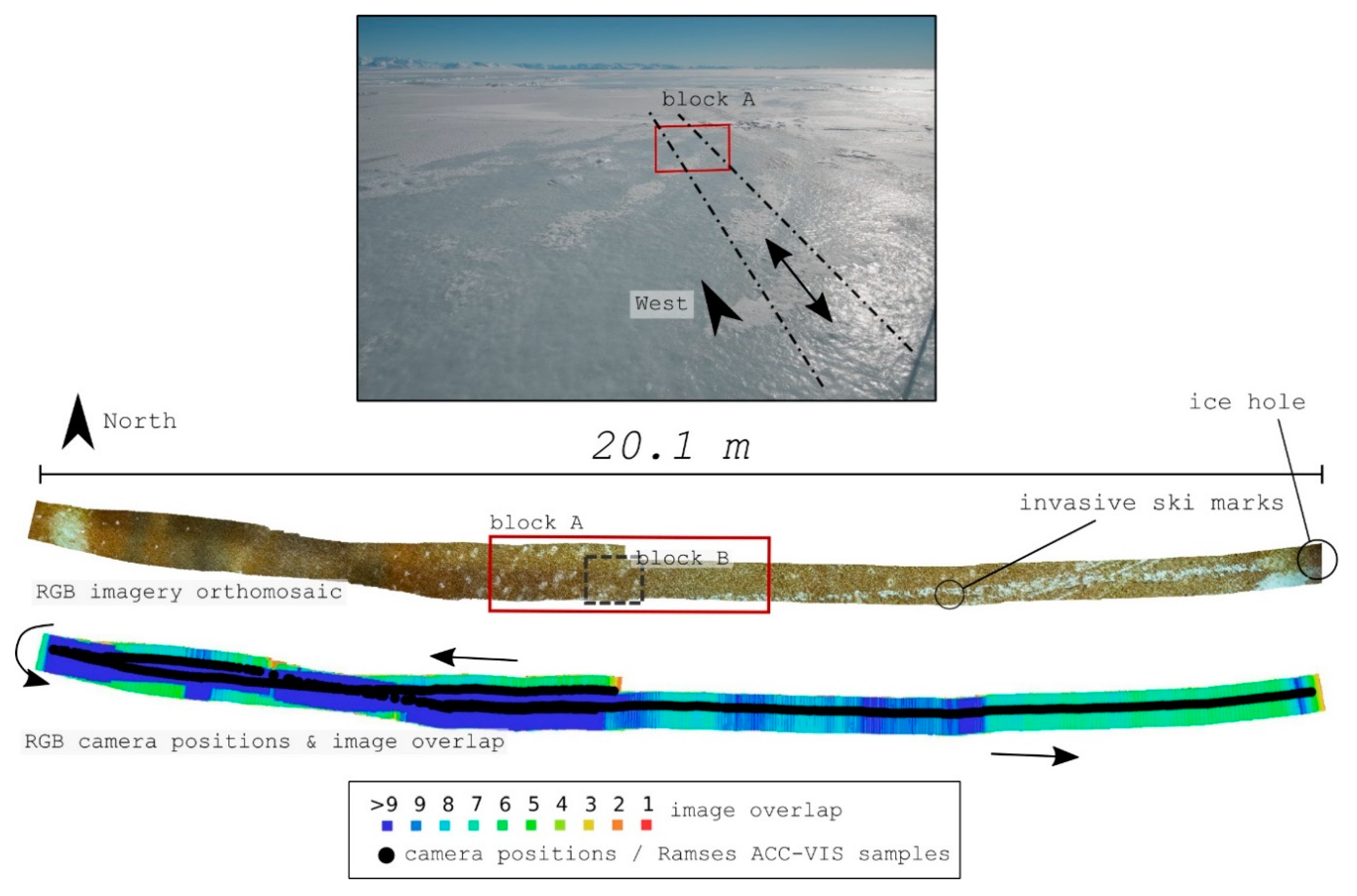
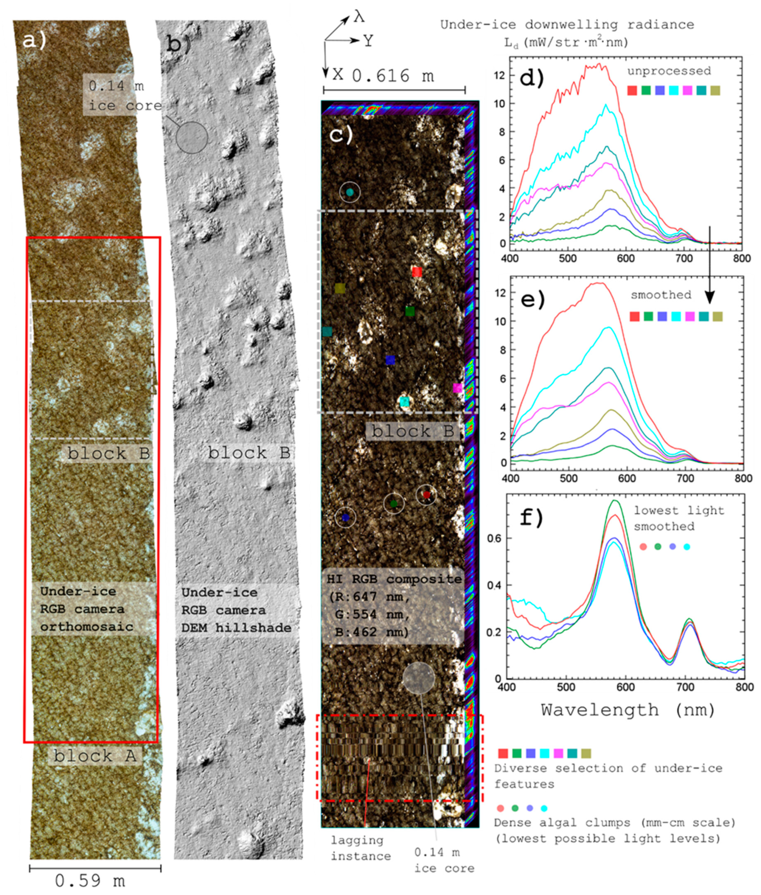
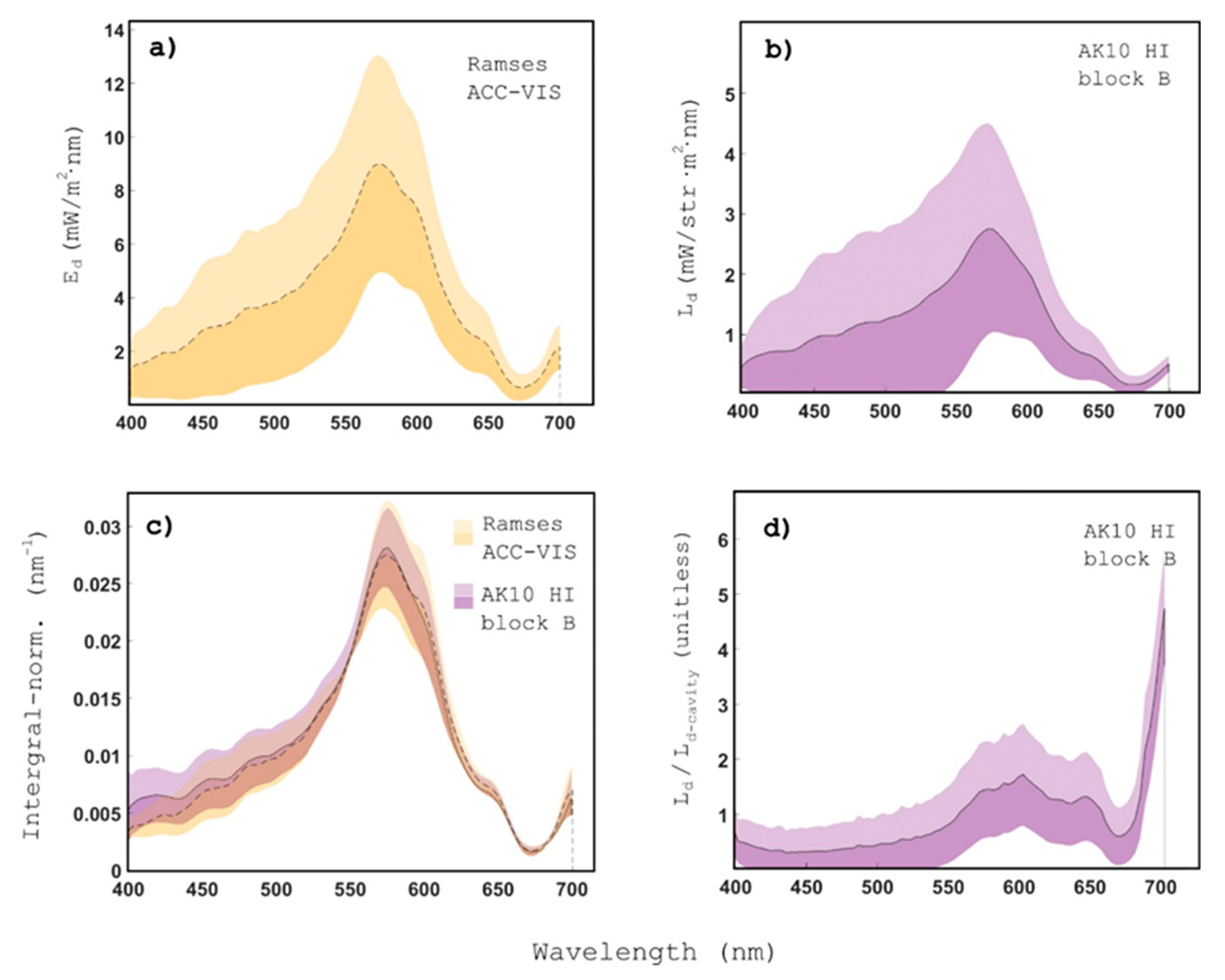
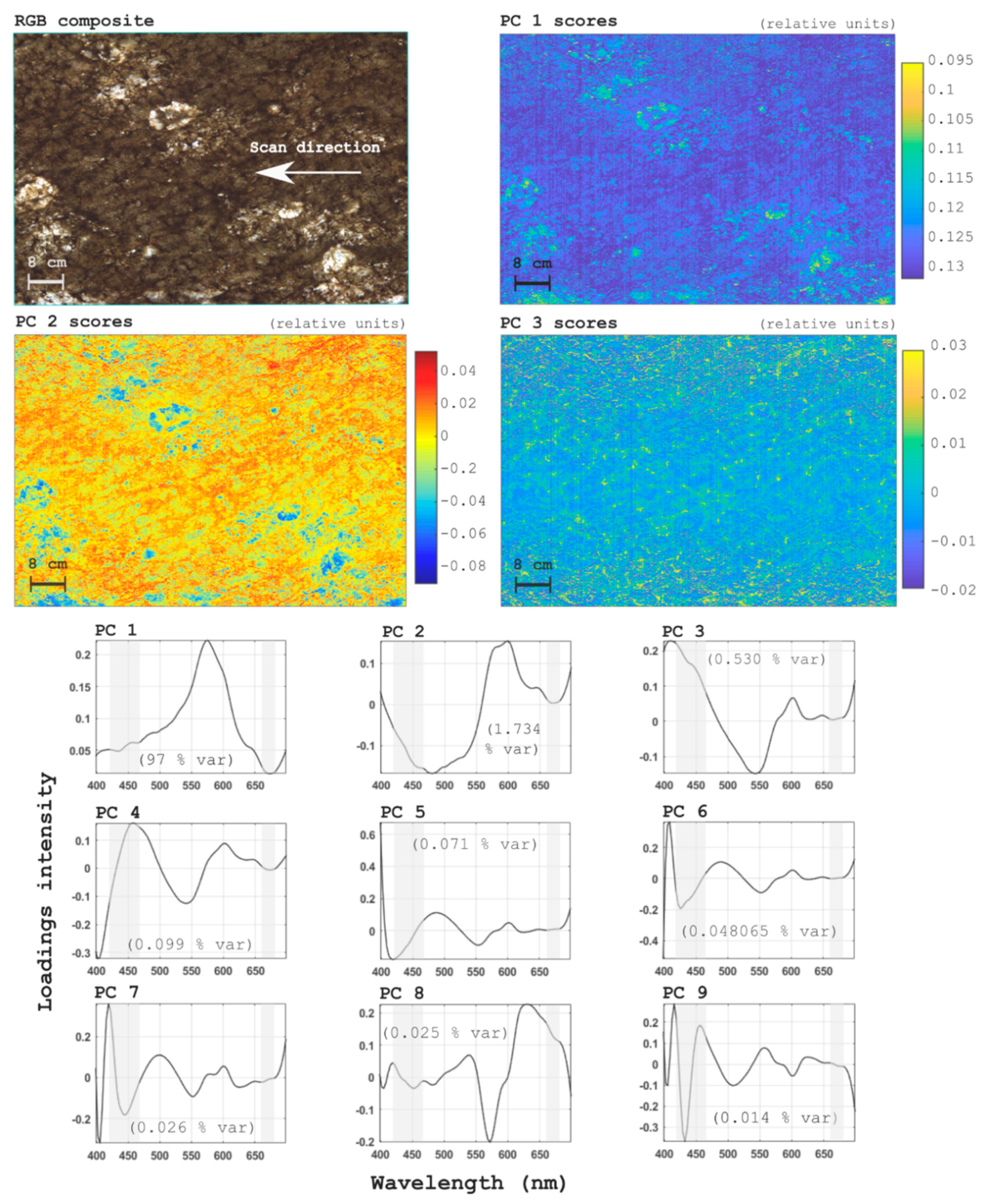
Table 1.
Summary of all optical sensors utilized in the internal and external components of the developed system together with their specifications (top part). The table also includes specifications of other components required to run the system (bottom part). Field of view (FOV)h and FOVv stand for the vertical and horizontal field of view. Underwater FOV is only an ≤ estimate approximation based on simplified theoretical formulas. FWHM refers to full width to half maximum.
| Sensor | Fore-Optics/Lens | Field of View (FOVh/FOVv) | Number of Spatial Pixels | Spectral Range | Spectral Resolution and FWHM |
|---|---|---|---|---|---|
| Specim AISA Kestrel 10 pushbroom sensor | aperture: F/2.4 | 40°/0.0388° in air | 2048 × 1 or 1024 × 1 (binned) | 400–1000 nm | 1.75 / 3.5 / 7 nm/pixel (depending on binning) |
| focal length: 35.375 | ∼29.88°/0.029° underwater | ||||
| Sony a6300 with Samyang AF 35 mm FE | max aperture F/2.8 | 37.2°/25.12° in air | 6000 × 4000 | Visible | RGB |
| focal length: 35 mm | ∼27.5°/18.7° underwater | ||||
| Low Light USB HD cam | focal length: 2.97 mm | 80°/64° in air | 1920 × 1080 | Visible | RGB |
| ∼57.3°/46.6° underwater | |||||
| TriOS Ramses ACC | cosine corrected diffuser | Cosine response | Point sampling | 320–950 nm | 3.3 nm/pixel |
| STS-VIS | CC-3-DA cosine corrected diffuser | Cosine response | Point sampling | 350–800 nm | 3.0 nm/pixel (50 µm slit version) |
| Other components | |||||
| Digital Processing Unit (DPU) | Used to interface and operate all internal sensors/cameras with the surface PC using VNC and has custom electronics from Specim (see Appendix A). Specifications are: Windows 7 Pro, Intel Core i5, 64 bit, 8GB RAM, PIXCI EB1 frame grabber, CameraLink converter, 500 GB HyperX SATA SSD. | ||||
| VN-100 IMU | Measures system attitude used for future geo-rectification of HI imagery (see Appendix A). Operated through the DPU via a Python script. Specifications: 0.5° Static Pitch/Roll, 1.0° Dynamic Pitch/Roll, 5°/hr Gyro In-Run Bias (typ.), 800 Hz IMU Data, ±16 g Accelerometer Range, ±2000°/sec Gyroscope Range, no GPS unit is included in this model. | ||||
| Garmin GPS 18x LVC | Used for above surface GPS lock and time-stamp synchronization (see Appendix A). Specifications: 12-channel GPS receiver tracks, up to 12 satellites, one-pulse-per-second logic-level output with a rising edge aligned to within 1 microsecond of UTC. 1 Hz, output data in NMEA 0183 format. | ||||
| Lumen Subsea Lights (LEDs) | Four units attached as external payload. Intensity manipulated from above surface using a custom build-control. Specifications: Max brightness of 1500 lumens dimmable, beam angle of 135 deg in water and color temperature of 6200 Kelvin. | ||||
© 2019 by the authors. Licensee MDPI, Basel, Switzerland. This article is an open access article distributed under the terms and conditions of the Creative Commons Attribution (CC BY) license (http://creativecommons.org/licenses/by/4.0/).
Share and Cite
MDPI and ACS Style
Cimoli, E.; Meiners, K.M.; Lucieer, A.; Lucieer, V. An Under-Ice Hyperspectral and RGB Imaging System to Capture Fine-Scale Biophysical Properties of Sea Ice. Remote Sens. 2019, 11, 2860. https://doi.org/10.3390/rs11232860
AMA Style
Cimoli E, Meiners KM, Lucieer A, Lucieer V. An Under-Ice Hyperspectral and RGB Imaging System to Capture Fine-Scale Biophysical Properties of Sea Ice. Remote Sensing. 2019; 11(23):2860. https://doi.org/10.3390/rs11232860
Chicago/Turabian StyleCimoli, Emiliano, Klaus M. Meiners, Arko Lucieer, and Vanessa Lucieer. 2019. "An Under-Ice Hyperspectral and RGB Imaging System to Capture Fine-Scale Biophysical Properties of Sea Ice" Remote Sensing 11, no. 23: 2860. https://doi.org/10.3390/rs11232860
Note that from the first issue of 2016, this journal uses article numbers instead of page numbers. See further details here.