Continuous Wavelet Analysis of Leaf Reflectance Improves Classification Accuracy of Mangrove Species
by
 , ,
, ,
Yi Xu
1,3 ,
,
Junjie Wang
2,3,*,
Anquan Xia
4,
Kangyong Zhang
1,3,
Xuanyan Dong
1,3,
Kaipeng Wu
1,3 and
Guofeng Wu
2,3,* 1
College of Civil Engineering, Shenzhen University, Shenzhen 518060, China
2
College of Life Sciences and Oceanography, Shenzhen University, Shenzhen 518060, China
3
Key Laboratory for Geo-Environmental Monitoring of Coastal Zone of the Ministry of Natural Resources & Guangdong Key Laboratory of Urban Informatics & Shenzhen Key Laboratory of Spatial Smart Sensing and Services, Shenzhen University, Shenzhen 518060, China
4
College of Life Sciences, University of Chinese Academy of Sciences, Beijing 100049, China
*
Authors to whom correspondence should be addressed.
Remote Sens. 2019, 11(3), 254; https://doi.org/10.3390/rs11030254
Submission received: 28 December 2018
/
Revised: 18 January 2019
/
Accepted: 24 January 2019
/
Published: 27 January 2019
(This article belongs to the Special Issue Remote Sensing of Mangroves)
Abstract
:Due to continuous degradation of mangrove forests, the accurate monitoring of spatial distribution and species composition of mangroves is essential for restoration, conservation and management of coastal ecosystems. With leaf hyperspectral reflectance, this study aimed to explore the potential of continuous wavelet analysis (CWA) combined with different sample subset partition (stratified random sampling (STRAT), Kennard-Stone sampling algorithm (KS), and sample subset partition based on joint X-Y distances (SPXY)) and feature extraction methods (principal component analysis (PCA), successive projections algorithm (SPA), and vegetation index (VI)) in mangrove species classification. A total of 301 mangrove leaf samples with four species (Avicennia marina, Bruguiera gymnorrhiza, Kandelia obovate and Aegiceras corniculatum) were collected across six different regions. The smoothed reflectance (Smth) and first derivative reflectance (Der) spectra were subjected to CWA using different wavelet scales, and a total of 270 random forest classification models were established and compared. Among the 120 models with CWA of Smth, 88.3% of models increased the overall accuracy (OA) values with an improvement of 0.2–28.6% compared to the model with the Smth spectra; among the 120 models with CWA of Der, 25.8% of models increased the OA values with an improvement of 0.1–11.4% compared to the model with the Der spectra. The model with CWA of Der at the scale of 23 coupling with STRAT and SPA achieved the best classification result (OA = 98.0%), while the best model with Smth and Der alone had OA values of 86.3% and 93.0%, respectively. Moreover, the models using STRAT outperformed those using KS and SPXY, and the models using PCA and SPA had better performances than those using VIs. We have concluded that CWA with suitable scales holds great potential in improving the classification accuracy of mangrove species, and that STRAT combined with the PCA or SPA method is also recommended to improve classification performance. These results may lay the foundation for further studies with UAV-acquired or satellite hyperspectral data, and the encouraging performance of CWA for mangrove species classification can also be extended to other plant species.
1. Introduction
Mangrove forests are communities of diverse salt-tolerant evergreen trees and other plant species in tropical and subtropical intertidal zones, and they provide important ecosystem services such as nutrient cycling, carbon sequestration, and coastal hazard (e.g., shoreline erosion, soil salinization, hurricanes, and tsunamis) mitigation [1,2,3,4]. Due to climate change, natural disasters, and coastal development, the ecological functions of mangrove forests have been continuously degraded for decades [5,6]. The diversity and composition of tree species are key parameters for assessing forest ecosystems [7] and are also particularly essential for understanding their response to environmental change and observing the integrity of endangered ecosystems such as mangroves [8]. Therefore, the accurate classification of mangrove species and in-time monitoring of their spatial distribution are critical for conserving and restoring mangrove forests.
Conventionally, obtaining species information on mangrove forests requires costly, labor-intensive, and time-consuming field investigations, and it is often difficult for investigators to access mangrove forests [9]. Due to rapid, large-scale and cost-effective monitoring capacities, remote sensing techniques have been increasingly adopted to survey and evaluate mangrove resources during the past several decades [10]. Medium-resolution multispectral imagery, such as that from Landsat [11,12], SPOT [13], and Sentinel-2 [8] are often used to map the distribution of mangrove forests at regional or even national or global scales. Due to the advantage of their having superb spatial and textural features and high-resolution multispectral images, satellites such as Quickbird [14], IKONOS [15], Worldview [16,17], and Pléiades-1 [18] have been widely employed to classify mangrove species at landscape or regional scales.
Compared with multi-spectral satellite images with poor spectral information, hyperspectral remote sensing data contain dozens or hundreds of contiguous wavebands with spectral features related to plant functional traits and are found to be more efficient for tree species classification [19]. Leaf [20,21], canopy [21,22,23], satellite (e.g., Hyperion [24,25]), and airborne (e.g., CASI [26], AVIRIS [27,28], and AISA [29]) hyperspectral data have been widely employed in classifying mangrove forests and other forest types (e.g., temperate, subtropical, tropical rainforest, and urban). With rapid advancements in unmanned aerial vehicles (UAV) and self-driving cars, light detection and ranging (LiDAR) techniques have been increasingly utilized in classifying tree species. However, several studies have pointed out that LiDAR alone has not been able to accurately classify tree species, but could be combined with hyperspectral images to further improve classification accuracy [30,31,32]. Therefore, LiDAR-acquired structural parameters are often used as auxiliary information, and the significance of exploring hyperspectral data for plant species classification is still indispensable.
The high dimensionality and multi-collinearity of hyperspectral data may decrease model accuracy in supervised learning processes because the number of spectral wavebands often exceeds the number of model calibration samples [33]. Therefore, additional processing methods are needed for hyperspectral data to resolve the problem of redundant predictors and enhance spectral differences. Considering feature extraction, dimensionality reduction (e.g., principal component analysis (PCA)), waveband selection (e.g., successive projections algorithm (SPA)), and vegetation index (VI) extraction are the three commonly-used strategies in relating sensitive spectral features to the information of plant species [34,35,36]. Moreover, different sample subset partition methods (e.g., stratified random sampling (STRAT), Kennard-Stone sampling algorithm (KS), and sample subset partition based on joint X-Y distances (SPXY)) may cause different classification results [37,38]. However, very few studies have investigated the combination of feature extraction and sample subset partition in the classification of mangrove species.
Continuous wavelet analysis (CWA) is an effective noise reduction method and it can also enhance the details of spectral features of hyperspectral data [39,40,41]. Hence, CWA has been successfully utilized in quantitative remote sensing for retrieving functional traits of plants (e.g., leaf mass per area [42], canopy water content [43], leaf dry matter content and specific leaf area [44]). In contrast, a few studies have applied CWA in improving species classification accuracy in herbaceous wetlands and tropical dry forests [45,46]. However, the advantage of CWA with regards to hyperspectral data is rarely investigated in mangrove species classification.
With the leaf hyperspectral reflectance spectra of four mangrove species samples collected across six regions, this study aimed to explore the potential of CWA combined with different sample subset partition and feature extraction methods in mangrove species classification. The results at the leaf scale may lay the foundation for further studies with UAV- and satellite-based hyperspectral images.
2. Materials and Methods
2.1. Field Sample
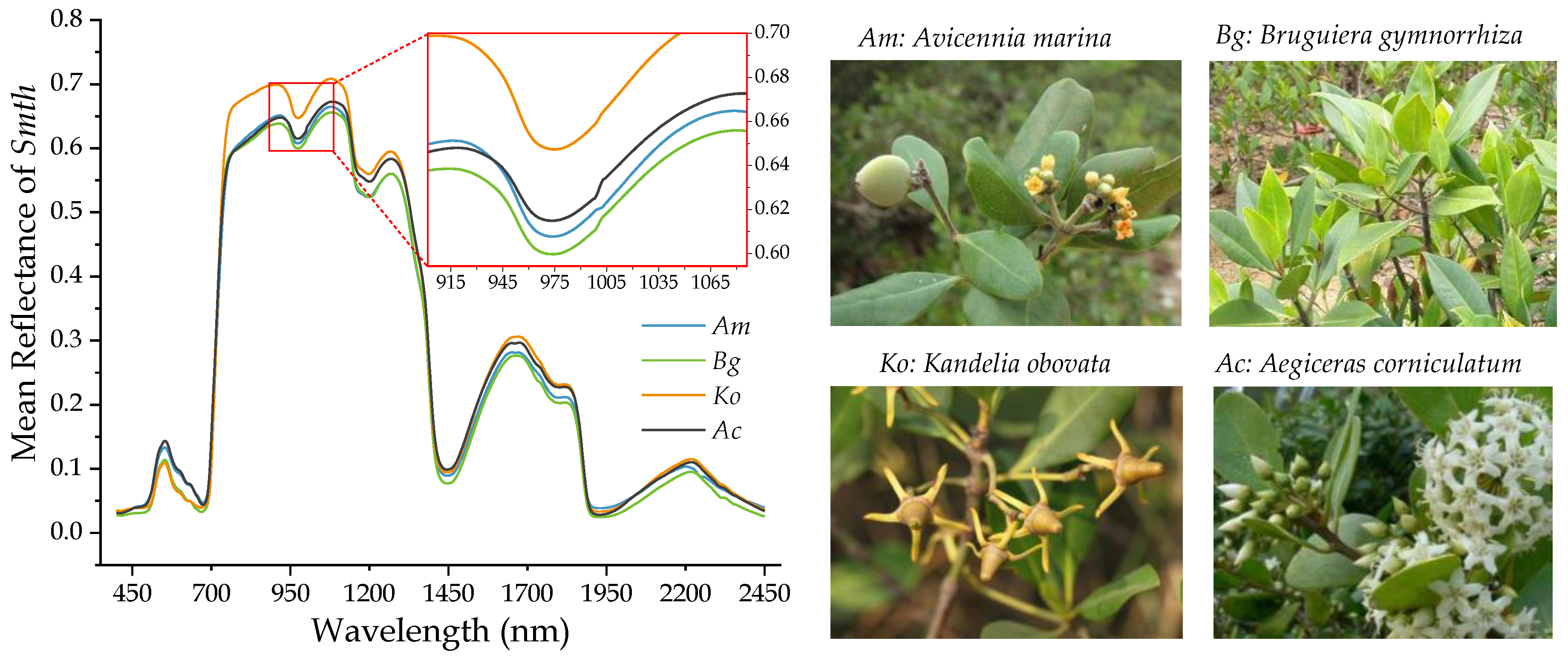
A total of 301 leaf samples of four mangrove species were collected from six sites (Figure 1) in 2017 and 2018 (Table 1), comprising 60 of Avicennia marina, 46 of Bruguiera gymnorrhiza, 81 of Kandelia obovate, and 114 of Aegiceras corniculatum. Each sample was collected from a plot of 10 m × 10 m with a single species, and the center location of each plot was recorded with a global positioning system (GPS) handheld receiver. Moreover, any two plots were at least 30 m apart. For each plot, about 20–30 leaves were picked from the canopy using an extendable trimming pole. To ensure the picked leaves were mature, the leaves between the third and fifth layers from the top were selected [47]. Finally, each sample was instantly sealed in a fresh-keeping bag, kept in a dark box with ice packs, and transported to a nearby laboratory for spectral measurement and chemical analysis.
2.2. Leaf Reflectance Measurement and Spectra Preprocessing
An ASD FieldSpec 4 portable spectroradiometer (Analytical Spectral Devices, Inc., Boulder, CO, USA) was used to measure the leaf spectra reflectance of four mangrove species, and it possesses 2151 wavebands from 350 to 2500 nm with a sampling interval of 1.4 nm in the range of 350–1000 nm and 2 nm in the range of 1000–2500 nm. For each sample, ten leaves were randomly selected in order to measure their spectra with an ASD leaf clip and plant probe; the spectra of each leaf were recorded with ten successive scans and the spectra of ten leaves were averaged as the final reflectance spectra of the target sample.
Due to the systematic noise at two edges of leaf spectrum (350–399 nm and 2451–2500 nm), the leaf reflectance spectra of 301 samples were first reduced to 400–2450nm (Figure 2). To minimize the effects of random noise on model calibration, the remaining spectra were then processed by a Savitzky-Golay smoothing filter with a second order polynomial fit and a window size of seven data points [48]. Finally, the smoothed spectra (hereafter Smth for short) were subjected to first derivative analysis (hereafter Der for short) because this can enhance the peaks and valleys of spectral features [49] and minimize the impact of multiple scatterings of irradiation [50].
2.3. Continuous Wavelet Analysis of Leaf Reflectance
Wavelet analysis is an effective pattern of decomposing the original signal into multiple amplitudes and scales [51,52] and has been widely applied in the field of vegetation remote sensing [41,43,44]. Wavelet analysis is generally implemented in the form of discrete wavelet analysis (DWA) and continuous wavelet analysis (CWA). The former often transforms the most informative part of the input data to avoid redundancy but the decomposed components from DWA are difficult to interpret for waveband-by-waveband analysis [44]. In contrast, CWA generates interpretable signals which directly correspond to original leaf spectra and thus the decomposed signals can reflect the information on plant absorption features [53,54]. Therefore, we employed CWA to explore the details of leaf spectra in the classification of mangrove species.
CWA performs the convolution of reflectance spectrum f (λ) into sets of coefficients with a mother wavelet function at various scales (Equation (1)) [55]. This may be expressed as
where Wf(a,b) (a and b are positive real numbers) is the vector of wavelet coefficients, a and b represent scaling and shifting factors, respectively, indicating the width and position of the wavelet function [56], and is the mother wavelet function.
The shape of the leaf reflectance spectrum is similar to a Gaussian or quasi-Gaussian function, or a composition of several Gaussian functions [57]. Based on the suggestion of Torrence et al. [58], the second order derivative of Gaussian (namely the ‘Mexican Hat’, “mexh”) was chosen as the mother wavelet function (Figure 3). The ”mexh” function has symmetry and its mean power is zero [59]. Moreover, the ”mexh” function has an infinite support width of (–5s, 5s) () and its effective basic support range is (–5, 5) [60].
To decrease intensive computation, according to the suggestion of Cheng et al. [61], CWA was only performed at dyadic scales instead of all possible scales. Moreover, the 2051 wavebands (400–2450nm) available in this study made the dyadic scale less than 210 = 1024. Based on the suggestion of Cheng et al. [42] and the preliminary experiments of mangrove species classification, the eight scales (20, 21,… , 27) were chosen for CWA of Smth and Der (or named “wavelet power spectra of Smth and Der”), and CWA was implemented with the wavelet packets of MATLAB R2018a.
2.4. Establishment of Mangrove Species Classification Model
To examine the impact of different sample subset partition and feature extraction methods on the performance of mangrove species classification, three commonly-used subset partition methods (STRAT, KS, and SPXY) and feature selection methods (PCA, SPA, and VI) were tested and compared, respectively. Random forests (RF), a prevalent and successful machine learning method, was chosen as the classification model in this study.
According to the suggestion of Roth et al. [62], to ensure the modeling and prediction sets contained samples of each species, the original dataset (301 samples) was first divided into two sets with STRAT, using 70% (211) of samples for modeling and 30% (90) of samples for prediction (Figure 4). The reason for this partition strategy of selecting the prediction sets was that the KS and SPXY algorithms selected sample subsets based on the Euclidean distances of x-space or x and y space which resulted in an unbalanced prediction sample size of four species. Afterwards, the modeling set was divided into two sets, with 70% (148 samples) being used as a calibration set to construct species classification models and the remaining samples (the validation set) being eliminated due to the aforementioned influence of KS and SPXY. Each process of sample subset partitioning was repeated 50 times to ensure the reliability of the classification results [63].
A total of 270 (18 × 3 × 5) models were constructed, considering 18 types of spectra (Smth, Der, Smth + CWA (eight scales), and Der + CWA (eight scales)) in conjunction with three sample subset partition (STRAT, KS, and SPXY) and five feature extraction methods (PCA, SPA, and three VIs). To simply and clearly present the 270 models, CWA of Smth and Der were expressed in Smth_scale and Der_scale (scale = 1, 2, 4, 8, 16, 32, 64, 128) and the combination of sample subset partition and feature extraction was represented in STRAT_PCA, which indicated the sample subset was partitioned by STRAT and the feature was in the meantime extracted by PCA.
2.4.1. Sample Subset Partition
Compared with simple random sampling (SRS), STRAT can select more representative samples and is especially suitable for remote-based plant species classification [28]. The KS algorithm calculates the Euclidean distances within different samples along the independent variable (x) space using a stepwise procedure; two samples with the farthest Euclidean distance are first selected and the next sample selected is the farthest one from the first two samples [64]. SPXY improves on the KS algorithm [65] by extending the Euclidean distance calculation with both independent and dependent variables. For details of KS and SPXY refer to Galvao et al. [65]. The three aforementioned sample subset partition methods were implemented with MATLAB R2018a.
2.4.2. Feature Extraction
PCA is a typical dimensionality reduction method which is widely applied in hyperspectral image analysis [34,66]. In this study, spectra (Smth, Der, Smth + CWA (eight scales), and Der + CWA (eight scales)) were subjected to PCA using a pca() function in MATLAB R2018a, and the leading several principal components were chosen based on the eigenvalues-greater-than-one rule to calibrate the model [67]. In addition, we added up the percentages of total variance explained by the selected principal components for each spectrum (Table 2).
SPA is a forward variable selection algorithm which begins with a waveband, merges a new one during each iteration, and applies projection operators in a vector space until meeting a specified number of wavebands [68]. The advantage of SPA lies in its deterministic search process with good robustness and reproducible results. The ratio of the number of selected wavebands to the total number of training samples is 0.15–0.2 to avoid over-fitting problems [69]. Gross, et al. [45] discovered that model performance with less than 20 features was relatively stable, and extra features evidently increased computation time. Hence, we set the parameter m_max (maximum number of variables) of the spa() function as 20. The process was implemented with SPA code (www.ele.ita.br/~kawakami/spa) in MATLAB R2018a.
VIs are generally derived from two or three wavebands to detect the differences of plant physiology and biochemistry [69]. There are many forms of VIs based on different mathematical rules, and those commonly-used are normalized difference vegetation index (NDVI = ()/()) [70], ratio vegetation index (RVI = /) [71] and three bands vegetation index (TBVI = /()) [72]. The wavebands selected by SPA from spectra (Smth, Der, Smth + CWA (eight scales), and Der + CWA (eight scales)) were then used to construct the three forms of VI. The selected wavebands generated n × (n − 1) (n being the number of wavebands selected by SPA) combinations of all possible NDVIs and RVIs, and n × (n − 1) × (n − 2)/2 combinations of TBVIs. The computations were carried out in MATLAB R2018a.
2.4.3. Random Forests Classification
The RF algorithm introduces decision trees, the bagging (bootstrapping aggregation) sampling method and internal cross-validation into K binary Classification and Regression Trees (CART) trees, and can effectively overcome the over-fitting problem of machine learning [73,74,75]. Hundreds of decision tree models are constructed by RF and the randomized subsets of target data and variables are utilized for building each tree [76]. These classification trees are then used to determine the correct classification by majority voting [77]. There are two main tuning parameters (ntree and mtry) needed in a RF model, and both of them are kept at the default values because researchers have reported that the default values and the empirical criteria generally produce acceptable results [74,78]. The RF was performed with RF code (https://code.google.com/archive/p/randomforest-matlab/downloads) in MATLAB R2018a.
2.5. Evaluation of Classification Model Performance
Overall accuracy (OA) (Equation (2)), producer’s accuracy (PA) (Equation (3)) and user’s accuracy (UA) (Equation (4)) were employed to evaluate the performance of each classification model. Furthermore, the allocation disagreement (AD) (Equation (5)) and quantity disagreement (QD) (Equation (6)) were adopted rather than Kappa, since Kappa neglects the assessment of off-diagonal elements [79] which is highly relevant to OA [63]. For specific descriptions and explanations of AD and QD refer to Jr et al. [80] and Nurmemet et al. [81]. The larger the values of OA, PA, or UA, the better the model performance; however, the larger the value of AD or QD, the poorer the model performance. These aforementioned methods may be expressed as
![Remotesensing 11 00254 i001]() where is a error matrix (Equation (7)), and i is the row/column number of relevant species; represents the sum of the ith row of the error matrix, reflecting the total number of the samples in ith species divided into the ith species and the other three species; represents the sum of the ith column of the error matrix, reflecting the total number of samples divided into ith species; , the ith diagonal element of error matrix, indicates the number of species correctly classified; and n is the sample size of prediction sets.
where is a error matrix (Equation (7)), and i is the row/column number of relevant species; represents the sum of the ith row of the error matrix, reflecting the total number of the samples in ith species divided into the ith species and the other three species; represents the sum of the ith column of the error matrix, reflecting the total number of samples divided into ith species; , the ith diagonal element of error matrix, indicates the number of species correctly classified; and n is the sample size of prediction sets.

3. Results
3.1. Mean Reflectance and Wavelet Power Spectra of Mangrove Leaf
Taking Am (Avicennia marina) for instance (the cases of other species can be found in Figure S1-1,S1-2 (see supplementary material Figure S1), the mean reflectance and wavelet power spectra of Smth/Der with eight scales are illustrated in Figure 5. The mean reflectance spectra of Smth only had 10 peaks and 10 troughs (Figure 5a), while 52 peaks and 53 troughs were observed for the first derivative spectra (Figure 5b). Compared with the spectra of Smth/Der, the number of peaks and troughs for the wavelet power spectra of Smth/Der (scale = 1, 2, and 4) experienced a substantial increase with much more detailed spectral features; however, the wavelet power spectra with the scales of 32–128 had less information of spectral features than the spectra of Smth/Der. The other three species (Figure S1-1,S1-2 (Figure S1)) also experienced the same condition with first derivative and wavelet power spectra (scale = 1, 2, and 4), which enhanced the differences of spectral wavebands and improved the details of spectral features.
3.2. Performance of Classification Models with Reflectance, Derivative and Wavelet Power Spectra
To explore the advantage of CWA on mangrove species classification, the OAs, Ads, and QDs of the 270 models with reflectance, derivative, and wavelet power spectra were summarized and compared (Table 3). Regardless of the effect of sample subset partition and feature extraction, the models with CWA of Smth spectra at the scales of 21-26 (also Smth_2, Smth_4, Smth_8, Smth_16, Smth_32, and Smth_64) and CWA of Der spectra at the scale of 23 and 24 (also Der_8 and Der_16) had higher mean OAs and lower mean QDs than those with Smth/Der spectra; the Der spectra achieved much better classification performance than the Smth spectra. In addition, among the 120 models with the wavelet power spectra of Smth, 88.3% of models increased the OA values with an improvement of 0.2–28.6% compared to the model with the Smth spectra, and among the 120 models with the wavelet power spectra of Der, 25.8% of models increased OA values, with an improvement of 0.1–11.4% compared to the model with the Der spectra (Table S1—OA comparison).
Among the 270 models, the models with Smth_4 and Der_8 spectra had the highest mean classification accuracies; however, the models with CWA of Smth spectra at the scale of 128 and CWA of Der spectra at the scale of 1 had the poorest classification performances. The two models with CWA of Smth/Der spectra at the scale of 8 held the best classification accuracies, with OA reaching 97.6% and 98.0%, respectively.
3.3. Performance of Models with Different Sample Subset Partition Methods
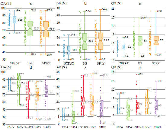
To explore the effect of different sample subset partition methods on the model performance of mangrove species classification, the OAs, ADs and QDs of the 270 models using the STRAT, KS and SPXY methods were compared (Figure 6). The models using the STRAT method (mean OA = 84.5%, mean AD = 10.8%, and mean QD = 4.8%) achieved better classification results than those using the KS (mean OA = 72.7%, mean AD = 20.4%, and mean QD = 6.9%) and SPXY (mean OA = 71.7%, mean AD = 21.3%, and mean QD = 7.0%) methods. Moreover, the standard deviation of the OAs, ADs, and QDs using the STRAT method (SD = 6.7%, 5.9%, and 1.2%, respectively) were much smaller than those using the KS (SD = 13.1%, 11.3%, and 2.4%, respectively) and SPXY (SD = 13.7%, 11.9%, and 2.6%, respectively) methods. In addition, the lowest accuracies of models using these three methods (OA = 66.2% for STRAT, OA = 38.0% for KS, and OA = 36.9% for SPXY) occurred with the wavelet power spectra of Der_1.
3.4. Performance of Classification Models with Different Feature Extraction Methods
To explore the effect of different feature extraction methods on the model performance of mangrove species classification, the OAs, ADs, and QDs of the 270 models using PCA, SPA, and three VIs (NDVI, RVI, and TBVI) were compared (Figure 7). The ranking order of the mean OA values was PCA > SPA > TBVI > NDVI > RVI, while PCA < SPA < TBVI < NDVI < RVI for the mean AD values and SPA < PCA < TBVI < NVDI < RVI for the mean QD values. The models using PCA had lower standard deviation values of the OAs, ADs, and QDs (SD = 4.6%, 3.5%, and 1.5%, respectively) than those with the other four methods. Moreover, the model using SPA combined with the STRAT method and the wavelet power spectra of Der_8 achieved the highest OA value of 98.0% among the 270 models.
Among the three VIs, there were no significant differences between NDVI and RVI in mangrove species classification considering the mean or the SD values of OAs, Ads, and QDs; however, both provided lower classification results than TBVI (mean OA = 72.7%, mean AD = 17.2%, and mean QD = 6.6%). Notably, the model using TBVI (the three wavebands were 730, 1680, and 1735 nm) combined with the STRAT method and the wavelet power spectra of Smth_4 held the highest OA value of 93.6% among the models using VIs, which was higher than the best result of the models using PCA (Figure 7a).
To explore which waveband or spectral range was sensitive to mangrove species classification, the wavebands which were frequently selected (with ratios of the frequency of the specific waveband to the number of all the wavebands selected by SPA greater than 0.01) by SPA (54 models, 714 selected wavebands in total) and VIs (54 × 3 = 162 models, 378 selected wavebands in total) were compiled (Table 4). The selected bands mostly lie in the range of 680–780 nm (red edge region), 1650–1950 nm, and 2200–2450 nm.
4. Discussion
4.1. Continuous Wavelet Analysis for Mangrove Species Classification
With leaf hyperspectral reflectance, we have explored the potential of CWA combined with different sample subset partition and feature extraction methods in mangrove species classification, and study results have demonstrated that CWA of Smth and Der spectra with suitable wavelet scales could greatly improve the classification accuracy compared to Smth or Der spectra alone (Table 3). Notably, although low-scale (e.g., scale = 1) wavelet coefficients were able to discover numerous details from leaf spectra (Figure 5), the results were unsatisfactory (mean OA: 63.6%); the high-scale (e.g., scale = 128) wavelet coefficients also corresponded to poorer performance of classification (mean OA: 69.3%). Such unsuccessful results may be explained by the fact that the low or high scales of wavelet power spectra have noise, or insensitive or less detailed spectral information related to leaf structure and biochemical components [41,44]. In addition, both the derivative analysis and CWA can enhance the differences of spectral wavebands; however, their combination did not improve the accuracy at the scale of 21 or 22, suggesting that the details of the original spectra could be largely preserved by derivative analysis or CWA alone. Such inference could also be supported by the result of Der spectra performing much better than Smth spectra. In general, low-scale wavelet coefficients are adept at detecting the characteristics of narrow absorption features of leaves but high-scale coefficients are expert in determining the overall spectral shape of leaf reflectance spectra [44]. Therefore, it is of crucial importance to determine the suitable wavelet scale when reflectance or derivative spectra are subjected to CWA.
Considering relevant studies using CWA on hyperspectral data at the leaf level, many studies have reported that the optimal scale of CWA in plant disease detection and biochemical component estimation lies between 22 and 25. For instance, Shi et al. [41] selected wavelet features at the scales of 22, 24 and 25 to study rust infestation; Zhang et al. [23] identified disease sensitive wavelet features at the scales of 22~4; Li et al. [82] found the performance of scale 23 was the best for extracting the red edge position from leave reflectance; and 24 was specified as the optimal scale for estimating leaf water content and leaf dry matter content by Cheng et al. [54] and Cheng et al. [42], respectively. Therefore, the optimal continuous wavelet scales between 22 and 25 are still required to be investigated in future studies.
Previous studies have reported the classification of mangrove species without CWA. For instance, Zhang et al. [23] coupled laboratory leaf hyperspectral reflectance with mangrove health conditions, acquiring an OA around 90%. In terms of other plant species classification without CWA, Shen et al. [34] combined airborne hyperspectral images with LiDAR to classify tree species of subtropical forests and their best OA reached around 91.5%. Our study has revealed the advantage of CWA in mangrove species classification, and the fact that it is promising to employ CWA to further improve the accuracy of plant species classification with drone or satellite-based hyperspectral data.
4.2. Impact of Sample Subset Partition and Feature Extraction on Classification Accuracy
Our results have demonstrated that the selection of sample subset partition and feature extraction methods play an important role in improving the accuracies of mangrove species. Generally, the models using STRAT method exhibited more stable and higher classification accuracies than those using KS and SPXY methods. To our knowledge, very few studies have applied SPXY in the sample partition for plant species classification, and comparisons among SRS, KS and SPXY have been performed in quantitative models to determine the asiaticoside content in centella total glucosides [83]. However, Zhan et al. [83] have concluded that the model using SPXY achieves the highest prediction accuracy which was contrary to our results. Such disagreement may be related to differences in species, models or the statistical distribution of dependent variables. Moreover, the sample subset partitioned by KS and SPXY cannot ensure the equal number of samples for each species. Hence, it is recommended to employ STRAT method in plant species classification.
Regarding the feature extraction method, the performances of the models using PCA and SPA were better than those using VIs, which could be explained by the fact that VIs had less spectra features with only two or three wavebands. This inference could be supported by the results of the models using TBVI, because TBVI has only one more waveband than NDVI and RVI, but the OAs of the models using TBVI were higher than those using NDVI and RVI. Although the models using SPA had slightly lower mean classification accuracies than those using PCA (Figure 7), the former models could have better waveband explanation and the model using SPA coupled with CWA of Der at the scale of 8 and STRAT had the best classification result among the 270 models. Guzmán Q et al. [39] recently solely applied PCA to realize data reduction and successfully discriminated liana and tree leaves from a neotropical dry forest. Hence, it is difficult to determine whether PCA or SPA is more suitable for mangrove species classification, and both methods still require investigation with other plant species or other forms of hyperspectral data (satellite-based or UAV-acquired).
This study has only focused on wavebands selected by SPA and VIs and many of the selected wavebands lie in the red edge region (680–780 nm) (Table 4). Red edge species are sensitive to vegetation chlorophyll, stress, dynamics, and nitrogen accumulation [84,85]. Moreover, the selected wavebands located around 1885 and 2245 nm are related to foliar starch [86]. The selected wavebands within 1600–1750 nm might be associated with complex biochemical properties, such as salt, sugar, water, protein, oil, lignin, starch, and cellulose, as well as leaf structure [10]; and the wavebands in the range of 1900–1950 nm and around 1400 nm are strongly affected by water absorption [86]. The hyperspectral data alone could explore the sensitive spectral information related to mangrove species classification, and the integration of spectral information and supplementary data (e.g., biochemical components, soil property, and geomorphology) might help to further understand the mechanism of mangrove species composition and extend the classification model to other study sites.
4.3. Taxonomically Comparing the Accuracy of Mangrove Species Classification
Some studies mention that the spectral differences of plants within different taxonomic levels are significant [87,88,89]. Kiang et al. [88] found that the spectral differences within higher taxonomic levels were more pronounced than those within lower taxonomic levels. Hence, we compiled detailed taxonomical information (Figure S1-3 (Figure S1)) (source: Flora Reipublicae Popularis Sinicae, frps.iplant.cn) on four mangrove species.
Bg and Ko belong to the same family, while Am and Ac are classified into different orders. In most cases, the PAs and UAs of Bg and Ko are lower than Am and Ac (Figure S1-5 (Figure S1)). Moreover, we found that the majority of the error-classifying of Bg and Ko samples were classified into Ko and Bg, respectively, which may be explained by the fact that the shape, size and thickness of their leaves are similar and their biochemical components are approximate (leaf water content (Ko: 70.93% (SD = 2.82%); Bg: 68.27% (SD = 2.67%)); chlorophyll (metered by SPAD-502, Ko: 68.6 (SD = 5.18); Bg: 70.1 (SD = 3.89)). In general, we can infer that it is still a challenge to use hyperspectral data alone to accurately discriminate between taxonomically similar species, and supplementary information such as canopy structure, leaf area index, and leaf biochemical components may be incorporated into the classification model to improve the accuracies of species discrimination.
5. Conclusions
With leaf hyperspectral data, we have explored the potential of CWA coupled with different sample subset partition and feature extraction methods in mangrove species classification. The following conclusions may be drawn:
- 1)
- Regardless of the effect of sample subset partition and feature extraction methods on the performance of mangrove species classification, CWA with suitable scales has great potential to improve the classification accuracy.
- 2)
- The STRAT method combined with PCA or SPA methods is recommended to improve classification performance.
- 3)
- Compared with the original reflectance spectra, the derivative spectra can significantly improve the classification accuracy.
The leaf-level results can lay the foundation for the next step in-depth study of mangrove species classification with UAV-acquired or satellite hyperspectral data, contributing to understanding large-scale species composition and further effectively protect and manage mangrove forests. Moreover, the encouraging performance of CWA can also be extended to other plant species such as forest and crop. Further, eco-environment factors (e.g., elevation, soil property, leaf biochemical components, and canopy structure) are required to investigate their effects on the performance of mangrove species classification in future studies.
Supplementary Materials
The following are available online at https://www.mdpi.com/2072-4292/11/3/254/s1, Figure S1: Supplementary Figures, Table S1: Statistics.
Author Contributions
Y.X., J.W., A.X., K.Z., X.D., and K.W. conducted the in-situ surveys; Y.X., J.W., and A.X. performed the hyperspectral observations; Y.X. and J.W. conceived and designed the experiments, and analyzed the results; Y.X., J.W. and G.W. wrote and revised the manuscript. G.W. and J.W. provided useful suggestions to the manuscript.
Funding
This research was funded by the National Key R&D Program of China (No. 2017YFC0506200), National Natural Science Foundation of China (No. 41601362), the Basic Research Program of Shenzhen Science and Technology Innovation Committee (No. JCYJ20151117105543692), and the Scientific Research Foundation for Newly High-End Talents of Shenzhen University.
Acknowledgments
The authors would like to thank all the anonymous reviewers and the assistant editor (Joss Chen) for their constructive comments and suggestions on this manuscript.
Conflicts of Interest
The authors declare no conflict of interest.
References
- Tam, N.F.Y.; Wong, Y.S. Mangrove soils in removing pollutants from municipal wastewater of different salinities. J. Environ. Qual. 1999, 28, 556–564. [Google Scholar] [CrossRef]
- Murdiyarso, D.; Purbopuspito, J.; Kauffman, J.B.; Warren, M.W.; Sasmito, S.D.; Donato, D.C.; Manuri, S.; Krisnawati, H.; Taberima, S.; Kurnianto, S. The potential of Indonesian mangrove forests for global climate change mitigation. Nat. Clim. Chang. 2015, 5, 1089–1092. [Google Scholar] [CrossRef]
- Mao, L.M.; Zhang, Y.L.; Bi, H. Modern pollen deposits in coastal mangrove swamps from northern Hainan Island, China. J. Coast. Res. 2006, 22, 1423. [Google Scholar] [CrossRef]
- Lugo, A.E.; Snedaker, S.C. The ecology of mangroves. Annu. Rev. Ecol. Syst. 1974, 5, 39–64. [Google Scholar] [CrossRef]
- Jia, M.M.; Liu, M.Y.; Wang, Z.M.; Mao, D.H.; Ren, C.Y.; Cui, H.S. Evaluating the Effectiveness of Conservation on Mangroves: A Remote Sensing-Based Comparison for Two Adjacent Protected Areas in Shenzhen and Hong Kong, China. Remote Sens. 2016, 8, 627. [Google Scholar] [CrossRef]
- Chakravortty, S.; Li, J.; Plaza, A. A Technique for Subpixel Analysis of Dynamic Mangrove Ecosystems with Time-Series Hyperspectral Image Data. IEEE J. Sel. Top. Appl. Earth Obs. Remote Sens. 2018, 11, 1244–1252. [Google Scholar] [CrossRef]
- Richter, R.; Reu, B.; Wirth, C.; Doktor, D.; Vohland, M. The use of airborne hyperspectral data for tree species classification in a species-rich Central European forest area. Int. J. Appl. Earth Obs. Geoinf. 2016, 52, 464–474. [Google Scholar] [CrossRef]
- Wang, D.; Wan, B.; Qiu, P.; Su, Y.; Guo, Q.; Wang, R.; Sun, F.; Wu, X. Evaluating the Performance of Sentinel-2, Landsat 8 and Pléiades-1 in Mapping Mangrove Extent and Species. Remote Sens. 2018, 10, 1468. [Google Scholar] [CrossRef]
- Cao, J.J.; Leng, W.C.; Liu, K.; Liu, L.; He, Z.; Zhu, Y.H. Object-Based Mangrove Species Classification Using Unmanned Aerial Vehicle Hyperspectral Images and Digital Surface Models. Remote Sens. 2018, 10, 89. [Google Scholar] [CrossRef]
- Kuenzer, C.; Bluemel, A.; Gebhardt, S.; Quoc, T.V.; Dech, S. Remote Sensing of Mangrove Ecosystems: A Review. Remote Sens. 2011, 3, 878–928. [Google Scholar] [CrossRef] [Green Version]
- Bullock, E.L.; Fagherazzi, S.; Nardin, W.; Vo-Luong, P.; Nguyen, P.; Woodcock, C.E. Temporal patterns in species zonation in a mangrove forest in the Mekong Delta, Vietnam, using a time series of Landsat imagery. Cont. Shelf Res. 2017, 147, 144–154. [Google Scholar] [CrossRef]
- Heumann, B.W. Satellite remote sensing of mangrove forests: Recent advances and future opportunities. Prog. Phys. Geogr. 2011, 35, 87–108. [Google Scholar] [CrossRef]
- Hauser, L.T.; Vu, G.N.; Nguyen, B.A.; Dade, E.; Nguyen, H.M.; Nguyen, T.T.Q.; Le, T.Q.; Vu, L.H.; Tong, A.T.H.; Pham, H.V. Uncovering the spatio-temporal dynamics of land cover change and fragmentation of mangroves in the Ca Mau peninsula, Vietnam using multi-temporal SPOT satellite imagery (2004–2013). Appl. Geogr. 2017, 86, 197–207. [Google Scholar] [CrossRef]
- Neukermans, G.; Dahdouh-Guebas, F.; Kairo, J.G.; Koedam, N. Mangrove species and stand mapping in GAzi bay (Kenya) using Quickbird satellite imagery. J. Spat. Sci. 2008, 53, 75–86. [Google Scholar] [CrossRef]
- Xin, H.; Liangpei, Z.; Le, W. Evaluation of Morphological Texture Features for Mangrove Forest Mapping and Species Discrimination Using Multispectral IKONOS Imagery. IEEE Geosci. Remote Sens. Lett. 2009, 6, 393–397. [Google Scholar] [CrossRef] [Green Version]
- Heenkenda, M.K.; Joyce, K.E.; Maier, S.W.; Bartolo, R. Mangrove Species Identification: Comparing WorldView-2 with Aerial Photographs. Remote Sens. 2014, 6, 6064–6088. [Google Scholar] [CrossRef] [Green Version]
- Wang, T.; Zhang, H.; Lin, H.; Fang, C. Textural–spectral feature-based species classification of mangroves in Mai Po Nature Reserve from Worldview-3 imagery. Remote Sens. 2015, 8, 24. [Google Scholar] [CrossRef]
- Wang, D.; Wan, B.; Qiu, P.; Su, Y.; Guo, Q.; Wu, X. Artificial Mangrove Species Mapping Using Pléiades-1: An Evaluation of Pixel-Based and Object-Based Classifications with Selected Machine Learning Algorithms. Remote Sens. 2018, 10, 294. [Google Scholar] [CrossRef]
- Govender, M.; Chetty, K.; Naiken, V.; Bulcock, H. A comparison of satellite hyperspectral and multispectral remote sensing imagery for improved classification and mapping of vegetation. Water SA 2008, 34, 147–154. [Google Scholar]
- Wang, L.; Sousa, W.P. Distinguishing mangrove species with laboratory measurements of hyperspectral leaf reflectance. Int. J. Remote Sens. 2009, 30, 1267–1281. [Google Scholar] [CrossRef]
- Prasad, K.A.; Gnanappazham, L. Multiple statistical approaches for the discrimination of mangrove species ofRhizophoraceaeusing transformed field and laboratory hyperspectral data. Geocarto Int. 2015, 31, 891–912. [Google Scholar] [CrossRef]
- Manjunath, K.R.; Kumar, T.; Kundu, N.; Panigrahy, S. Discrimination of mangrove species and mudflat classes using in situ hyperspectral data: A case study of Indian Sundarbans. GISci. Remote Sens. 2013, 50, 400–417. [Google Scholar] [CrossRef]
- Zhang, C.H.; Kovacs, J.M.; Liu, Y.L.; Flores-Verdugo, F.; Flores-de-Santiago, F. Separating Mangrove Species and Conditions Using Laboratory Hyperspectral Data: A Case Study of a Degraded Mangrove Forest of the Mexican Pacific. Remote Sens. 2014, 6, 11673–11688. [Google Scholar] [CrossRef] [Green Version]
- Jia, M.; Zhang, Y.; Wang, Z.; Song, K.; Ren, C. Mapping the distribution of mangrove species in the Core Zone of Mai Po Marshes Nature Reserve, Hong Kong, using hyperspectral data and high-resolution data. Int. J. Appl. Earth Obs. Geoinf. 2014, 33, 226–231. [Google Scholar] [CrossRef]
- Wong, F.K.K.; Fung, T. Combining EO-1 Hyperion and Envisat ASAR data for mangrove species classification in Mai Po Ramsar Site, Hong Kong. Int. J. Remote Sens. 2014, 35, 7828–7856. [Google Scholar] [CrossRef]
- Held, A.; Ticehurst, C.; Lymburner, L.; Williams, N. High resolution mapping of tropical mangrove ecosystems using hyperspectral and radar remote sensing. Int. J. Remote Sens. 2010, 24, 2739–2759. [Google Scholar] [CrossRef]
- Hirano, A.; Madden, M.; Welch, R. Hyperspectral image data for mapping wetland vegetation. Wetlands 2003, 23, 436–448. [Google Scholar] [CrossRef]
- Kamal, M.; Phinn, S. Hyperspectral Data for Mangrove Species Mapping: A Comparison of Pixel-Based and Object-Based Approach. Remote Sens. 2011, 3, 2222–2242. [Google Scholar] [CrossRef] [Green Version]
- Vaglio Laurin, G.; Puletti, N.; Hawthorne, W.; Liesenberg, V.; Corona, P.; Papale, D.; Chen, Q.; Valentini, R. Discrimination of tropical forest types, dominant species, and mapping of functional guilds by hyperspectral and simulated multispectral Sentinel-2 data. Remote Sens. Environ. 2016, 176, 163–176. [Google Scholar] [CrossRef] [Green Version]
- Liu, L.X.; Coops, N.C.; Aven, N.W.; Pang, Y. Mapping urban tree species using integrated airborne hyperspectral and LiDAR remote sensing data. Remote Sens. Environ. 2017, 200, 170–182. [Google Scholar] [CrossRef]
- Sankey, T.; Donager, J.; McVay, J.; Sankey, J.B. UAV lidar and hyperspectral fusion for forest monitoring in the southwestern USA. Remote Sens. Environ. 2017, 195, 30–43. [Google Scholar] [CrossRef]
- Sankey, T.T.; McVay, J.; Swetnam, T.L.; McClaran, M.P.; Heilman, P.; Nichols, M. UAV hyperspectral and lidar data and their fusion for arid and semi-arid land vegetation monitoring. Remote Sens. Ecol. Conserv. 2018, 4, 20–33. [Google Scholar] [CrossRef]
- Melgani, F.; Bruzzone, L. Classification of hyperspectral remote sensing images with support vector machines. IEEE Trans. Geosci. Remote Sens. 2004, 42, 1778–1790. [Google Scholar] [CrossRef] [Green Version]
- Shen, X.; Cao, L. Tree-Species Classification in Subtropical Forests Using Airborne Hyperspectral and LiDAR Data. Remote Sens. 2017, 9, 1180. [Google Scholar] [CrossRef]
- Shen, X.; Cao, L.; Chen, D.; Sun, Y.; Wang, G.B.; Ruan, H.H. Prediction of Forest Structural Parameters Using Airborne Full-Waveform LiDAR and Hyperspectral Data in Subtropical Forests. Remote Sens. 2018, 10, 1729. [Google Scholar] [CrossRef]
- Zhang, N.; Zhang, X.L.; Yang, G.J.; Zhu, C.H.; Huo, L.N.; Feng, H.K. Assessment of defoliation during the Dendrolimus tabulaeformis Tsai et Liu disaster outbreak using UAV-based hyperspectral images. Remote Sens. Environ. 2018, 217, 323–339. [Google Scholar] [CrossRef]
- Chen, W.R.; Yun, Y.H.; Wen, M.; Lu, H.M.; Zhang, Z.M.; Liang, Y.Z. Representative subset selection and outlier detection via isolation forest. Anal. Methods 2016, 8, 7225–7231. [Google Scholar] [CrossRef]
- Lin, Z.D.; Wang, Y.B.; Wang, R.J.; Wang, L.S.; Lu, C.P.; Zhang, Z.Y.; Song, L.T.; Liu, Y. Improvements of the Vis-Nirs Model in the Prediction of Soil Organic Matter Content Using Spectral Pretreatments, Sample Selection, and Wavelength Optimization. J. Appl. Spectrosc. 2017, 84, 529–534. [Google Scholar] [CrossRef]
- Guzmán Q., J.A.; Rivard, B.; Sánchez-Azofeifa, G.A. Discrimination of liana and tree leaves from a Neotropical Dry Forest using visible-near infrared and longwave infrared reflectance spectra. Remote Sens. Environ. 2018, 219, 135–144. [Google Scholar] [CrossRef]
- Li, D.; Wang, X.; Zheng, H.; Zhou, K.; Yao, X.; Tian, Y.; Zhu, Y.; Cao, W.; Cheng, T. Estimation of area- and mass-based leaf nitrogen contents of wheat and rice crops from water-removed spectra using continuous wavelet analysis. Plant Methods 2018, 14, 76. [Google Scholar] [CrossRef]
- Shi, Y.; Huang, W.; González-Moreno, P.; Luke, B.; Dong, Y.; Zheng, Q.; Ma, H.; Liu, L. Wavelet-Based Rust Spectral Feature Set (WRSFs): A Novel Spectral Feature Set Based on Continuous Wavelet Transformation for Tracking Progressive Host–Pathogen Interaction of Yellow Rust on Wheat. Remote Sens. 2018, 10, 525. [Google Scholar] [CrossRef]
- Cheng, T.; Rivard, B.; Sanchez-Azofeifa, A.G.; Feret, J.B.; Jacquemoud, S.; Ustin, S.L. Deriving leaf mass per area (LMA) from foliar reflectance across a variety of plant species using continuous wavelet analysis. ISPRS-J. Photogramm. Remote Sens. 2014, 87, 28–38. [Google Scholar] [CrossRef]
- Cheng, T.; Riano, D.; Ustin, S.L. Detecting diurnal and seasonal variation in canopy water content of nut tree orchards from airborne imaging spectroscopy data using continuous wavelet analysis. Remote Sens. Environ. 2014, 143, 39–53. [Google Scholar] [CrossRef]
- Ali, A.M.; Skidmore, A.K.; Darvishzadeh, R.; van Duren, I.; Holzwarth, S.; Mueller, J. Retrieval of forest leaf functional traits from HySpex imagery using radiative transfer models and continuous wavelet analysis. ISPRS-J. Photogramm. Remote Sens. 2016, 122, 68–80. [Google Scholar] [CrossRef]
- Gross, J.W.; Heumann, B.W. Can flowers provide better spectral discrimination between herbaceous wetland species than leaves? Remote Sens. Lett 2014, 5, 892–901. [Google Scholar] [CrossRef]
- Harrison, D.; Rivard, B.; Sanchez-Azofeifa, A. Classification of tree species based on longwave hyperspectral data from leaves, a case study for a tropical dry forest. Int. J. Appl. Earth Obs. Geoinf. 2018, 66, 93–105. [Google Scholar] [CrossRef]
- Flores-De-Santiago, F.; Kovacs, J.M.; Flores-Verdugo, F. Seasonal changes in leaf chlorophyll a content and morphology in a sub-tropical mangrove forest of the Mexican Pacific. Mar. Ecol.-Prog. Ser. 2012, 444, 57–68. [Google Scholar] [CrossRef] [Green Version]
- Wang, J.J.; Cui, L.J.; Gao, W.X.; Shi, T.Z.; Chen, Y.Y.; Gao, Y. Prediction of low heavy metal concentrations in agricultural soils using visible and near-infrared reflectance spectroscopy. Geoderma 2014, 216, 1–9. [Google Scholar] [CrossRef]
- Holden, H.; LeDrew, E. Spectral Discrimination of Healthy and Non-Healthy Corals Based on Cluster Analysis, Principal Components Analysis, and Derivative Spectroscopy. Remote Sens. Environ. 1998, 65, 217–224. [Google Scholar] [CrossRef]
- Abdel-Rahman, E.M.; Ahmed, F.B.; van den Berg, M. Estimation of sugarcane leaf nitrogen concentration using in situ spectroscopy. Int. J. Appl. Earth Obs. Geoinf. 2010, 12, S52–S57. [Google Scholar] [CrossRef]
- Bruce, L.M.; Morgan, C.; Larsen, S. Automated detection of subpixel hyperspectral targets with continuous and discrete wavelet transforms. IEEE Trans. Geosci. Remote Sens. 2001, 39, 2217–2226. [Google Scholar] [CrossRef] [Green Version]
- Mallat, S.G. A Theory for Multiresolution Signal Decomposition—The Wavelet Representation. IEEE Trans. Pattern Anal. Mach. Intell. 1989, 11, 674–693. [Google Scholar] [CrossRef]
- Blackburn, G.A.; Ferwerda, J.G. Retrieval of chlorophyll concentration from leaf reflectance spectra using wavelet analysis. Remote Sens. Environ. 2008, 112, 1614–1632. [Google Scholar] [CrossRef]
- Cheng, T.; Rivard, B.; Sanchez-Azofeifa, A. Spectroscopic determination of leaf water content using continuous wavelet analysis. Remote Sens. Environ. 2011, 115, 659–670. [Google Scholar] [CrossRef]
- Mallat, S. Zero-Crossings of a Wavelet Transform. IEEE Trans. Inf. Theory 1991, 37, 1019–1033. [Google Scholar] [CrossRef]
- Bruce, L.M.; Li, J. Wavelets for computationally efficient hyperspectral derivative analysis. IEEE Trans. Geosci. Remote Sens. 2001, 39, 1540–1546. [Google Scholar] [CrossRef] [Green Version]
- Miller, J.R.; Hare, E.W.; Wu, J. Quantitative Characterization of the Vegetation Red Edge Reflectance. 1. An Inverted-Gaussian Reflectance Model. Int. J. Remote Sens. 1990, 11, 1755–1773. [Google Scholar] [CrossRef]
- Torrence, C.; Compo, G.P. A practical guide to wavelet analysis. Bull Amer Meteorol Soc 1998, 79, 61–78. [Google Scholar] [CrossRef]
- Rivard, B.; Feng, J.; Gallie, A.; Sanchez-Azofeifa, A. Continuous wavelets for the improved use of spectral libraries and hyperspectral data. Remote Sens. Environ. 2008, 112, 2850–2862. [Google Scholar] [CrossRef]
- Du, P.; Kibbe, W.A.; Lin, S.M. Improved peak detection in mass spectrum by incorporating continuous wavelet transform-based pattern matching. Bioinformatics 2006, 22, 2059–2065. [Google Scholar] [CrossRef] [Green Version]
- Cheng, T.; Rivard, B.; Sanchez-Azofeifa, G.A.; Feng, J.; Calvo-Polanco, M. Continuous wavelet analysis for the detection of green attack damage due to mountain pine beetle infestation. Remote Sens. Environ. 2010, 114, 899–910. [Google Scholar] [CrossRef]
- Roth, K.L.; Dennison, P.E.; Roberts, D.A. Comparing endmember selection techniques for accurate mapping of plant species and land cover using imaging spectrometer data. Remote Sens. Environ. 2012, 127, 139–152. [Google Scholar] [CrossRef]
- Lyons, M.B.; Keith, D.A.; Phinn, S.R.; Mason, T.J.; Elith, J. A comparison of resampling methods for remote sensing classification and accuracy assessment. Remote Sens. Environ. 2018, 208, 145–153. [Google Scholar] [CrossRef]
- Kennard, R.W.; Stone, L.A. Computer Aided Design of Experiments. Technometrics 1969, 11, 137. [Google Scholar] [CrossRef]
- Galvao, R.K.; Araujo, M.C.; Jose, G.E.; Pontes, M.J.; Silva, E.C.; Saldanha, T.C. A method for calibration and validation subset partitioning. Talanta 2005, 67, 736–740. [Google Scholar] [CrossRef] [PubMed]
- Prospere, K.; McLaren, K.; Wilson, B. Plant Species Discrimination in a Tropical Wetland Using In Situ Hyperspectral Data. Remote Sens. 2014, 6, 8494–8523. [Google Scholar] [CrossRef] [Green Version]
- Cliff, N. The Eigenvalues-Greater-Than-One Rule and the Reliability of Components. Psychol. Bull. 1988, 103, 276–279. [Google Scholar] [CrossRef]
- Araujo, M.C.U.; Saldanha, T.C.B.; Galvao, R.K.H.; Yoneyama, T.; Chame, H.C.; Visani, V. The successive projections algorithm for variable selection in spectroscopic multicomponent analysis. Chemom. Intell. Lab. Syst. 2001, 57, 65–73. [Google Scholar] [CrossRef]
- Thenkabail, P.S.; Smith, R.B.; Pauw, E.D. Hyperspectral Vegetation Indices and Their Relationships with Agricultural Crop Characteristics. Remote Sens. Environ. 2000, 71, 158–182. [Google Scholar] [CrossRef]
- Rouse, J.W., Jr.; Haas, R.H.; Schell, J.A.; Deering, D.W. Monitoring the Vernal Advancement and Retrogradation (Green Wave Effect) of Natural Vegetation; Texas A&M University: College Station, TX, USA, 1973; pp. 1–137. [Google Scholar]
- Pearson, R.L.; Miller, L.D. Remote mapping of standing crop biomass for estimation of the productivity of the shortgrass prairie. Proc. Remote Sens. Environ. 1972, 8, 1355. [Google Scholar]
- Pacheco-Labrador, J.; Gonzalez-Cascon, R.; Martin, M.P.; Riano, D. Understanding the optical responses of leaf nitrogen in Mediterranean Holm oak (Quercus ilex) using field spectroscopy. Int. J. Appl. Earth Obs. Geoinf. 2014, 26, 105–118. [Google Scholar] [CrossRef] [Green Version]
- Breiman, L.I.; Friedman, J.H.; Olshen, R.A.; Stone, C.J. Classification and Regression Trees (CART). Encycl. Ecol. 1984, 40, 582–588. [Google Scholar]
- Ismail, R.; Mutanga, O.; Kumar, L. Modeling the Potential Distribution of Pine Forests Susceptible to Sirex Noctilio Infestations in Mpumalanga, South Africa. Trans. Gis 2010, 14, 709–726. [Google Scholar] [CrossRef]
- Breiman, L. Random forests. Mach. Learn. 2001, 45, 5–32. [Google Scholar] [CrossRef]
- Grossmann, E.; Ohmann, J.; Kagan, J.; May, H.; Gregory, M. Mapping ecological systems with a random foret model: Tradeoffs between errors and bias. Gap Anal. Bull. 2010, 17, 16–22. [Google Scholar]
- Lawrence, R.L.; Wood, S.D.; Sheley, R.L. Mapping invasive plants using hyperspectral imagery and Breiman Cutler classifications (RandomForest). Remote Sens. Environ. 2006, 100, 356–362. [Google Scholar] [CrossRef]
- Dahinden, C. An improved Random Forests approach with application to the performance prediction challenge datasets. Hands Pattern Recognit. 2011, 1, 223–230. [Google Scholar]
- Nishii, R.; Tanaka, S. Accuracy and inaccuracy assessments in land-cover classification. IEEE Trans. Geosci. Remote Sens. 1999, 37, 491–498. [Google Scholar] [CrossRef]
- Pontius, R.G., Jr.; Millones, M. Death to Kappa: Birth of quantity disagreement and allocation disagreement for accuracy assessment. Int. J. Remote Sens. 2011, 32, 4407–4429. [Google Scholar]
- Nurmemet, I.; Ghulam, A.; Tiyip, T.; Elkadiri, R.; Ding, J.L.; Maimaitiyiming, M.; Abliz, A.; Sawut, M.; Zhang, F.; Abliz, A.; et al. Monitoring Soil Salinization in Keriya River Basin, Northwestern China Using Passive Reflective and Active Microwave Remote Sensing Data. Remote Sens. 2015, 7, 8803–8829. [Google Scholar] [CrossRef] [Green Version]
- Li, D.; Cheng, T.; Zhou, K.; Zheng, H.B.; Yao, X.; Tian, Y.C.; Zhu, Y.; Cao, W.X. WREP: A wavelet-based technique for extracting the red edge position from reflectance spectra for estimating leaf and canopy chlorophyll contents of cereal crops. ISPRS-J. Photogramm. Remote Sens. 2017, 129, 103–117. [Google Scholar] [CrossRef]
- Zhan, X.Y.; Zhao, N.; Lin, Z.Z.; Wu, Z.S.; Yuan, R.J.; Qiao, Y.J. Effect of Algorithms for Calibration Set Selection on Quantitatively Determining Asiaticoside Content in Centella Total Glucosides by Near Infrared Spectroscopy. Spectrosc. Spectr. Anal. 2014, 34, 3267–3272. [Google Scholar] [CrossRef]
- Thenkabail, P.S.; Lyon, J.G. Hyperspectral Remote Sensing of Vegetation; CRC Press: Boca Raton, FL, USA, 2016. [Google Scholar]
- Thenkabail, P.S.; Enclona, E.A.; Ashton, M.S.; Van Der Meer, B. Accuracy assessments of hyperspectral waveband performance for vegetation analysis applications. Remote Sens. Environ. 2004, 91, 354–376. [Google Scholar] [CrossRef]
- Curran, P.J. Remote-Sensing of Foliar Chemistry. Remote Sens. Environ. 1989, 30, 271–278. [Google Scholar] [CrossRef]
- Asner, G.P.; Martin, R.E. Canopy phylogenetic, chemical and spectral assembly in a lowland Amazonian forest. New Phytol. 2011, 189, 999–1012. [Google Scholar] [CrossRef]
- Kiang, N.Y.; Siefert, J.; Govindjee; Blankenship, R.E. Spectral signatures of photosynthesis. I. Review of Earth organisms. Astrobiology 2007, 7, 222–251. [Google Scholar] [CrossRef]
- Piiroinen, R.; Heiskanen, J.; Mottus, M.; Pellikka, P. Classification of crops across heterogeneous agricultural landscape in Kenya using AisaEAGLE imaging spectroscopy data. Int. J. Appl. Earth Obs. Geoinf. 2015, 39, 1–8. [Google Scholar] [CrossRef]
Figure 1.
The distribution and location of study areas.

Figure 2.
The mean smooth (Smth) reflectance spectrum and photos of four mangrove species.

Figure 3.
The plot of ‘Mexican Hat’ wavelet.

Figure 4.
Strategy of sample subset partition.

Figure 5.
Plots of the mean reflectance (a), derivative (b), and wavelet power spectra of Smth (a-1, a-2, … a-8) and Der (b-1, b-2, … b-8) with eight scales (taking Am species for instance).
Figure 5.
Plots of the mean reflectance (a), derivative (b), and wavelet power spectra of Smth (a-1, a-2, … a-8) and Der (b-1, b-2, … b-8) with eight scales (taking Am species for instance).

Figure 6.
The box plots of the OAs (a), ADs (b) and QDs (c) of the 270 models with the stratified random sampling (STRAT), Kennard-Stone sampling algorithm (KS), and subset partition based on joint X-Y distances (SPXY) methods. Each box has three whisker labels representing the maximum, mean, and minimum values for each dataset from top to bottom. The box width represents SD and a comparatively wider box width indicates a larger SD value.

Figure 7.
The box plots of the OAs (a), ADs (b) and QDs (c) of the 270 models using PCA, successive projections algorithm (SPA), normalized difference vegetation index (NDVI), ratio vegetation index (RVI), and three bands vegetation index (TBVI). Each box has three whisker labels representing the maximum, mean, and minimum values for each dataset from top to bottom. The box width represents SD and a comparatively wider box width indicates a larger SD value.


Table 1.
Statistics of 301 mangrove leaf samples.
| Time | Sampling Location | Sample Size | Species |
|---|---|---|---|
| 2017.01 | Futian national mangrove nature reserve, Shenzhen | 47 | Am; Bg; Ko |
| 2017.04 | Shankou national mangrove nature reserve, Beihai | 19 | Ac; Bg; Ko |
| Dangjiang Town, Beihai | 22 | Ac; Ko | |
| Gaoqiao mangrove nature reserve, Zhanjiang | 56 | Ac; Bg; Ko | |
| Shatian Town, Beihai | 23 | Ac; Am | |
| Beihai coastal national wetland park, Beihai | 24 | Am; Ko | |
| 2017.10 | Futian national mangrove nature reserve, Shenzhen | 51 | Am; Ko |
| 2018.05 | Gaoqiao mangrove nature reserve, Zhanjiang | 59 | Ac; Bg; Ko |
Am: Avicennia marina; Ac: Aegiceras corniculatum; Bg: Bruguiera gymnorrhiza; Ko: Kandelia obovata. Shenzhen and Zhanjiang belong to Guangdong Province, China; Beihai is located in Guangxi Zhuang Autonomous Region, China.
Table 2.
Summary of percentages of total variance explained by the selected principal components.
| Spectra | Smth | Smth_1 | Smth_2 | Smth_4 | Smth_8 | Smth_16 | Smth_32 | Smth_64 | Smth_128 |
|---|---|---|---|---|---|---|---|---|---|
| Num_Comps | 5 | 5 | 7 | 7 | 6 | 6 | 6 | 5 | 5 |
| Explained (%) | 99.16 | 93.55 | 92.73 | 95.52 | 96.14 | 97.30 | 97.58 | 96.76 | 98.59 |
| Spectra | Der | Der_1 | Der_2 | Der_4 | Der_8 | Der_16 | Der_32 | Der_64 | Der_128 |
| Num_Comps | 6 | 13 | 12 | 9 | 6 | 4 | 5 | 5 | 5 |
| Explained (%) | 96.01 | 84.90 | 84.65 | 91.79 | 96.12 | 96.40 | 97.57 | 97.73 | 98.56 |
Num_Comps is the number of selected components of principal component analysis (PCA), and Smth_scale (Der_scale) (scale = 1, 2, 4, 8, 16, 32, 64, 128) represents wavelet power spectra derived from continuous wavelet analysis (CWA) of Smth/first derivative reflectance (Der) spectra with specific scales.
Table 3.
The overall accuracies (OAs), allocation disagreements (ADs), and quantity disagreements (QDs) of models with reflectance, derivative, and wavelet power spectra.
Table 3.
The overall accuracies (OAs), allocation disagreements (ADs), and quantity disagreements (QDs) of models with reflectance, derivative, and wavelet power spectra.
| Spectra | Number of Models | OA (%) | AD (%) | QD (%) | |||||||||
|---|---|---|---|---|---|---|---|---|---|---|---|---|---|
| Max | Min | Mean | SD | Max | Min | Mean | SD | Max | Min | Mean | SD | ||
| Smth | 15 | 86.3 | 52.8 | 68.5 | 11.6 | 39.3 | 8.4 | 24.4 | 10.8 | 8.8 | 5.4 | 7.2 | 1.0 |
| Smth_1 | 15 | 88.0 | 56.9 | 69.9 | 10.6 | 36.0 | 6.5 | 22.7 | 9.2 | 11.0 | 5.4 | 7.4 | 1.9 |
| Smth_2 | 15 | 91.1 | 65.2 | 77.7 | 9.3 | 28.3 | 4.3 | 16.0 | 7.9 | 9.9 | 4.6 | 6.3 | 1.8 |
| Smth_4 | 15 | 97.1 | 76.3 | 87.0 | 7.0 | 17.4 | 0.8 | 8.4 | 5.1 | 10.8 | 2.1 | 4.6 | 2.4 |
| Smth_8 | 15 | 97.6 | 72.5 | 84.7 | 8.6 | 20.5 | 0.9 | 10.5 | 6.8 | 8.7 | 1.6 | 4.7 | 1.9 |
| Smth_16 | 15 | 92.3 | 71.0 | 82.5 | 7.6 | 23.4 | 3.6 | 12.5 | 6.4 | 7.8 | 3.5 | 5.1 | 1.4 |
| Smth_32 | 15 | 89.9 | 61.8 | 76.4 | 10.1 | 31.2 | 5.3 | 17.7 | 9.3 | 8.7 | 4.6 | 5.9 | 1.1 |
| Smth_64 | 15 | 89.8 | 57.3 | 74.7 | 11.1 | 29.5 | 5.4 | 17.5 | 8.3 | 17.3 | 4.8 | 7.8 | 3.6 |
| Smth_128 | 15 | 86.5 | 48.7 | 67.0 | 13.2 | 42.4 | 8.7 | 24.7 | 10.9 | 14.9 | 4.9 | 8.3 | 3.0 |
| Der | 15 | 93.0 | 69.6 | 81.9 | 8.9 | 24.2 | 3.7 | 13.0 | 7.4 | 8.9 | 3.0 | 5.0 | 1.7 |
| Der_1 | 15 | 84.1 | 36.9 | 57.3 | 17.0 | 54.6 | 7.8 | 34.3 | 16.6 | 10.8 | 5.5 | 8.4 | 1.6 |
| Der_2 | 15 | 88.7 | 55.0 | 70.0 | 11.4 | 37.6 | 4.7 | 22.7 | 10.7 | 9.8 | 4.4 | 7.3 | 1.5 |
| Der_4 | 15 | 97.3 | 61.1 | 79.9 | 12.6 | 30.5 | 1.0 | 15.2 | 10.7 | 9.0 | 1.8 | 5.0 | 2.1 |
| Der_8 | 15 | 98.0 | 70.7 | 85.6 | 8.5 | 21.2 | 0.5 | 10.1 | 6.8 | 8.2 | 1.4 | 4.4 | 1.8 |
| Der_16 | 15 | 96.8 | 67.2 | 82.2 | 9.6 | 25.8 | 1.2 | 12.9 | 7.9 | 8.1 | 2.0 | 5.0 | 1.8 |
| Der_32 | 15 | 91.2 | 61.8 | 80.7 | 8.8 | 28.0 | 4.4 | 13.4 | 7.1 | 10.2 | 4.0 | 5.9 | 2.1 |
| Der_64 | 15 | 88.3 | 66.0 | 75.5 | 7.8 | 26.9 | 6.6 | 18.2 | 7.1 | 9.0 | 4.9 | 6.3 | 1.0 |
| Der_128 | 15 | 86.5 | 54.5 | 71.6 | 11.5 | 36.1 | 7.6 | 20.5 | 9.4 | 13.8 | 5.2 | 7.8 | 2.5 |
| Sum | 270 | ||||||||||||
Smth and Der are smoothed reflectance and first derivative spectra, respectively; Smth_scale and Der_scale (scale = 1, 2, 4, 8, 16, 32, 64, 128) represent the wavelet power spectra of Smth and Der with specific scale, respectively; and SD is standard deviation.
Table 4.
The wavebands selected by SPA and vegetation indexes (Vis) with high frequency.
| Wavebands Selected by SPA | Wavebands Selected by VIs | |
|---|---|---|
| Wavelength (nm) | 405; 685; 690; 695; 700; 705; 710; 715; 720; 725; 730; 735; 745; 800; 1145; 1650; 1655; 1730; 1875; 1885; 1890; 2245; 2320; 2450 | 405; 515; 605; 685; 690; 695; 700; 715; 730; 745; 765; 800; 855; 1385; 1390; 1620; 1650; 1655; 1695; 1730; 1740; 1870; 1945; 1970; 2185; 2235; 2245; 2250; 2255; 2260; 2320; 2450 |
© 2019 by the authors. Licensee MDPI, Basel, Switzerland. This article is an open access article distributed under the terms and conditions of the Creative Commons Attribution (CC BY) license (http://creativecommons.org/licenses/by/4.0/).
Share and Cite
MDPI and ACS Style
Xu, Y.; Wang, J.; Xia, A.; Zhang, K.; Dong, X.; Wu, K.; Wu, G. Continuous Wavelet Analysis of Leaf Reflectance Improves Classification Accuracy of Mangrove Species. Remote Sens. 2019, 11, 254. https://doi.org/10.3390/rs11030254
AMA Style
Xu Y, Wang J, Xia A, Zhang K, Dong X, Wu K, Wu G. Continuous Wavelet Analysis of Leaf Reflectance Improves Classification Accuracy of Mangrove Species. Remote Sensing. 2019; 11(3):254. https://doi.org/10.3390/rs11030254
Chicago/Turabian StyleXu, Yi, Junjie Wang, Anquan Xia, Kangyong Zhang, Xuanyan Dong, Kaipeng Wu, and Guofeng Wu. 2019. "Continuous Wavelet Analysis of Leaf Reflectance Improves Classification Accuracy of Mangrove Species" Remote Sensing 11, no. 3: 254. https://doi.org/10.3390/rs11030254
Note that from the first issue of 2016, this journal uses article numbers instead of page numbers. See further details here.