Assimilation of GPSRO Bending Angle Profiles into the Brazilian Global Atmospheric Model
by
 , , and
Ivette H. Banos
1,* ,
,
Luiz F. Sapucci
1,
Lidia Cucurull
2,
Carlos F. Bastarz
1 and
Bruna B. Silveira
1 1
Center for Weather Forecast and Climate Studies, National Institute for Space Research, Cachoeira Paulista, São Paulo 12630-000, Brazil
2
NOAA Atlantic Oceanographic and Meteorological Laboratory, Miami, FL 33149, USA
*
Author to whom correspondence should be addressed.
Remote Sens. 2019, 11(3), 256; https://doi.org/10.3390/rs11030256
Submission received: 17 September 2018
/
Revised: 26 November 2018
/
Accepted: 27 November 2018
/
Published: 28 January 2019
(This article belongs to the Special Issue Assimilation of Remote Sensing Data into Earth System Models)
Abstract
:The Global Positioning System (GPS) Radio Occultation (RO) technique allows valuable information to be obtained about the state of the atmosphere through vertical profiles obtained at various processing levels. From the point of view of data assimilation, there is a consensus that less processed data are preferable because of their lowest addition of uncertainties in the process. In the GPSRO context, bending angle data are better to assimilate than refractivity or atmospheric profiles; however, these data have not been properly explored by data assimilation at the CPTEC (acronym in Portuguese for Center for Weather Forecast and Climate Studies). In this study, the benefits and possible deficiencies of the CPTEC modeling system for this data source are investigated. Three numerical experiments were conducted, assimilating bending angles and refractivity profiles in the Gridpoint Statistical Interpolation (GSI) system coupled with the Brazilian Global Atmospheric Model (BAM). The results highlighted the need for further studies to explore the representation of meteorological systems at the higher levels of the BAM model. Nevertheless, more benefits were achieved using bending angle data compared with the results obtained assimilating refractivity profiles. The highest gain was in the data usage exploring 73.4% of the potential of the RO technique when bending angles are assimilated. Additionally, gains of 3.5% and 2.5% were found in the root mean square error values in the zonal and meridional wind components and geopotencial height at 250 hPa, respectively.
1. Introduction
The development of advanced computer modeling techniques, the increase in the density of ground and satellite-based observation networks, as well as the enhancement of measuring instruments, data processing techniques and new methodologies (in particular, those based on satellites), have led to an improvement in weather and climate forecasts [1]. However, real observations and numerical models are not perfect and the atmosphere is chaotic by nature, which imposes a finite limit of predictability on the forecasts [2]. Data assimilation algorithms emerged to increase the forecast skill by reducing the uncertainties in the initial conditions for Numerical Weather Prediction (NWP) models. Initial conditions from data assimilation are generated by a statistical combination between a short-term forecast (called first guess/background) and the available observations over a time window [3]. The quantity, quality and distribution of observational data over the entire model domain, as well as a correct characterization of the errors associated with both the observations and the NWP model, are essential elements for a successful data assimilation process.
Over the last two decades, the Global Positioning System (GPS) Radio Occultation (RO) technique (hereinafter GPSRO) has provided valuable information of the thermodynamic state of the Earth’s atmosphere (e.g., Kursinski et al. [4]), improving initial conditions and weather forecasts (e.g., Eyre [5], Cardinali and Healy [6]). The GPSRO technique is based on the transmission of GPS signals and their reception by a receiver on a Low Earth Orbit (LEO) satellite. GPS signals are delayed and bent along the ray path due to the refraction caused by the vertical variation of the atmospheric molecular concentration [7]. Measurements of the bending angle of the signals and the atmospheric profiles of refractivity, electrons content, temperature, pressure and water vapor pressure can be retrieved from GPSRO at various processing levels. Observations from the limb-view GPSRO technique offer complete global coverage, being independent of radiosonde calibration, with high accuracy and relatively high vertical resolution compared to nadir-view satellite radiances. Furthermore, as GPS signals go through clouds and droplets of rain without being greatly affected, the atmospheric information can be retrieved under all weather conditions [8].
Assessing the impact of GPSRO observations in the operational European Centre for Medium-Range Weather Forecasts (ECMWF) assimilation and forecast system, Cardinali and Healy [9] found that the information content of GPSRO observations was quite noticeable, being fourth in the satellite Degree of Freedom for Signal (DFS) ranking with 7%. Using sensitivity techniques from the adjoint method, the authors pointed out that GPSRO provides 10% of the 24-h forecast error reduction together with the Infrared Atmospheric Sounding Interferometer (IASI) and Atmospheric Infrared Sounder (AIRS). Cucurull and Anthes [10] confirmed the role of GPSRO data as an anchor observation, reducing the global forecast bias. A more effective use of satellite radiances was produced and a greater number of these observations passed through quality control procedures by assimilating GPSRO data. The impact of the loss of microwave observations from the National Oceanic and Atmospheric Administration (NOAA) and Aqua satellites and all RO soundings was assessed in Cucurull and Anthes [11]. A much larger negative impact on the forecasts was observed when losing RO observations, with an increase of 0.4 K in the cold bias in the upper stratosphere.
A more optimal use of GPSRO observations can be achieved when less processed data are assimilated, further exploiting the information contained in the prior data [12]. However, some centers such as the Center for Weather Forecast and Climate Studies of the Brazilian National Institute for Space Research (CPTEC/INPE) firstly assimilated temperature and humidity profiles to generate the analysis. Phase measurements and precise knowledge of the positions and velocities of the GPS and LEO satellites make up the level-0 of the standard products derived from the GPSRO technique. However, the complexity of implementing an observation operator for its assimilation in NWP models continues to be a challenge for the scientific community [13]. Therefore, most NWP centers directly assimilated refractivity or bending angle data in an operational framework. Several studies have shown an increase in the predictive skill of NWP models assimilating bending angles when compared to the assimilation of refractivity profiles. Rennie [14] pointed out that the Met Office was the first center to operationally assimilate GPSRO (refractivity profiles) data and investigate the impact of refractivity assimilation on bending angle assimilation. The results showed that, even after modifying the weight of the refractivity matrix error, the assimilation of bending angles was superior with more positive impacts. At the ECMWF, Healy and Thepaut [15] found statistically significant improvements in the Southern Hemisphere in the temperature field by assimilating GPSRO bending angle data from the CHAllenging Minisatellite Payload (CHAMP) mission when compared to radiosondes measurements. Bonavita [16] confirmed that the assimilation of GPSRO bending angle data reduced the effect of model bias in the upper troposphere and the stratosphere mostly in the Southern Hemisphere. Various studies were conducted at the Environmental Modeling Center (EMC) of the National Centers for Environmental Prediction (NCEP) to use GPSRO observations in an operational framework (e.g., Cucurull et al. [17,18]). In May 2012, the operational assimilation of refractivity ([19]) was replaced with the implementation of the NCEP’s Bending Angle Method (NBAM) [20]. With the new method, the top of the profiles was extended from 30 to 50 km for the assimilation of bending angles and the quality control procedures and error characterization were tuned up to 50 km. Besides, to locate a GPSRO observation with higher precision within the model vertical grid, NBAM includes the capability of using compressibility factors in the computation of the geopotential heights of the model layers. The assimilation of bending angles with the NBAM showed improvements in the weather forecasting skill for all levels and variables.
Although it is well known that better results are obtained by assimilating GPSRO bending angle data, these observations have not been explored at the CPTEC/INPE. The main focus of the CPTEC is to constantly improve the reliability and quality of its operational weather and climate forecasts, especially over South America. This center uses the Brazilian Atmospheric Model (BAM) as the operational global circulation model and its performance for tropical precipitation forecast has already been evaluated [21]. However, the role of the BAM model as an essential part in the NWP system (i.e., a numerical model coupled to a data assimilation system) is yet to be researched. The present study aims to evaluate the impact of assimilating less processed data as GPSRO bending angle profiles on the improvement of the quality of the analysis and forecasts performed using the Gridpoint Statistical Interpolation (GSI) system coupled to the BAM model (GSI/BAM system). Possible deficiencies may mask benefits or detriments when assimilating bending angles into the data assimilation cycle and need to be investigated.
Previous studies at the CPTEC have assessed the assimilation of retrieved profiles of refractivity, temperature and humidity from GPSRO. Sapucci et al. [22] studied the impact of assimilating GPSRO refractivity profiles on the improvement of the CPTEC’s Atmospheric Global Circulation Model (AGCM/CPTEC) performance. The refractivity profiles were from the Constellation Observing System for Meteorology, Ionosphere, and Climate (COSMIC) satellites within an experimental version of the Local Ensemble Transform Kalman Filter (LETKF) system coupled to the AGCM/CPTEC. Results indicated a positive impact of the geopotential height at 500 hPa over the Southern Hemisphere and South America, and a significant positive impact was also found over the Tropical region. Azevedo et al. [23] identified among observation systems, such as radiosondes, satellite radiances, and GPSRO refractivity profiles, which had the greatest impact on the CPTEC’s analysis and forecasts. Several numerical experiments were performed employing the three-dimensional variational method (3DVar) based on the GSI coupled with the AGCM/CPTEC model (G3DVar). A reduction of the root mean square error (RMSE) was found over the Southern Hemisphere for the geopotential height at 500 hPa when the refractivity profiles were added, very close to results obtained with the assimilation of satellite radiances. It was shown that the assimilation of refractivity profiles allowed more radiance observations to be assimilated, which confirmed the anchoring role of GPSRO observation.
One of the deficiencies found in the previous version of the CPTEC data assimilation system was the lack of a proper observation operator for the assimilation of bending angle profiles. This was a motivation that led us to consider the potential benefits of these data for the skill of the CPTEC’s global analysis and forecasts. We addressed this issue in this study through a coupling between the version 3.3 of the GSI system (in its global 3DVar application) and the BAM model, which was called the GSI/BAM system.
In Section 2 the materials and methodology are presented, including a description of the database assimilated, the numerical experiments setup, as well as the main characteristics of the GSI and the BAM model. The analysis and discussion of the obtained results are provided in Section 3. Additional comments and conclusions of this study are presented in Section 4.
2. Materials and Methods
In this work, we are using an updated version of the GSI system from the Developmental Testbed Center (DTC distribution, version 3.3), and the Brazilian atmospheric global model from the CPTEC (BAM) [21]. In this section, we give a brief review of the system components detailing its most relevant aspects.
2.1. Brazilian Global Atmospheric Model (BAM)
The BAM model is the global atmospheric circulation model developed in Brazil. It is an upgraded version of the AGCM/CPTEC, although it remains as a hydrostatic spectral model in which a shallow atmosphere is considered. A detailed description of the AGCM/CPTEC is provided in Cavalcanti et al. [24]. In the BAM model [21], the primitive equations are written using a pure sigma coordinate in the vertical and spherical coordinates in the horizontal domain. Spurious gravity waves are controlled through explicit diffusion mechanisms. The physical space is discretized in an Arakawa-A grid and a semi-implicit Eulerian method is used for the temporal integration with an Asselin filter. BAM includes a Eulerian dynamic core, which was used in this study. The model resolution used was TQ299L64 representing a spectral triangular truncation in the 299 zonal wavenumber (approximately 40 km around the equator line), with 64 levels in the vertical domain. The model top in this resolution is located at 0.3253 hPa (approximately 57 km). For the purpose of numeric stability, the integration time step was 200 s. In the beginning of the integration model, climatological values are used for the surface variables (such as soil moisture, snow depth, surface albedo and land surface temperature), which are adjusted during the integration. Observations of sea surface temperature and snow cover with a spatial resolution of 1 are introduced in each integration. In addition, an initialization is performed using diabatic normal modes. A quadratic and not reduced grid (900 × 450 horizontal grid points) is employed in the post-processing of forecasts. Table 1 outlines the physical parameterizations used in this study.
2.2. Gridpoint Statistical Interpolation (GSI) Setup
Since the CPTEC began operational data assimilation activities, the GSI has been the system used to generate the analyses. In this study, we used GSI version 3.3 (v3.3) for implementation in the GSI/BAM, as it includes the most recent improvements for the assimilation of GPSRO data in GSI [32]. It has been verified that within GSI v3.3, the NBAM code presented in Cucurull et al. [20] is implemented for the assimilation of bending angles and, the observation operator described in Cucurull [19] is used for the assimilation of refractivity profiles. The results provided in Cucurull et al. [20] were taken as reference since they show the performance of the NBAM in the GSI.
The 3DVar algorithm in GSI v3.3 was used for the generation of the analyses. It contains information of the control variables at each grid point and vertical model level and it is used as the initial condition for the model integration. In this method, the analysis is conducted by minimizing a cost function (J), which represents the weighted distance between the analysis and the background and the weighted distance between the analysis and the observations. The minimization of J is solved by iterative numerical algorithms [3]. The minimization was performed in one outer loop with 100 inner loops using the conjugate gradient algorithm. This number of inner and outer loop iterations was considered enough to reach the convergence condition. The humidity constraints were activated inside the minimization process of J to control negative and supersaturated moisture values. This procedure is important to penalize the solutions where not-physical humidity values are generated by the numerical and statistical process. Relative pseudo-humidity was the variable chosen to control humidity. With this variable, it is ensured that the relative humidity control variable can only change through changes in specific humidity [32]. The choice of this variable modifies the impact of the data, especially for humidity fields [33]. Since NBAM is implemented in GSI v3.3, the system offers the capability to use compressibility factors to calculate the geopotential heights of the model layers in both observation operators. In addition, the refractivity factors provided by Bevis et al. [34] and Rüeger [35] are included (see Table 2). Cucurull et al. [20] showed that the use of Rüeger coefficients and compressibility factors together did not lead to modification in the results. Therefore, in order to make more suitable the comparison of the results obtained in this study with those reported by Cucurull et al. [20], the Rüeger coefficients and compressibility factors were used in our experiments.
2.3. Experimental Design
Three numerical experiments were performed for August 2014, considering a spin-up period from 17 until 31 July 2014. The first experiment conducted included the assimilation of all conventional and unconventional data available for this period at the CPTEC. Conventional data assimilated included observations of zonal and meridional winds; temperature; specific humidity; and surface pressure from radiosondes, dropsondes, continental and maritime surface stations, aircraft sensors, balloons and profilers. Atmospheric motion vectors obtained by satellite images were included. Satellite observations included radiances from the sensors: Microwave Humidity Sounder (MHS) on board the NOAA-18 and 19 satellites and from the Meteorological Operational (MetOp) A and B satellites; High Resolution Infrared Radiation Sounder (HIRS/4) on board the MetOp-A satellite; AIRS on board the Aqua satellite; Advanced Microwave Sounding Unit (AMSU-A) on board the NOAA-15, 18 and 19 satellites, the MetOp-A and B satellites and the Aqua satellite; and the IASI on board the MetOp-A and B satellites. In this experiment, any GPSRO data were excluded and was taken as the control run (CNT). CNT is used as a reference to compare the results by assimilating refractivity profiles or bending angles separately. A second experiment was performed adding GPSRO refractivity profiles to the dataset in the CNT experiment. This is called the experiment with refractivity profiles (REF). The last experiment (BND) was set up to include GPSRO bending angle data and the entire dataset of the CNT experiment. GPSRO refractivity and bending angle profiles assimilated were from the missions COSMIC, TerraSAR-X, MetOp-A and B. GPSRO data from COSMIC satellites are processed at COSMIC Data Analysis and Archive Center (CDAAC), from MetOp-A and B satellites are delivered by the Radio Occultation Meteorology Satellite Application Facility (ROM SAF), and the German Research Centre for Geosciences (GeoForschungsZentrum; GFZ) provides GPSRO observations from the TerraSAR-X satellite. All data used are distributed in near-real-time by the Global Telecommunication System (GTS) and are received at the CPTEC via File Transfer Protocol (FTP). Table 3 shows a summary of the experiments executed.
According to the literature, refractivity profiles above 30 km are heavily weighted with climatological data during the retrieval process. Thus, in the NBAM, all refractivity data above this height are excluded before quality control procedures. As the bending angle does not suffer from this issue and the model top is at approximately 57 km, the bending angle assimilation has been extended beyond 30 km. However, the upper limit was cut off at 50 km since it is not recommended to assimilate bending angles close to 60 km due to the possible influence of ionospheric noise [36]. Other quality control measures included procedures recommended by each satellite processing center (see details in [32]). Regarding the assigned observation errors, the globally constant GPSRO observation matrices from the NCEP were used, which are distributed into the GSI system. The latitudinal and vertical variations of these matrices were as in Cucurull et al. [20] which in turn followed Desroziers et al. [37].
In all the experiments, cycling analysis and forecasts were performed. The first set of forecasts was obtained by running the BAM model using an analysis from the NCEP. Next, the BAM’s forecast was used as background to calculate the next analysis using GSI v3.3. Available data in a time window of ±3 h were assimilated around the synoptic times (i.e., 00, 06, 12 and 18 UTC). The resulting analysis was used as initial condition for the BAM model in the next step. The First Guess at Appropriate Time (FGAT) [38] approach was used. The forecasts were then generated for a 9 h interval where the forecasts for 3, 6, and 9 h were used as background to assimilate the new dataset of observations and calculate the analysis. Finally, forecasts for a 120-h interval were performed by BAM integration using each analysis obtained as an initial condition.
3. Results and Discussion
The forecast variables used in the analysis of results included integrated content of precipitated water (AGPL); profiles of geopotential height (ZGEO); zonal and meridional wind components (UVEL and VVEL, respectively); specific humidity (UMES); as well as temperature (TEMP) and virtual temperature (VTMP). Variables such as ZGEO, UVEL, VVEL and TEMP were evaluated at levels 250, 500 and 850 hPa while UMES and VTMP were evaluated at levels 500, 850 and 925 hPa. Different regions were considered in the evaluations: the global region from 80N to 80S; extratropical Southern Hemisphere (SH), between 80S and 20S; extratropical Northern Hemisphere (NH), between 80N and 20N and Tropical region (EQ), between 20S and 20N. As South America (SA) is the area of major interest for the CPTEC, the results were also focused on this region between 50S and 10N and 80W and 30W.
3.1. Assimilated GPSRO Data
Table 4 summarizes the number of available and assimilated observations in the REF and BND experiments for August 2014. The total GPSRO observations available corresponds to observations in the BND experiment because bending angles are a prior product. Please note that 2.1% of bending angle observations seems to not be converted in refractivity during the retrieval process. It could be related to the reference point, being the impact parameter in the bending angles and the geometric height in the refractivity profiles, which implies that some observations of bending angles at elevated heights were not correctly retrieved in refractivity. A greater amount of GPSRO observations were assimilated in BND when compared with REF, which means that much more data were able to pass through quality controls in BND. When assimilating bending angles, 73.4% of the data is used, while in REF 42.1% is used. In the range between 0 and 30 km, the assimilated data in BND exceed 3.4% of the total of assimilated observations in REF and the total number of non-assimilated observations in each experiment indicates that 55.8% is not used in REF.
3.2. Observation-Minus-First Guess (OmF)
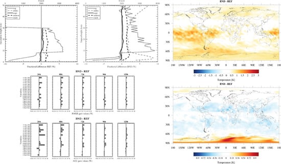
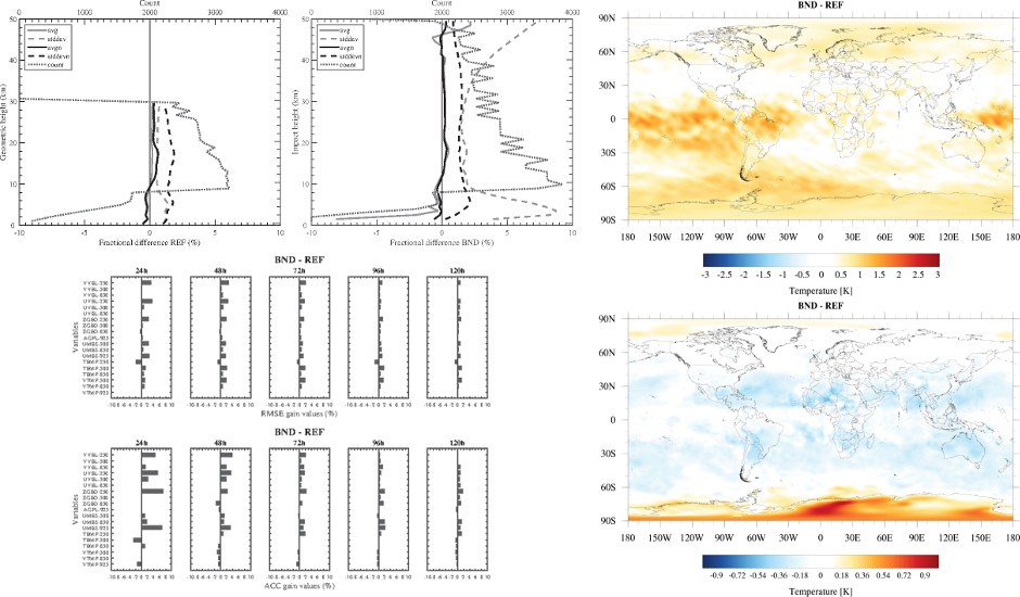
Figure 1 shows the heights that received a larger contribution from GPSRO observations, as in Cucurull et al. [20] but for the global domain. Statistics of the fractional differences between the observed and modeled refractivity are presented in Figure 1a, and between bending angle observations and those simulated from the forecast model in Figure 1b, respectively. The light gray solid curve represents the mean values and the standard deviation is provided by the light gray dashed curve. The count of assimilated observations is shown through the dark gray dotted curve. Simultaneously, Figure 1 presents the results of normalizing the mean (aven, black solid curve) and standard deviation (stddevn, black dashed curve) of the fractional difference values by the mean observation error. Fractional differences were normalized by the mean refractivity error in REF (Figure 1a) and by the mean bending angle error (Figure 1b) in BND. Fractional differences were quantified by layers of 0.5 km in both experiments. The number of assimilated GPSRO observations in each layer is greater in BND than in the REF experiment, mostly between 8 and 15 km where, on average, the high troposphere and low stratosphere are located, respectively. At around 10 km, the number of assimilated GPSRO data in BND increased to approximately 1000 observations more than in REF. The assimilation of less processed data allows more data to be accepted during quality control procedures. Between 30 and 50 km, the extension of the vertical model domain adjusted by the bending angle observations is observed. The curve of the mean remains very close to zero in both experiments indicating that the analyses were highly influenced by the observations. However, a positive increase in the mean and standard deviation (light gray curves) is observed between 45 and 50 km in BND. Few observational systems are able to sample the atmosphere at those heights, thus, the BAM model as probably many others, may have a poor representation of atmospheric systems at this level. In the lower troposphere, at around 2.5 km, an increase in the standard deviation is also observed although with negative mean values. This increase may be related to the high content and horizontal gradients of water vapor, which render the retrieval of GPSRO observations difficult. The vertical distribution of the water vapor can cause simultaneous multiple paths between the transmitter and the receiver, with GPS signals arriving in different ways and data retrieval becoming more difficult [36]. Super-refraction conditions can also lead to a greater bend and delay of the GPS signals; they are sometimes never received at LEO satellites. Refractivity observations suffer more from these situations during data retrieval [39], but bending angles can be affected by super-refraction when calculating the modeled bending angles in the data assimilation process. On the other hand, the bending angle operator in the NBAM assumes spherical symmetry, neglecting horizontal gradients [20], which could limit the results at 2.5 km and below. After normalizing, it is observed that the mean values are closer to zero in BND than in REF. The normalized standard deviation no longer shows an exponential behavior in BND with values of approximately 1.5% over the entire vertical domain, similar to the results in REF. The influence of horizontal gradients remains, to a certain extent, in the troposphere represented by a small increase in the deviation at around 5 km in both experiments. Despite the stratosphere not being directly involved in the development of daily weather systems, stratospheric conditions impose limitations or restrictions on weather and climate variability. An adequate representation of the stratosphere in the forecasting model can increase its predictability, as also achieved when using the sea surface temperature or sea ice cover data [40]. The assimilation of bending angles data is shown to be suitable to improve the predictability of the high-level systems.
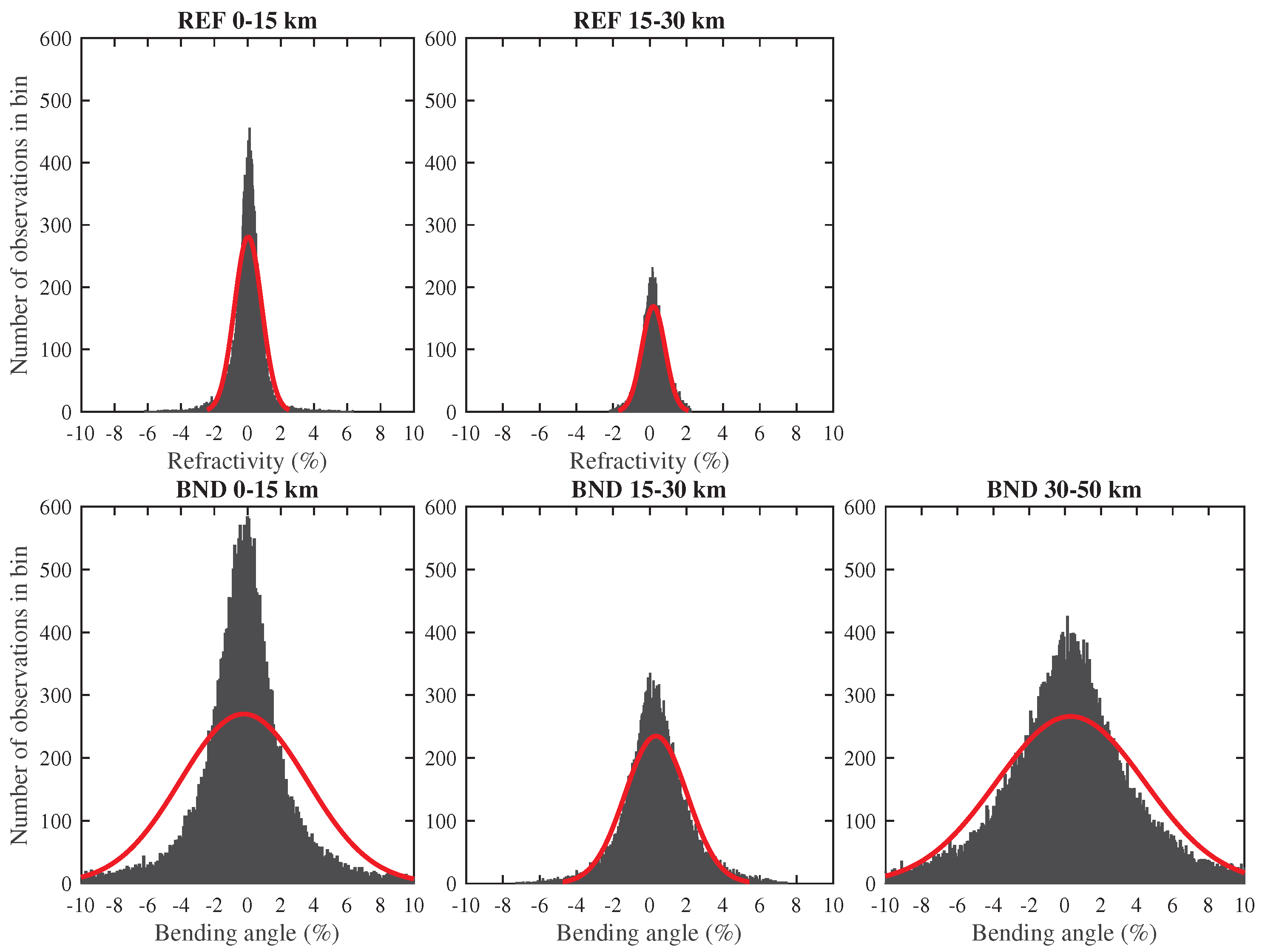
Figure 2 shows frequency histograms of the incremental differences in REF and BND stratified in the vertical domain, for 10 August 2014 at 1200 UTC. This result follows what was proposed in Cucurull et al. [20], but for different ranges of height and showing the normal distribution fit curve. Refractivity profiles were analyzed for heights between 0 and 15 km and 15 and 30 km, including the second value of each interval. As the assimilation of bending angles is extended up to 50 km, results between 30 and 50 km were also analyzed. Both types of observations appear positively deviated from the modeled observations, although refractivity profiles show a less deviated probability density function. The bars in BND are heavier than in REF for all the analyzed heights, indicating a larger amount of differences for each class in the former. Between 0 and 15 km, almost 600 observations are concentrated per bin in BND, whereas 450 are concentrated in REF. At heights between 15 and 30 km, this amount decreases to 330 observations per bin concentrated close to zero in BND and a reduction is also observed in REF to around 220 observations per bin. Between 30 and 50 km, the number of bending angle observations is higher than that in the layers below, up to more than 400 observations per bin around zero. However, at this height, a great number of differences are located in the tail of the histogram, agreeing with the highest values of standard deviation observed in Figure 1b. The standard deviation in the lower atmosphere is also observed in the first heights range in BND through a wider Gaussian curve. The behavior in each interval shows a Gaussian shape with mean difference values located closest to zero, which in turn means that the first-guess is closer to the observations. These results are slightly different from Cucurull et al. [20], where the observations in the last interval showed a clearly non-Gaussian shape curve.
3.3. Cost Function Minimization
Figure 3 presents the mean and standard deviation of the cost functions and gradient norms in each experiment (CNT, REF e BND). The results of all the analyses are shown, generated at 1200 UTC since a greater number of data were available; therefore, a higher efficiency of the process was required. An increase in the values of J is observed from CNT to REF and BND which is directly related to the total of assimilated observations in each case. The highest values of J are reached in BND, with the standard deviation slightly higher than those obtained in the REF and CNT experiments. However, the standard deviation of the gradient norm indicates that similar values are obtained in all the experiments performed. It is noticeable that even with a significant increase in the number of observations in BND (almost twice that in REF), the system converged to the minimum value in the first 50 iterations as in CNT and REF. The obtained results are consistent with our objective since the statistics for all the experiments are quite similar. As the focus in this study is to assess the impact of assimilating less processed GPSRO data in our NWP system, it was configured in a simple form to obtain explicit results, as we can observe in Figure 3. A further study to optimize the minimization process may be conducted in which the execution of more inner and outer loops is assessed.
The fraction of reduction of the initial cost function provided by a group of type x observations during the minimization process was computed as in Cucurull et al. [20]. This analysis is very useful to determine which GPSRO observation type is more costly in the minimization of J. The calculation was carried out using the following formula:
where and are the initial (from the first guess) and final (from the analysis ) total observation cost functions, respectively, and and are the cost function components of the group of type x observations, which are as follows: surface pressure (); temperature (T); wind (W); humidity; GPS (refractivity or bending angle data); and Radiance.
Figure 4 shows the results, in percentage form, for 10 August 2014 at 1200 UTC (Figure 4a) and normalized by the total of assimilated observations of each group (Figure 4b). The largest contribution reducing is accomplished by radiance observations with 64% in BND and 63% in REF. Refractivity profiles indicated 17% reduction and bending angles indicated 17.5% reduction, whereas wind observations contributed to 16% of reduction in BND and 16.5% in REF. Surface pressure, temperature and humidity observations contributed up to 7%. Globally, the high percentage value is found in the radiances because the higher number of assimilated data is from this observation system. However, the greatest contribution is given by the GPS when normalizing by the total of each observation, as shown in Figure 4b where the values are relative. A contribution of was obtained by each refractivity data and by each bending angle observation, while each radiance observation contributes . For temperature, humidity and radiance observations, the greatest reduction was found when assimilating bending angles. However, a somewhat larger contribution remains when assimilating refractivity profiles for wind and pressure surface observations, as well as for GPS themselves where the highest reduction value was achieved in REF. These results are due to the smaller amount of assimilated refractivity data compared to the amount of bending angles being assimilated in BND. Observation operators to assimilate less processed data are more complex than for direct observations. For bending angles, the operator requires the projection of the modeled refractivity into bending angle values and its location [20].
3.4. Analyses Differences
Figure 5 shows the global mean analysis temperature difference between BND and REF at 10 hPa and 850 hPa, respectively. It is observed that at 850 hPa, temperature analyses are slightly cooler in BND than in REF over the tropical latitudes and warmer in the Antarctic region. However, the mean differences are very small varying from −1 to 1 K. At 10 hPa, the differences increase to values between −3 and 3 K, with positive differences over the central Pacific Ocean and the west of the Atlantic Ocean including the tropical region of SA. High latitudes in the SH also show a temperature analysis slightly warmer in BND than in REF. At both levels, it is observed that over the southern high latitudes, on average, temperature analysis is warmer when assimilating bending angle observations. It could indicate that the model is probably routinely cooling the South Pole region and warming tropical latitudes. Figueroa et al. [21] (Figure 1) shows the surface latent heat fluxes averaged for December, January and February in the BAM and Era-Interim reanalysis, where BAM reproduced cooler surface latent heat fluxes in the southern high latitudes with slightly high values over tropical regions for that period. Results in this study suggest that, although the BAM model still needs to be improved, by assimilating bending angles into the NWP system of the CPTEC, it is possible to generate a more realistic initial condition.
3.5. Balance in the First Guess
The initial condition after the data assimilation process should be balanced so as not to degrade weather forecasts. According to Lynch and Huang [41], the unbalance generated from the assimilation process can be measured by computing the mean absolute surface pressure tendency. Wang et al. [42] also used the mean absolute tendency calculation as a measure of high-frequency noise in the forecasts generated using different types of initialization. In this study, we use the mean absolute surface pressure tendency to analyze the surface pressure forecasts that are used as the first guess in the assimilation cycle. Because a FGAT approach was used, the first 9-h forecasts were analyzed. Following Lynch and Huang [41], the mean absolute tendency (N) was calculated as:
where M and N are the points of the entire global domain, is the surface pressure and t is the forecast time. As an indication of balance, the stable oscillation of tendency values around a determined value was considered. Figure 6 shows the mean absolute tendencies in each experiment. Please note that N in BND, REF, and CNT has an initial value of 0.42, 0.39 and 0.3 hPa/h, respectively. Afterwards, the values fall in the second hour of forecasts in all the experiments and then oscillate around approximately 0.25 hPa, which indicates that the 3-, 6- and 9-h forecasts, used as the first guess, are balanced. Although BND shows the larger initial value, which is due to the largest amount of assimilated data in this experiment, the tendency values also fluctuate between 0.25 and 0.27 hPa/h after two forecast hours. The results suggest that the model is not creating or losing mass during the forecast step in the analysis cycle, which contributes to the balanced analysis being obtained.
3.6. Forecasts Skill
The anomaly correlation coefficient (ACC) and RMSE were calculated to evaluate the 120-h forecast. For a better interpretation of the RMSE and ACC results, a Gain Coefficient (GC) was calculated following Sapucci et al. [22]. The GC is very useful to show how important the results were in the forecasts when adding bending angle or refractivity data to the CNT experiment, respectively. This gain is relative to the experiment taken as a control and was calculated using the formulas below:
where v corresponds to any of the variables evaluated at each integration time t, while E indicates the results of the i experiments in which some GPSRO data set was incremented (REF and BND) and C represents the results of the CNT experiment. represents the RMSE value in the case of predictions of a perfect theoretical model, which would imply that it is equal to 0. For the ACC gain, the perfect value corresponds to 1, representing a 100% of correlation between the anomalies of the predicted fields and the analysis in each experiment with respect to the climatology. For both measures, a positive gain value indicates that the experiment adding some GPSRO-type observations benefited the weather forecasts, that is, RMSE values were reduced and ACC values increased. Otherwise, negative values indicate that the addition of this data degrades the forecasts. To highlight where the gains were concentrated, the difference in the RMSE and ACC gain values between BND and REF experiments was calculated for each forecast time, variable and analyzed level.
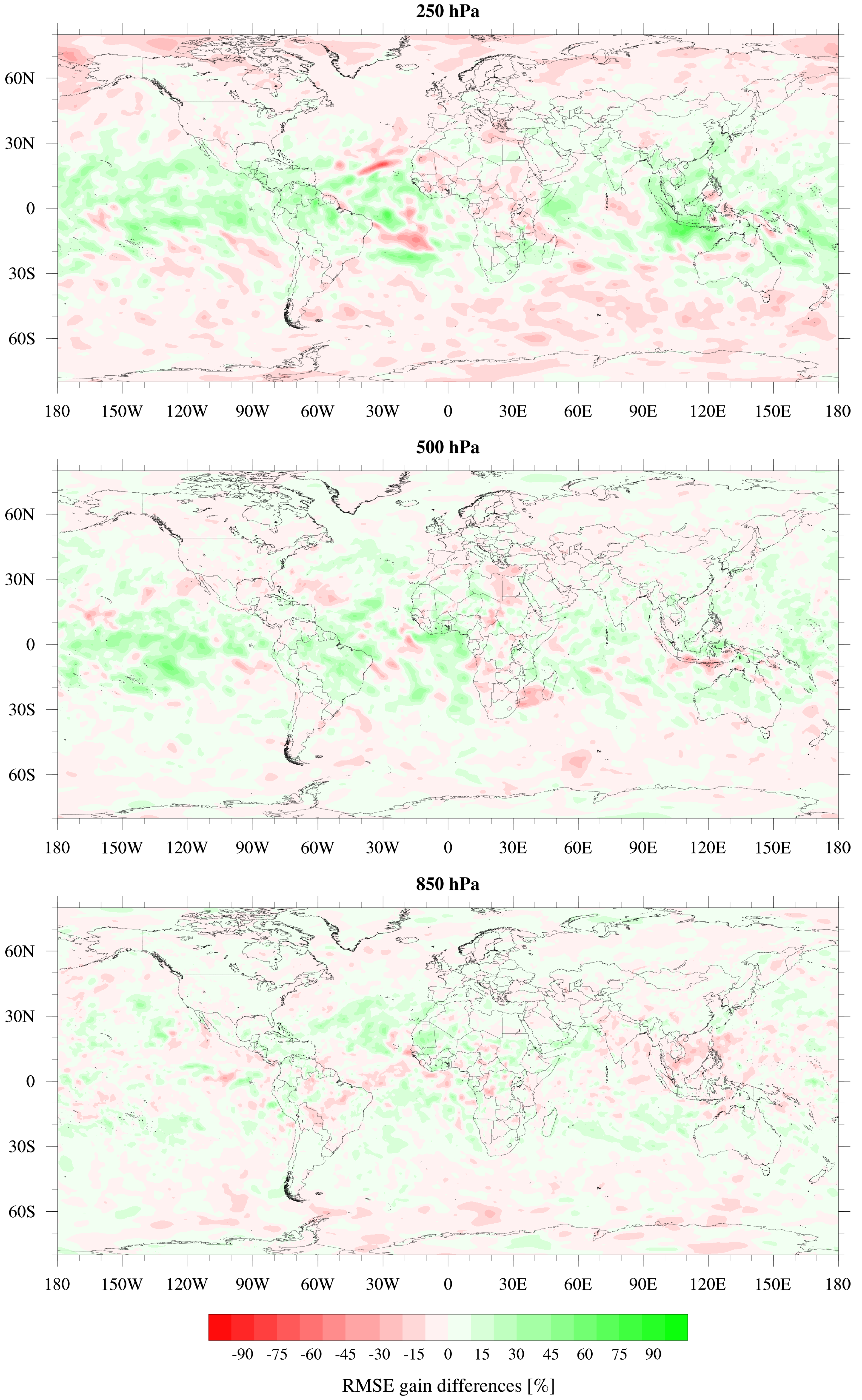
Figure 7 presents results for the mean difference in RMSE gain values for the 12-h temperature forecast at 250, 500, and 850 hPa. Please note that when assimilating bending angles, a noticeable gain in the RMSE values is concentrated in the tropical latitudes between 20S and 20N in the vertical atmospheric column. A reduction in the RMSE is noticeable at 250 hPa where gain values up to 60% are observed. Although, at this level, high values of losses are also reached, throughout the middle and lower atmosphere, the losses are highly reduced showing small values and minor areas at 850 hPa. A gain in the RMSE in BND is also observed over the North and South Poles at 500 and 850 hPa, indicating the positive influence of the bending angle in the temperature analysis. The results from temperature forecasts are representative of the other evaluated variables, which indicate that, probably, the vertical model resolution used (64 vertical sigma levels) may not yet be adequate to assimilate this type of observation that has a high vertical resolution. Furthermore, to fully explore these data, the model should correctly represent atmospheric systems at high levels; however, since there are not many other types of meteorological observations that reliably provide measurements at high atmospheric heights (above 30 km), the model may not appropriately characterize the errors at those heights of the domain. An additional study should be carried out to adjust the background error covariance matrix for the BAM model.
The results of the RMSE and ACC differences are shown in Figure 8. The highest impact in the RMSE gain values is observed when assimilating bending angles during the 5-day forecast for most variables. The RMSE is decreased by 3.5% in the zonal and meridional wind components at 250 hPa, and by 2.5% in the geopotential height also at 250 hPa. These results corroborate the role of GPSRO data assimilation, indirectly impacting mass field forecasts [14]. Virtual and absolute temperature forecasts at 500 and 850 hPa show improvements of about 1 to 2% until the 72-h forecast. For 96- and 120-h forecasts, the enhancements still remain with gains of 0.5 and 1.5%, respectively. The specific humidity forecasts also present gains in the RMSE values when bending angles are assimilated. Gains of 2.5% are observed at 500 and 925 hPa and 1% at 850 hPa for the 24-h forecast. In this variable, a decrease in the RMSE persists for the 120-h lead time in the three evaluated levels with values of 0.5 to 1.8%. The improvements for the specific humidity are remarkable since the BAM has some deficiencies in the precipitation forecast over some regions such as the Amazon and La Plata [21]. The results from the absolute temperature forecast show a degradation in the RMSE gain values at 250 hPa, reaching 2% in the 24-h forecast and diminishing as the forecast time advances. Otherwise, the ACC differences results also show noticeable gain values in the zonal and meridional wind components, geopotential height, and specific humidity by assimilating bending angles. Gain values reach 5.5% and 7% in the wind components at 250 hPa, and specific humidity and geopotential height at 250 hPa, respectively. On average, the forecasts of virtual and absolute temperature show a degradation of 0.5 to 1.5% in BND. Degradation of 2.5% is noted in the absolute temperature at 500 hPa for the 24-h forecast, which becomes neutral in the 48-, 72-, and 96-h forecasts and is again degraded in the 120-h forecast with a loss of 0.5%. Although losses are also found when assimilating bending angles, the results are quite noticeable and suggest the operational use of these data.
Considering the mission of the CPTEC to improve forecasts for the SA region, the Fractional Change (FC) was calculated to highlight the gains in the RMSE over this region. Both the GC and the FC measures are positively oriented, with positive values indicating improvements or positive impacts in the forecasts made. The FC was computed by Equation (5) as recommended in Anthes et al. [43]. The nomenclature used has the same meaning as for the GC formulation.
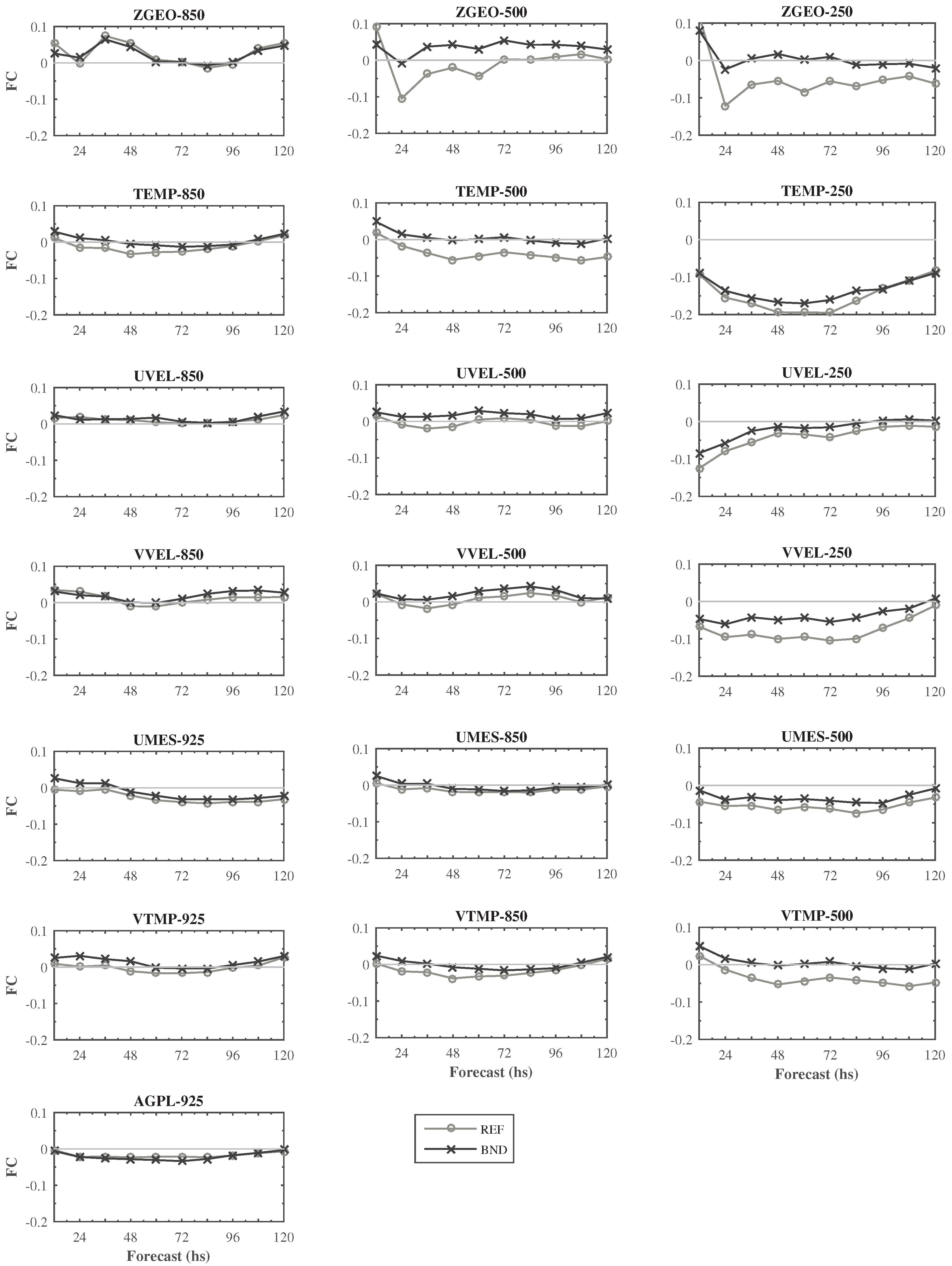
Figure 9 shows the FC values calculated for REF and BND experiments in the SA region, where the zero line is highlighted. The results of FC indicate that in BND the values are more positive than when assimilating the refractivity profiles in most variables. The results obtained for the global domain are also observed over SA, where at 500, 850, and 925 hPa most of the variables show improvements when assimilating bending angles (more FC results reaching the zero value). Temperature forecasts for the 120 h of integration present a low performance at 250 hPa, although small improvements are observed until the 96-h forecast. As mentioned before, the results obtained in this work suggest the need for a study in which the skill of the BAM to represent the atmospheric systems at high levels is investigated and documented; the background error covariance matrix of the BAM should also be appropriately adjusted. Moreover, an increase in the vertical resolution of the model would allow us to further explore the data usage and the precision of the modeled observations from the background.
4. Conclusions
This study presents the first results of the impact of assimilating less processed GPSRO data into the NWP system at the CPTEC, specifically assimilating bending angles over observations of refractivity profiles. Three numerical experiments were conducted—BND, REF and CTN—for August 2014, in which the GPSRO observation used was modified, that is, bending angles compared with refractivity profiles and not using any GPSRO data, respectively. The GSI system was used, coupled to the BAM model. With the assimilation of bending angle data, a greater extension of the vertical domain of the model was impacted, exploring 73.4% of the potential of the RO technique, while with the assimilation of refractivity profiles, less than half of this potential was explored. Despite the exponential behavior of the standard deviation of the fractional differences in BND, it was observed that standard deviation values are similar for the two observation types when normalizing by the mean of the error value in each layer. Although the number of observations of GPSRO is almost doubled using bending angles, the analyses do not require extra computational cost. A further study should be developed to optimize the minimization process in the data assimilation system at the CPTEC.
Regarding the impact on the forecasts, a high impact was clearly observed with the assimilation of bending angles, throughout the model integration time evaluated. The greatest impact of assimilating those data over the refractivity profiles was the RMSE global reduction in almost all the evaluated variables throughout the 5-day forecast. RMSE gain values achieved 3.5% and 2.5% in the zonal and meridional wind components and geopotencial height at 250 hPa, respectively.
The results of the fractional change over South America indicate that the most impacted atmospheric levels were 500 and 850 hPa; however, in BND, at 250 hPa, more positive results were obtained than in REF. The slightly lower performance at the 250 hPa level may be related to the need for a higher vertical resolution of the model and a better representation of the atmosphere at high levels, which should be explored in future research. On the other hand, since there are not many other types of observation systems that reliably provide measurements at higher heights, it is necessary to carry out studies that explore the representation of meteorological systems at those heights and adjust the background error covariance matrix currently in use.
In summary, this study established that the highest gain—after assimilating bending angles into the global data assimilation system of the CPTEC—was the significant increase of the assimilated data throughout the vertical atmospheric column, and especially at the higher levels of the atmosphere. The results reported here are meaningful for the modeling activities at the CPTEC and give clear indications about the improvements in the results due to the best use of GPSRO data, which can guide daily operational assimilation.
Author Contributions
L.F.S. and L.C. had an important role in the design of the study, results discussion and review of the manuscript. C.F.B. and B.B.S. provided scientific and technical support for the coupling of the GSI/BAM system, interpretation of the results and writing of the manuscript. I.H.B. performed the experiments, analyzed the data, generated the figures and wrote the document.
Funding
The first author acknowledges the financial support of the CNPq (acronym in Portuguese for National Council for Scientific and Technological Development) and CAPES (acronym in Portuguese for Coordination for the Improvement of Higher Education Personnel) during her Master and ongoing PhD studies. The APC was funded by the Graduate Program in Meteorology of INPE.
Acknowledgments
The authors thank the CPTEC for providing access to the computational resources used for the development of this research. The Group on Data Assimilation Development and the BAM model developers are also acknowledged for its technical support. We also thank the three anonymous reviewers and the Academic Editor whose comments and suggestions contributed significantly to the improvement of this article.
Conflicts of Interest
The authors declare no conflict of interest.
References
- Bauer, P.; Thorpe, A.; Brunet, G. The quiet revolution of numerical weather prediction. Nature 2015, 525, 47–55. [Google Scholar] [CrossRef] [PubMed]
- Palmer, T.; Hagedorn, R. Predictability of Weather and Climate; Cambridge University Press: Cambridge, UK, 2006; p. 702. [Google Scholar]
- Kalnay, E. Atmospheric Modeling, Data Assimilation, and Predictability; Cambridge University Press: Cambridge, UK, 2003; Volume 54, p. 341. [Google Scholar]
- Kursinski, E.R.; Hajj, G.A.; Bertiger, W.I.; Leroy, S.S.; Meehan, T.K.; Romans, L.J.; Schofield, J.T.; McCleese, D.J.; Melbourne, W.G.; Thornton, C.L.; et al. Initial results of radio occultation observations of Earth’s atmosphere using the Global Positioning System. Science 1996, 271, 1107–1110. [Google Scholar] [CrossRef]
- Eyre, J. Assimilation of Radio Occultation measurements into a numerical weather prediction system. In ECMWF Technical Memoranda; ECMWF: Reading, UK, 1994; p. 22. [Google Scholar]
- Cardinali, C.; Healy, S. Impact of GPS radio occultation measurements in the ECMWF system using adjoint-based diagnostics. Q. J. R. Meteorol. Soc. 2014, 140, 2315–2320. [Google Scholar] [CrossRef]
- Fussen, D.; Tétard, C.; Dekemper, E.; Pieroux, D.; Mateshvili, N.; Vanhellemont, F.; Franssens, G.; Demoulin, P. Retrieval of vertical profiles of atmospheric refraction angles by inversion of optical dilution measurements. Atmos. Meas. Tech. 2015, 8, 3135–3145. [Google Scholar] [CrossRef] [Green Version]
- Kursinski, E.; Hajj, G.; Schofield, J.T.; Linfield, R.P.; Hardy, K.R. Observing Earth’s atmosphere with radio occultation measurements using the Global Positioning System. J. Geophys. Res. 1997, 102, 23429–23465. [Google Scholar] [CrossRef]
- Cardinali, C.; Healy, S. GPS-RO at ECMWF. In Proceedings of the ECMWF Seminar on Data Assimilation for Atmosphere and Ocean, Reading, UK, 6–9 September 2011; pp. 323–336. [Google Scholar]
- Cucurull, L.; Anthes, R.A. Impact of Infrared, Microwave, and Radio Occultation Satellite Observations on Operational Numerical Weather Prediction. Mon. Weather Rev. 2014, 142, 4164–4186. [Google Scholar] [CrossRef]
- Cucurull, L.; Anthes, R.A. Impact of Loss of U.S. Microwave and Radio Occultation Observations in Operational Numerical Weather Prediction in Support of the U.S. Data Gap Mitigation Activities. Weather Forecast. 2015, 30, 255–269. [Google Scholar] [CrossRef]
- Cucurull, L.; Derber, J.C. Operational Implementation of COSMIC Observations into NCEP’s Global Data Assimilation System. Weather Forecast. 2008, 23, 702–711. [Google Scholar] [CrossRef]
- Cucurull, L.; Derber, J.C.; Treadon, R.; Purser, R.J. Assimilation of Global Positioning System Radio Occultation Observations into NCEP’s Global Data Assimilation System. Mon. Weather Rev. 2007, 135, 3174–3193. [Google Scholar] [CrossRef]
- Rennie, M.P. The impact of GPS radio occultation assimilation at the Met Office. Q. J. R. Meteorol. Soc. 2010, 136, 116–131. [Google Scholar] [CrossRef]
- Healy, S.B.; Thepaut, J.N. Assimilation experiments with CHAMP GPS radio occultation measurements. Q. J. R. Meteorol. Soc. 2006, 132, 605–623. [Google Scholar] [CrossRef] [Green Version]
- Bonavita, M. On some aspects of the impact of GPSRO observations in global numerical weather prediction. Q. J. R. Meteorol. Soc. 2014, 140, 2546–2562. [Google Scholar] [CrossRef]
- Cucurull, L.; Kuo, Y.H.; Barker, D.; Rizvi, S.R.H. Assessing the Impact of Simulated COSMIC GPS Radio Occultation Data on Weather Analysis over the Antarctic: A Case Study. Mon. Weather Rev. 2006, 134, 3283–3296. [Google Scholar] [CrossRef]
- Cucurull, L.; Derber, J.C.; Treadon, R.; Purser, R.J. Preliminary Impact Studies Using Global Positioning System Radio Occultation Profiles at NCEP. Mon. Weather Rev. 2008, 136, 1865–1877. [Google Scholar] [CrossRef]
- Cucurull, L. Improvement in the Use of an Operational Constellation of GPS Radio Occultation Receivers in Weather Forecasting. Weather Forecast. 2010, 25, 749–767. [Google Scholar] [CrossRef]
- Cucurull, L.; Derber, J.C.; Purser, R.J. A bending angle forward operator for global positioning system radio occultation measurements. J. Geophys. Res. Atmos. 2013, 118, 14–28. [Google Scholar] [CrossRef] [Green Version]
- Figueroa, S.N.; Bonatti, J.P.; Kubota, P.Y.; Grell, G.A.; Morrison, H.; Barros, S.R.M.; Fernandez, J.P.R.; Ramirez, E.; Siqueira, L.; Luzia, G.; et al. The Brazilian Global Atmospheric Model (BAM): Performance for Tropical Rainfall Forecasting and Sensitivity to Convective Scheme and Horizontal Resolution. Weather Forecast. 2016, 31, 1547–1572. [Google Scholar] [CrossRef]
- Sapucci, L.F.; Diniz, F.L.R.; Bastarz, C.F.; Avanço, L.A. Inclusion of Global Navigation Satellite System radio occultation data into Center for Weather Forecast and Climate Studies Local Ensemble Transform Kalman Filter (LETKF) using the Radio Occultation Processing Package as an observation operator. Meteorol. Appl. 2016, 23, 328–338. [Google Scholar] [CrossRef] [Green Version]
- Azevedo, H.B.D.; Gonçalves, L.G.G.D.; Bastarz, C.F.; Silveira, B.B. Observing System Experiments in a 3DVAR Data Assimilation System at CPTEC/INPE. Weather Forecast. 2017, 32, 873–880. [Google Scholar] [CrossRef]
- Cavalcanti, I.F.; Marengo, J.A.; Satyamurty, P.; Nobre, C.A.; Trosnikov, I.; Bonatti, J.P.; Manzi, A.O.; Tarasova, T.; Pezzi, L.P.; D’Almeida, C.; et al. Global climatological features in a simulation using the CPTEC-COLA AGCM. J. Clim. 2002, 15, 2965–2988. [Google Scholar] [CrossRef]
- Davies, R.; Randall, D.A.; Corsetti, T.G. A fast radiation parameterization for atmospheric circulation models. J. Geophys. Res. 1987, 92, 1009–1016. [Google Scholar] [Green Version]
- Chou, M.D.; Suarez, M.J. A Solar Radiation Parameterization Atmospheric Studies. In Technical Report Series on Global Modeling and Data Assimilation; NASA: Washington, DC, USA, 1999. [Google Scholar]
- Grell, G.A.; Dévényi, D. A generalized approach to parameterizing convection combining ensemble and data assimilation techniques. Geophys. Res. Lett. 2002, 29, 38-1–38-4. [Google Scholar] [CrossRef]
- Tiedtke, M. The sensitivity of the time-mean large-scale flow to cumulus convection in the ECMWF model. In Proceedings of the ECMWF Workshop on Convection in Large-Scale Models, Shinfield Park, Reading, 28 November–1 December 1983; European Centre for Medium-Range Weather Forecasts: Reading, UK, 1983; pp. 297–316. [Google Scholar]
- Xue, Y.; Sellers, P.; Kinter, J.; Shukla, J. A Simplified Biosphere Model for Global Climate Studies. J. Clim. 1991, 4, 345–364. [Google Scholar] [CrossRef] [Green Version]
- Holtslag, A.A.M.; Boville, B.A. Local versus nonlocal boundary-layer diffusion in a global climate model. J. Clim. 1993, 6, 1825–1842. [Google Scholar] [CrossRef]
- Mellor, G.; Yamada, T. Development of a turbulence closure for geophysical fluid problems. Rev. Geophys. Space Phys. 1982, 20, 851–875. [Google Scholar] [CrossRef]
- Developmental Testbed Center. Gridpoint Statistical Interpolation (GSI) User’s Guide for Version 3.3. In Community Gridpoint Statistical Interpolation System; Developmental Testbed Center: Boulder, CO, USA, 2014; p. 108. [Google Scholar]
- Campos, T.B.; Sapucci, L.F.; Lima, W.; Ferreira, D.S. Sensitivity of Numerical Weather Prediction to the Choice of Variable for Atmospheric Moisture Analysis into the Brazilian Global Model Data Assimilation System. Atmosphere 2018, 9, 123. [Google Scholar] [CrossRef]
- Bevis, M.; Businger, S.; Chiswell, S.; Herring, T.A.; Anthes, R.A.; Rocken, C.; Ware, R.H. GPS Meteorology: Mapping Zenith Wet Delays onto Precipitable Water. J. Appl. Meteorol. 1994, 33, 379–386. [Google Scholar] [CrossRef] [Green Version]
- Rüeger, J.M. Refractive Index Formulae for Radio Waves. In Proceedings of the JS28 Integration of Techniques and Corrections to Achieve Accurate Engineering, FIG Proceedings XXII International Congress, Washington, DC, USA, 19–26 April 2002; pp. 19–23. [Google Scholar]
- Jin, S.; Cardellach, E.; Xie, F. GNSS Remote Sensing; Springer: Berlin, Germany, 2014; Volume 19, pp. 215–239. [Google Scholar]
- Desroziers, G.; Berre, L.; Chapnik, B.; Poli, P. Diagnosis of observation, background and analysis-error statistics in observation space. Q. J. R. Meteorol. Soc. 2005, 131, 3385–3396. [Google Scholar] [CrossRef] [Green Version]
- Lee, M.S.; Barker, D.; Huang, W.; Kuo, Y.H. First Guess at Appropriate Time (FGAT) with WRF 3DVAR. J. Korean Meteorol. Soc. 2005, 41, 495–505. [Google Scholar]
- Syndergaard, S. On the ionosphere calibration in GPS radio occultation measurements. Radio Sci. 2000, 35, 865–883. [Google Scholar] [CrossRef] [Green Version]
- Karpechko, A.; Tummon, F.; Secretariat WMO. Climate Predictability in the Stratosphere. Bull. World Meteorol. Organ. 2016, 65, 54–57. [Google Scholar]
- Lynch, P.; Huang, X.Y. Initialization of the HIRLAM Model Using a Digital Filter. Mon. Weather Rev. 1992, 120, 1019–1034. [Google Scholar] [CrossRef] [Green Version]
- Wang, H.G.; Wu, Z.S.; Kang, S.F.; Zhao, Z.W. Monitoring the marine atmospheric refractivity profiles by ground-based GPS occultation. IEEE Geosci. Remote Sens. Lett. 2013, 10, 962–965. [Google Scholar] [CrossRef]
- Anthes, R.A.; Ector, D.; Hunt, D.C.; Kuo, Y.H.; Rocken, C.; Schreiner, W.S.; Sokolovskiy, S.V.; Syndergaard, S.; Wee, T.K.; Zeng, Z.; et al. The COSMIC/FORMOSAT-3 Mission: Early Results. Bull. Am. Meteorol. Soc. 2008, 89, 313–333. [Google Scholar] [CrossRef]
Figure 1.
Statistics of the fractional differences ((O-B)/B) (avg and stddev) and normalized by the error observation (avgn and stddevn), between (a) the observations and modeled refractivity profiles as a function of the geometric height and (b) the observations of bending angles and those simulated from the model as a function of the impact height. Count refers to the total refractivity (a) and bending angle (b) observations assimilated in each experiment.

Figure 2.
Frequency histograms of the differences between the observations and background by height intervals, in the REF (upper panels) and BND (lower panels) experiments, referring to the analysis generated on 10 August 2014 at 1200 UTC. Red curves represent the normal distribution fit curve in each height range.

Figure 3.
Statistics of the cost functions and gradient norms for the CNT, REF, BND experiments at 1200 UTC.
Figure 3.
Statistics of the cost functions and gradient norms for the CNT, REF, BND experiments at 1200 UTC.
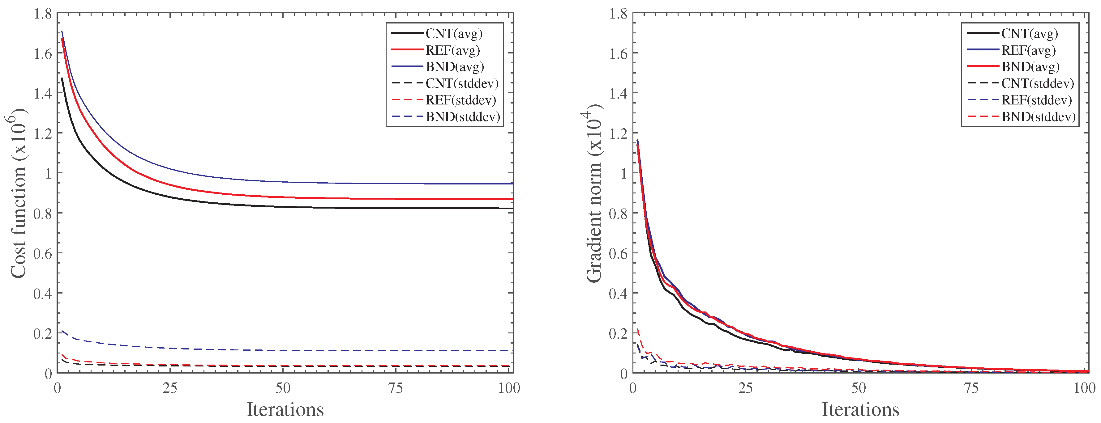
Figure 4.
Contribution of (a) each type of observation (in %) and (b) each type of observation normalized by the number of observations used in each case, in the reduction of the total cost function in the analysis generated for 10 August 2014 at 1200 UTC.
Figure 4.
Contribution of (a) each type of observation (in %) and (b) each type of observation normalized by the number of observations used in each case, in the reduction of the total cost function in the analysis generated for 10 August 2014 at 1200 UTC.

Figure 5.
Mean difference between BND and REF temperature analysis at (a) 10 hPa and (b) 850 hPa, for August 2014.
Figure 5.
Mean difference between BND and REF temperature analysis at (a) 10 hPa and (b) 850 hPa, for August 2014.

Figure 6.
Mean absolute surface pressure tendency in each experiment over the global region for the period under study.
Figure 6.
Mean absolute surface pressure tendency in each experiment over the global region for the period under study.
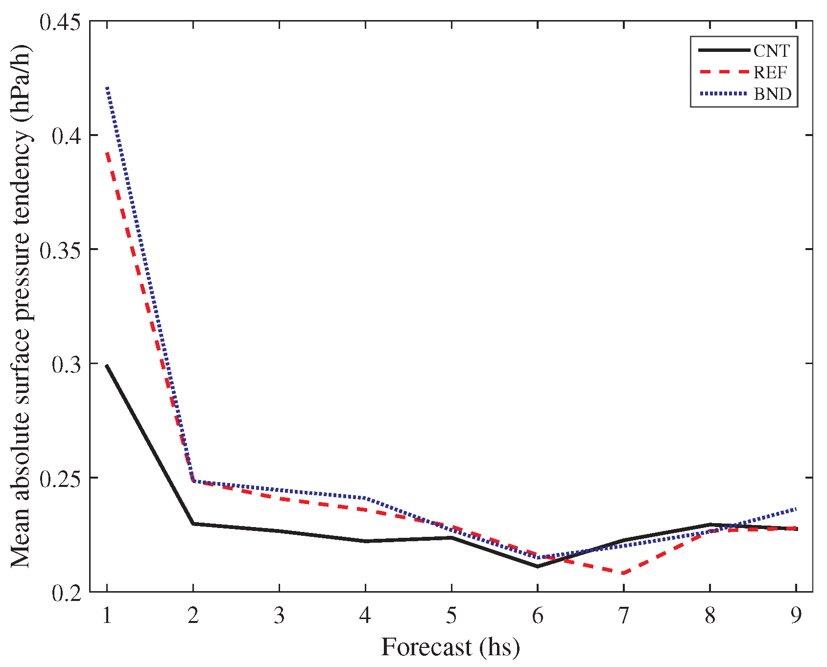
Figure 7.
Mean difference in the RMSE gain between BND and REF for the 12-h temperature forecast at 250, 500 and 850 hPa (from top to bottom), for August 2014. Green values indicate a gain in the RMSE values, while red values indicate a loss.
Figure 7.
Mean difference in the RMSE gain between BND and REF for the 12-h temperature forecast at 250, 500 and 850 hPa (from top to bottom), for August 2014. Green values indicate a gain in the RMSE values, while red values indicate a loss.

Figure 8.
Differences in RMSE and ACC gain values for all variables (represented on the ordinate axis) for: 24-, 48-, 72-, 96- and 120-h forecasts (from left to right, respectively) over the global region.
Figure 8.
Differences in RMSE and ACC gain values for all variables (represented on the ordinate axis) for: 24-, 48-, 72-, 96- and 120-h forecasts (from left to right, respectively) over the global region.

Figure 9.
Fractional change of the RMSE values for all variables evaluated and the 120 h of model integration over the South America region.
Figure 9.
Fractional change of the RMSE values for all variables evaluated and the 120 h of model integration over the South America region.


Table 1.
Parameterizations of physical processes in the BAM model used in this study.
| Long-wave radiation | Harshvardhan et al. [25] |
| Short-wave radiation | CliRAD (Chou and Suarez [26]) |
| Deep convection | Grell and Dévényi [27] |
| Shallow convection | Tiedtke [28] |
| Surface scheme | SSIB (Xue et al. [29]) |
| Boundary layer top | Holtslag and Boville [30] |
| Boundary layer bottom | Mellor and Yamada [31] |
Table 2.
Values of the refractivity coefficients available in GSI v3.3.
| Rüeger [35] | Bevis et al. [34] | Unit | |
|---|---|---|---|
| 77.6890 | 77.60 | K mb | |
| 3.75463 | 3.739 | K mb | |
| 71.2952 | 70.4 | K mb |
Table 3.
Configuration of the experiments conducted in this study.
| CNT | REF | BND |
|---|---|---|
| Conventional data | Conventional data | Conventional data |
| Unconventional data | Unconventional data | Unconventional data |
| (Radiances) | (Radiances) | (Radiances) |
| (No GPSRO data) | (GPSRO refractivity profiles) | (GPSRO bending angles) |
Table 4.
Number of available observations and those assimilated in each experiment.
| BND | % | REF | % | |
|---|---|---|---|---|
| Number of available observations | 21,385.736 | 100 | 20,935.518 | 97.9 |
| Assimilated observations | 15,688.745 | 73.4 | 9002.718 | 42.1 |
| 0–30 km | 9736.151 | 45.5 | 9002.718 | 42.1 |
| 30–50 km | 5952.594 | 27.8 | - | - |
| Not Assimilated observations | 5696.991 | 26.6 | 11,932.800 | 55.8 |
© 2019 by the authors. Licensee MDPI, Basel, Switzerland. This article is an open access article distributed under the terms and conditions of the Creative Commons Attribution (CC BY) license (http://creativecommons.org/licenses/by/4.0/).
Share and Cite
MDPI and ACS Style
Banos, I.H.; Sapucci, L.F.; Cucurull, L.; Bastarz, C.F.; Silveira, B.B. Assimilation of GPSRO Bending Angle Profiles into the Brazilian Global Atmospheric Model. Remote Sens. 2019, 11, 256. https://doi.org/10.3390/rs11030256
AMA Style
Banos IH, Sapucci LF, Cucurull L, Bastarz CF, Silveira BB. Assimilation of GPSRO Bending Angle Profiles into the Brazilian Global Atmospheric Model. Remote Sensing. 2019; 11(3):256. https://doi.org/10.3390/rs11030256
Chicago/Turabian StyleBanos, Ivette H., Luiz F. Sapucci, Lidia Cucurull, Carlos F. Bastarz, and Bruna B. Silveira. 2019. "Assimilation of GPSRO Bending Angle Profiles into the Brazilian Global Atmospheric Model" Remote Sensing 11, no. 3: 256. https://doi.org/10.3390/rs11030256
Note that from the first issue of 2016, this journal uses article numbers instead of page numbers. See further details here.