Evaluation of the Effect of Urban Redevelopment on Surface Urban Heat Islands


1
University Jean Moulin Lyon 3, UMR CNRS Environment City Society, 69007 Lyon, France
2
National Aeronautics and Space Administration NASA, Goddard Space Flight Center, Greenbelt, MD 20771, USA
3
University of Edinburgh, Edinburgh, EH8 9YL, Scotland, UK
*
Author to whom correspondence should be addressed.
Remote Sens. 2019, 11(3), 299; https://doi.org/10.3390/rs11030299
Submission received: 31 December 2018
/
Revised: 28 January 2019
/
Accepted: 28 January 2019
/
Published: 1 February 2019
(This article belongs to the Special Issue Urban Heat Island Remote Sensing)
Abstract
:Climate change is a global challenge with multiple consequences. One of its impacts is the increase in heatwave frequency and intensity. The risk is higher for populations living in urban areas, where the highest temperatures are generally identified, due to the urban heat island effect. This phenomenon has recently been taken into account by local elected officials. As a result, developers have decided to use solutions in redevelopment projects to combat high temperatures in urban areas. Consequently, the objective is to study the land-surface temperature evolution of six main urban redevelopments in Lyon, France, from 2000 to 2017. Three of them (the Confluence, Kaplan, and Museum sites) were composed of industrial areas that have undergone major transformations and are now tertiary or residential areas. Two sites have been more lightly transformed, particularly by increasing vegetation to reduce heat stress and urban flooding (Dock and Garibaldi Street). Finally, the Groupama Stadium has been built into agricultural and wooded areas. Changes in vegetation cover (NDVI), water (MNDWI), and moisture (NDMI) content, built areas (NDBI) and bare soil (NDBaI) are also monitored. The results show that the Confluence and Kaplan sites were accompanied by a decrease in surface temperature and an increase in vegetation and moisture, whereas the Groupama Stadium displayed a rise in surface temperature and a decrease in vegetation. On the other hand, the Museum, Dock, and Garibaldi sites did not exhibit clear and uniform trends, although an increase in surface temperature was shown in some statistical tests. The disparity of the results shows the necessity to include a significant amount of vegetation during redevelopment operations in order to reduce heat stress.
1. Introduction
According to the Intergovernmental Panel on Climate Change, the current climate change is likely to increase the intensity and frequency of extreme events [1]. This is particularly the case for heatwaves, the severity of which has increased in Europe in recent decades [2,3]. In addition, rising temperatures due to global climate change is amplified by the effect of urban heat islands [4]. This phenomenon is widely analyzed and is one of the major themes of urban climatology, particularly its impact on human health [5]. An Urban Heat Island (UHI) is characterized by a difference in temperature between an urban area and the surrounding rural environments. Generally, the temperature of urban areas is higher than in rural areas, especially at night. However, exceptions may exist, such as in cities like Las Vegas or Madrid (heat sink [6,7,8]).
Typically, there are three distinct UHI types: canopy UHI, boundary-layer UHI, and surface UHI. The urban canopy is the layer between the ground and building rooftops, and it is strongly influenced by surface, morphological, and anthropic parameters. The boundary layer is just above the canopy layer, and is affected by both the microscale processes taking place underneath it, as well as the mesoscale processes taking place above it [8,9,10,11]. The key parameter in characterizing the boundary-layer UHI is air temperature. These two types of UHI are complemented by the study of surface UHIs (SUHIs), which is based on the measurement of land-surface temperatures (LST) that directly influence air temperature in the canopy layer by energy exchange [9,11,12,13]. This study concentrates on SUHI because of the lack of ground measurements on the study sites.
Heat intensification can be explained primarily by the surface parameters related to the replacement of vegetation cover, wetlands, and water surfaces by artificial surfaces, resulting in low evaporation and evapotranspiration. This effect is combined with the effect caused by buildings made of low albedo materials with high thermal inertia, which absorb and store heat, often leading to a thermal time lag of a few hours depending on the size and type of the buildings and climate. Morphological parameters related to urban roughness and the sky-view factor can also be the reasons for an increase of UHIs. The former can provoke a reduction of the wind speed and the latter can limit the release of heat at night [14]. However, urban density associated with very tall buildings can also have a cooling effect because of their projected shadow, which helps to minimize increases in the intensity of the early night-time UHI [15]. Finally, there are also anthropogenic parameters such as industrial heat emissions, heating, transport, or air conditioning. Therefore, it is common to find higher temperatures in urban areas compared to rural areas, ranging from about 5 to 10 °C during favorable weather conditions, that is, clear skies and no wind [9].
Thermal gradients can be quantified in different ways. For air-temperature measurements, fixed measurements are most often used. However, urban-monitoring networks are generally not dense enough to characterize the processes occurring on such a small scale [16]. Thus, mobile measurements can be used, operating by transect, though they are not continuous in time, contrary to a ground measurement network [17,18]. Surface temperatures are most often measured by remote sensing using satellites. Upwelling thermal radiance is initially measured and is then converted into surface temperature through different algorithms [19]. Sometimes, surface temperature is collected by thermal imagers on board aircrafts or from a high point overlooking the study site. It can be noted that air temperature and the LST are two different parameters that should not be confused: air temperature concerns the canopy layer, whereas LST is a two-dimensional measurement of thermal infrared data obtained by remote sensing. The latter is often a few degrees higher than the former given optimal conditions for surface-temperature measurement [9,10]. In addition, areas with the highest LSTs may not exactly correspond to those with the highest ambient air temperature, and the linear relationship between these two parameters is sometimes not obvious [8,11,20]. Furthermore, more qualitative UHI measurements can be obtained by collecting data in situ, involving asking users about their thermal sensitivity and site practice through questionnaires, interviews, or mental maps, for example [21,22,23]. In addition, the participation of users in the process can mobilize and raise awareness of the phenomenon of thermal discomfort. However, in addition to the subjectivity of the responses, the representability of the data collected may remain partial depending on the number and panel of respondents.
UHI has consequences on the energy consumption necessary for household air conditioning, but also especially has an impact on human health. Indeed, heat can cause thermal stress and lead to risks of sunstroke, dehydration, hyperthermia, and heat stroke. The most sensitive people are the elderly, infants, young children, and sick people [24,25]. In addition to physical fitness, social vulnerability is also an important risk factor with unsuitable housing or isolated communities [26].
The 2003 heatwave caused an excess mortality of 70,000 deaths in Europe [27]. More locally, in France, the heatwaves of 2003, 2006, and 2015 respectively caused 19,490, 1388, and 3275 deaths according to the International Disaster Database EM-DAT (https://www.emdat.be/). During the 2003 heatwave in Paris, excess mortality was 141% higher than the summer average, and 80% higher in Lyon, the second-largest city in France [28,29]. In addition, an increase in surface UHI of around 0.5 °C could be the cause of these doubling mortality rates [30]. Victims were mainly counted in large cities. This phenomenon is concerning given that more than half of the world’s population currently lives in urbanized areas according to the Population Reference Bureau (https://www.prb.org/), and thus a large portion of the population is exposed to it. The problem will only worsen, seeing as, by 2050, 70% of the population is predicted to live in urban areas, with no apparent trend reversal [31].
Solutions must be found through urban-planning policies by implementing sustainable adaptation strategies, such as those recommended by the European Climate Adaptation Platform, in particular by increasing green and shaded areas [15] in order to improve the thermal comfort of the inhabitants [8,14,32]. Solutions should begin with a better understanding of UHIs, and an assessment of the effect of urban development and temperature renewal.
Previous studies have mainly focused on studying differences in ground temperatures as a function of land-use land cover and its evolution at the city level [16,16,20,33,34,35], temporal trends in urban SUHI in urban areas [18,36,37], the refreshing impact of parks on their surroundings [15,38,39], the evolution of SUHI as a function of day and night [9,34,40,41], the impact of vegetation on LST at the urban scale [12,36,37,42], comparison of surface temperatures and air temperature [8,9,10,20,43,44], the impact of surface temperatures on health [30,41] and transversely at surface temperatures at moderate resolutions (MODIS 1 km) [16,20,34,35,36,42,45] but, to our knowledge, there are no similar studies such as ours that analyze the thermal monitoring of site redevelopment at such a detailed spatial and temporal resolution.
Consequently, this study focuses on six urban sites in the Lyon metropolitan area that have been the target of major redevelopments. The objective is to compare the evolution of surface temperatures, as well as humidity or vegetation spectral indices (among others) of these sites, obtained for days of similar climatic conditions, ante- and post-redevelopment. The data are recovered from the measurement campaigns of Landsat satellite sensors, as MODIS data are of too-low resolution for the purposes of this study. First, the connections between these different spectral indices and the surface temperature are explored to identify which indices most influence temperatures. Quantifying the effects of land-use changes on urban microclimates provides urban planners with valuable information on the impact of certain land-cover types, which helps in the decision-making process. Secondly, the study area is presented, as well as the remote-sensing data and statistical methods. Thirdly, the results are shown and analyzed to discuss their implications and how they contribute to the improvement of urban planning in the context of UHI mitigation.
2. Materials and Methods
2.1. Study Area
The Lyon metropolis (45°45′35″ N, 4°50′32″ E) is located in southeastern France, and it is the second-largest French metropolitan area after Paris, with a total population of 2.2 million (Figure 1). It is characterized by a warm temperate climate with Mediterranean influences, with high temperatures in spring and summer (Köppen classification: Cfa or Cfb). The hottest months are from June to September, with a maximum daily temperature ranging from 24.6 to 27.7 °C, and average relative humidity at around 55%. Since 1921 (start of the measurements at the Lyon-Bron weather station, part of Météo-France network), the coldest temperature and the warmest temperature have been rising according to the Mann–Kendall trend test [46] (Kendall’s tau (τ) = 0.558 and τ = 0.285, respectively; probability value (p-value) < 0.0001).
2.2. Site Selection
This study does not aim to be an exhaustive analysis of all redevelopments in Lyon since the 2000s. It is based on a critical selection of the most emblematic and interesting sites from a land-management point of view. In addition, it is necessary to have a time lag of a few years after site redevelopment in order to assess the consequences of the work. An inventory of these redevelopments was carried out and led to a selection of six sites with different morphological characteristics (Figure 1): Confluence, Garibaldi Street, Kaplan Park, the dock, the museum, and Groupama Stadium. These sites, initially highly urbanized, were redeveloped between the end of 2005 and 2012, with an increase in vegetation cover to reduce heat stress and urban flooding except for the Groupama Stadium area. The Groupama Stadium is complementary to the other sites because it was built from 2013 to 2015 within an agricultural areas and is not a renewal project.
Three sites have undergone major renovations: Confluence, Kaplan Park, and the museum. The Confluence site (transformed from 2005 to 2009 at a cost of €1.165 billion) was originally an industrial and wholesale-market site. Currently, it is a largely residential sector, with a shopping center of more than 50,000 m2. A water basin (2 ha) was created and the site was heavily revegetated (Figure 2). The work on Jacob Kaplan Park took place at the same time, turning the former industrial wasteland into a more modern district, with a school complex, a gymnasium, and residential and office buildings (€1.25 million, Figure 2). From 2006 to 2014, the museum (Musée des Confluences) was built into an industrial area except for the southern part, which is covered by grass. The area is now composed of a huge building (190 m long, 90 m wide, and 41 m high), a waterproofed square in front, and a landscaped area behind it, at a final cost of €330 million (Figure 2).
Two sites have been the subject of lighter developments: the docks and Garibaldi. The docks were an open-air car park (1600 spaces), and were then transformed into an urban park (10 ha—350 trees, 6000 m2 of lawn) that connects the two main parks in the northern (Gerland) and southern (Tête d’or) parts of the city (approximately €2 million on the study site—Figure 3). Garibaldi Street was a typical urban highway during the 1960s with hoppers to facilitate traffic. Now, the area is calmer, with less car traffic, thanks to bicycle paths and improved public transport, as well as landscaped wooded areas for sustainable stormwater management. It creates a green continuity from the Tête d’or Park (north of the urban center) to Blandan Park (east of the urban area—€30 million).
The last site is the Groupama Stadium. It is the new stadium of the OL football team (www.ol.fr). This team’s matches were previously held in a dilapidated stadium in the city center. Groupama Stadium (€410 million) was built on agricultural and wooded land in the eastern part of the city to provide a larger-capacity stadium (around 60,000 seats) that meets the latest safety standards (Figure 4).
2.3. Landsat and Meteorological Data
The data were acquired from the TM, ETM+, and OLI/TIRS sensors on board the Landsat 5, 7, and 8 satellites. The study period chosen is between 2000 and 2017 in order to be able to study the six study sites before and after their transformation. Due to overlapping paths 196 (left margin) and 197 (right margin, row 28), a large number of suitable scenes with zero cloud cover, haze, and fog cloud could be obtained within the study period.
The procedure of selecting images and analysis dates was carried out in two stages. First, all available Landsat 5, 7, and 8 images on the study sites since 2000 for the months of June to August were downloaded from the EarthExplorer website and analyzed. Images with no cloud cover on the six sites were selected. In a second step, a selection of one image per year was made. It is impossible to study the same days each year due to the passage of Landsat and changing weather conditions, even in summer. Then, days with similar climatic conditions were selected for each of the study years, reflecting hot weather with little or no wind under anticyclonic conditions (Table 1). The parameters used to select the days were temperature, precipitation, relative humidity, average wind direction and speed, and pressure. The reference station is Lyon-Bron from Météo-France. Cloud cover was provided by Landsat metadata. The meteorological homogeneity of the chosen days was verified using the Pettitt test [47], the Standard Normal Homogeneity Test (SNHT) [48], the Buishand test [49], and the von Neumann [50] test, which showed no significant differences (significance level α = 0.05). In addition, the meteorology of the two previous days for each scene was checked to ensure climate continuity, for example to detect possible rain showers that would have impacted surface temperature, for example (Table 2). No days were selected in 2000 and from 2006 to 2012 due to the inability to find suitable images as a result of either cloud cover or large discrepancies in weather conditions. This time gap is not a major problem for the study because this period corresponds to the transformation phases of the study sites. As a result, the ante- and postdevelopment conditions are still comparable.
2.4. TIR Data Conversion to LST
Landsats 5, 7, and 8 carry different sensors (TM, ETM+, and OLI/TIRS sensors). Visible, near-infrared, short-wavelength infrared, panchromatic, and cirrus bands (when available) have a spatial resolution of 30 m. TM Band 6 is at a resolution of 120 m, ETM+ Band 6 is at a 60 m resolution, and the TIRS bands are at a 100 m resolution, but at 30 m resolution in the delivered data product after resampling with cubic convolution by the United States Geological Survey (USGS) [51].
There are three main ways to estimate LST from Landsat 8 data: the radiative-transfer equation, the split-window (SW) algorithm, and the single-channel (SC) method. The SW algorithm uses two thermal bands located around 10 and 12 µm, but it is not suitable for TM and ETM+ sensors, which have only one available thermal band. Furthermore, the USGS advises to only use TIRS Band 10, which has fewer expected errors caused by stray light anomalies compared to Band 11 (before 24 April 2017) [52,53].
Although NASA has corrected all L8 TIR data, they recommend not using SWA for atmospheric correction [54]. Nevertheless, the stray light-corrected L8 TIRS data are used in this study.
In this study, surface-temperature estimation is performed using the SC algorithm since this method has been applied to Landsat 5 TM, Landsat 7 ETM+, MODIS, ASTER, and ENVISAT AATSR sensors’ TIR bands for research in urban thermal conditions with appropriate accuracy [12,19,42,55]. This method was developed by research mainly done by Jimenez-Munoz et al., Sobrino et al., and Qin et al. [56,57,58,59].
Atmosphere affects thermal radiation received by the satellites. Consequently, a precise temperature cannot be directly measured by TM, ETM+, and TIRS sensors. The spectral response of objects in thermal infrared regions (10.40–2.50 µm for Band 6 for TM and ETM+ sensors, and 10.60–11.19 µm and 11.50–12.51 µm for Bands 10 and 11, respectively, for the TIRS sensor) is stored as digital numbers (DNs) or Quantized and calibrated standard product pixel values (Qcal). Their values range from 0 to 255, and are delivered in an 8-bit (for TM and ETM+) or 16-bit unsigned integer format [43]. Consequently, the preliminary step for calculating surface temperature is to obtain brightness temperature, as stated by USGS [60].
- Step 1: conversion to top of atmosphere (TOA) Radiance, Equation (1):
Lλ = ML·Qcal + AL
- Lλ = TOA spectral radiance for wavelength λ (Watts/(m2 * srad * μm))
- ML = Band-specific multiplicative radiance rescaling factor from the metadata (in the MTL file)
- Qcal = Quantized and calibrated standard product pixel values (DN)
- AL = Band-specific additive radiance rescaling factor from the metadata (in the MTL file)
Markham and Barker also proposed another way to calculate spectral radiance [43,61], Equation (2):
Lλ = Lmin(λ) + (Lmax(λ) − Lmin(λ)) Qdn/Qmax
- Qdn = grey level of each pixel
- Qmax = maximum numerical value of the pixel
- Lmax(λ) = minimum spectral radiance for Qdn = 0
- Lmin(λ) = maximum spectral radiance for Qdn = 255
- Step 2: conversion to at-satellite brightness temperature
The transformation of at-sensor spectral radiance to at-sensor brightness is done using Planck’s Law, assuming surface emissivity is equal to that of a black body; Equation (3):
- Tb = at-satellite brightness temperature (°K)
- Lλ = TOA spectral radiance for wavelength λ (Watts/(m2 * srad * μm))
- K1 and K2 = band-specific thermal-conversion constant from the metadata (in the MTL file)
Then, the next phase is to obtain LST from brightness temperature. However, this process requires different preliminary steps:
- Step 3: the use of NDVITHM to obtain land-surface emissivity.
Knowing the land-surface emissivity is necessary to obtain LST. There are three principal methods to estimate LSE before LST inversion: the classification-based emissivity method (CBEM) [62], the day/night temperature-independent spectral-indices (TISI)-based method [63], and the normalized difference vegetation index (NDVI)-based emissivity method (NBEM) [64]. It has been shown that the first two methods present limitations in that they require a thermal band to obtain emissivity measurements of the surfaces that coincide with the satellite-transit time or a night-time image [57,65,66,67].
Consequently, NBEM is used in this study. More precisely, the NDVI-threshold method (NDVITHM) is used for LSE estimation. NDVITHM was compared to other methods (e.g., TISIBL, TS-RAM, TES, and Δday [68]), as well as with in situ measurement data [57]. Thus, this method is seen as the most suitable for Landsat data to estimate urban LST patterns [12,57,69].
NDVITHM is based on NDVI. This standardized index is based on the contrast of the characteristics of two bands from a multispectral raster dataset like Landsat: chlorophyll pigment strongly absorbs in the red band, while the high reflectivity of plant materials and cell structure of the leaves strongly reflect in the near-infrared (NIR) band. There are plenty of indices that reveal the relative biomass, such as the Soil-Adjusted Vegetation Index (SAVI) [70], the Enhanced Vegetation Index (EVI) [71], or the Tasseled Cap Transformation green vegetation index (GVI) [72], but the NDVI is the most used due to its efficiency and simplicity. It is calculated with Equation (4), as follows:
The aim of the NDVITHM is to use precise NDVI thresholds to make the distinction between soil pixels (NDVI < NDVIS), fully vegetated pixels (NDVI > NDVIV), and mixed pixels (NDVIS < NDVI < NDVIV) [69]. Here, the proposed NDVIS and NDVIV values of Sobrino and Raissouni (2000) [65] for global conditions are used, i.e., 0.2 and 0.5, respectively.
Fully vegetated pixels (NDVI > NDVIV) have an emissivity value of 0.99 (εvλ), and soil pixels (NDVI < NDVIS) a value of 0.96 (εsλ). Wicki and Parlow (2017) [33] proposed a more sophisticated approach for urban areas based on the NDVITHM to estimate land-surface emissivity using the Normalized Difference Water Index (NDWI) [73] and Normalized Difference Built-Up Index (NDBI) [74].
However, the NDVITHM has a tendency to underestimate water bodies’ emissivity values. Indeed, values range from 0.90 to 0.93, whereas in visible and thermal-infrared wavelengths, they should be close to 1 [75]. Consequently, the emissivity values for water bodies have been corrected: some water masks have been created using high-resolution color orthophotomaps. The Orthophotomaps from 2003, 2012, and 2015 were used depending on the considered date of study. These orthophotomaps have a spatial resolution of 0.5, 0.1, and 0.08 m, respectively, and are available on the Lyon metropolis-data website [76].
- Step 4: calculation of the Proportion of vegetation (Pv)
The Proportion of vegetation (also often called fractional vegetation cover—FVC or vegetation fraction) is required to obtain emissivity. It is derived from NDVI and NDVITHM [77] with Equation (5):
The symbols have the same meaning as the previous equations.
- Step 5: calculation of the Cavity effect (C).
C is also necessary to calculate emissivity. It is a measure of surface roughness (C = 0 for flat surfaces). According to Sobrino et Raissouni (2000) [65], the C can be calculated with Equation (6), as follows:
F′ is a geometrical factor ranging between 1 and 0 depending on the geometrical distribution of the surface. Here, the mean value for a heterogonous surface is used, which is typically 0.55 [78]. The symbols have the same meaning as the previous equations.
- Step 6: estimation of emissivity.
Knowing the Proportion of vegetation and the Cavity effect, and assuming εvλ and εsλ (see Step 3), emissivity can be computed according to the following formula [78] in Equation (7):
The symbols have the same meaning as the previous equations.
- Step 7: calculation of atmospheric functions (ψ1, ψ2, and ψ3).
One of the many advantages of the SC algorithm is the correction of atmospheric influence to remove the atmospheric effects occurring between Earth’s surface and satellite sensors [33]. To this end, it is necessary to know site-specific atmospheric parameters: atmospheric transmissivity τ, upwelling atmospheric radiance L↑, and downwelling atmospheric radiance L↓. These can be obtained by using standard atmospheres in the MODerate resolution atmospheric TRANsmission (MODTRAN—http://modtran.spectral.com/) computer code. However, a more precise way to obtain these parameters is to use spatiotemporally interpolated climate models delivering atmospheric conditions and profiles for the selected dates during satellite overpass, such as the European Center for Medium-Range Weather Forecasts (ECMWF) or the National Center for Environmental Prediction (NCEP) reanalysis model. In this study, modelled atmospheric global profiles from interpolated climate models are used with the MODTRAN radiative transfer code through the web-based Atmospheric Correction Parameter Calculator (ACPC—www.atmcorr.gsfc.nasa.gov) provided by NASA [79,80]. In addition to specifying the precise moment of interest and its location over the globe, it is also possible to indicate the surface conditions of altitude, pressure, temperature, and relative humidity to obtain more precise results. Data from the Lyon-Bron weather station were used to obtain the site-specific atmospheric parameters, which are necessary as input variables to calculate atmospheric Equations (8)–(10):
- Step 8: estimation of LST using the SC algorithm.
- γ and δ: Planck’s function dependent parameters
- ψ1, ψ2, and ψ3: atmospheric functions
- γ and δ are estimated using Equations (12) and (13):
- c1 = Planck’s radiation constant; c1 = 1.19104 108 W·lm4·m−2·sr−1
- c2 = Planck’s radiation constant; c2 = 1.43877 104 µm·K
- λ = effective wavelength (λ = 11.45 µm for Landsat-5/TM Band 6; λ = 11.34 µm for Landsat-7/ETM+ Band 6, and λ = 10.89 µm for Landsat-8/TIRS Band 10)
- All symbols have the same meaning as the previous equations.
Using this methodology, LST was calculated for the whole metropolis (and for the four sites) for the 11 selected days from 2000 to 2017 (Figure 5).
2.5. Spectral Indices and Urban Thermal Field Variance Index
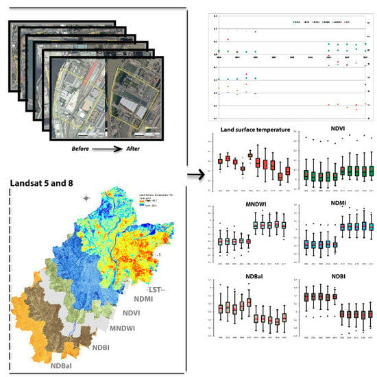
The objective of the study is to compare the evolution of the surface temperature of the main developments in Lyon with that of the spectral indices. To this end, a representative panel of vegetation, water, moisture, building, and bare-soil indices was tested at the four study sites (Table 3). However, not all these spectral indices are equally effective, depending on the nature and morphological parameters of the study site. Selection based on theoretical benefits from the literature and practical application at the sites made it possible to select an index for each type of variable: NDVI for vegetation, MNDWI for water, NDMI for humidity, NDBI for buildings, and NDBaI for bare soil (Figure 6).
In addition, the Urban Thermal Field Variance Index (UTFVI) was calculated for each site. The UTFVI can be used to quantitatively analyze the UHI effect and be divided into six levels, in line with six specific ecological evaluation indices (Table 4 and Figure 7). It can be calculated with Equation (14):
where Ts is the LST of a pixel (°C or °K), and Tmean is the mean LST of the whole study area (°C or °K).
2.6. Trend and Break Analysis
Comparisons of the selected indices for each site before and after redevelopment were evaluated using the Wilcoxon signed rank test [93] (matched samples, non-Gaussian distributions tested using the Shapiro–Wilk test. This test is well-suited for samples with fewer than 5000 observations [94]). The Pettitt [47] and SNHT tests [48] were used to examine if a series can be considered homogeneous over time or if there is a time at which a lag occurs, for example, at the time of accommodation. These homogeneity tests are nonparametric tests that do not require any assumptions about data distribution. The tests can be used on variables with any distribution. Finally, trends are characterized using the Mann–Kendall test on indicator medians [95]. The absence of autocorrelation in the series was checked using the autocorrelation function [96].
3. Results
3.1. Confluence Site
The Confluence site was transformed from an industrial site to a tertiary and residential area. This led to major urban changes impacting the average temperature of the site. Indeed, since the changes have taken place, median LST decreased by about 4 °C (Figure 8 and Figure 9, and Table 5). This decrease was confirmed by the Wilcoxon signed rank test, the Pettitt test, the SNHT, and the Mann–Kendall trend test. The same is valid for the UTFVI. This change in surface temperature is related to the change in land use and land cover (LULC), as evidenced by the results of the spectral indices. The NDVI, NDMI, and MNDWI experienced significant increases, while the NDBI and NDBaI have decreasing values due to the developments (Table 5).
3.2. Kaplan Park
Similarly to Confluence, Jacob Kaplan Park is located on former brownfield land. The Wilcoxon signed rank and SNHT tests indicated a decrease in surface temperature related to changes in land use (Table 6). In addition, all tests indicated a decrease in UTFVI. The spectral indices of vegetation, moisture, and water increased, unlike the building and bare-soil indices, which decreased.
3.3. Museum Site
Like the previous two sites, the museum site was built on a former industrial site. However, and in contrast to the two previous sites, LST did not have a decreasing trend but remained stable, of the exception of the Wilcoxon test, which indicates an increase. The NDVI and NDBaI did not show a net change either except for the Wilcoxon test, which showed a decrease (Table 7). On the contrary, the NDBI is decreasing for all the tests performed, unlike the NDMI and MNDWI.
3.4. Dock Site
The results on the dock site indicate no change in either the surface temperature or the UTFVI, except for the Wilcoxon signed rank test, which indicated an increase (Table 8). The same is true for the NDVI and NDBaI, showing no change. In addition, all tests indicate a decrease in NDBI, including a Kendall rate of −0.5. Conversely, the NDMI and MNDWI increased (Table 8).
3.5. Garibaldi Street
On the Garibaldi site, the results are similar to those of the dock site: no change in LST and UTFVI (except for the Wilcoxon signed rank test, which indicated a difference), NDVI, and NDBaI. It also showed a decrease in NDBI and an increase in NDMI and MNDWI (Table 9).
3.6. Groupama Stadium
Unlike the previous sites, Groupama Stadium was built on cereal or wooded agricultural land, free of any pre-existing buildings. We saw an increase in LST and UTFVI, with a decrease in NDVI. For the NDBI, NDBaI, and NDMI, the Pettitt, SNHT, and Mann–Kendall tests did not show any change, unlike the Wilcoxon test, which showed a decrease in building and bare-soil areas, and an increase in moisture content. The tests indicate an increase in MNDWI, with values that, however, remained negative (Table 10).
4. Discussion
The results highlight two distinct site configurations: requalifications that integrate vegetation and a consequent water supply with a decrease in surface temperatures (Confluence and Kaplan), and developments that focus less on environmental quality but more on the development itself, with a stagnation of surface temperatures (Museum, dock, and Garibaldi Street), or even an increase (Groupama Stadium). Indeed, a decrease in surface temperature was observed at the Confluence and Kaplan sites, validated by the Wilcoxon and SNHT tests. In addition, the Pettitt and Mann–Kendall trends confirm this decrease for the Confluence site (Table 5 and Table 6). A similar decrease can be observed for UTFVI. For example, before its redesign, Confluence’s UTFVI oscillated around 0.15 (e.g., 0.23 in 2001, 0.21 in 2002, 0.15 in 2005), representative of a stronger urban heat island phenomenon (Table 5). After redevelopment, the UTFVI fell below 0.05, sometimes even with negative values (−0.02 in 2015 and −0.01 in 2017), representative of a low ICU and a good or excellent Ecological Evaluation Index (Table 5).
These results are in accordance with more significant changes on the site: vacant land areas with little or no vegetation gave way to grassed and wooded areas, associated with more humidity (Figure 2). Because of its revegetation, the NDVI and NDMI increased, as indicated by the four tests (Figure 10 and Figure 11). With regard to the MNDWI, there is also a positive variation following the transformation. Indeed, in the case of the Confluence site, a 2 ha water basin was dug (Figure 2). The dock explains the positive MNDWI values obtained after redevelopment, reflecting Landsat mesh pixels completely covered with water. For the Jacob Kaplan Park, a 540 m2 pool was also created. However, given the Landsat grid area of 900 m2, no positive value was obtained. The building (NDBI) and bare soil (NDBaI) indices, on the other hand, unsurprisingly decreased. (Figure 12 and Figure 13). Indeed, land-cover changes have largely been characterized by green spaces and water surfaces.
This transformation of the environment of these two sites was planned before redevelopment by country planners and promoters. In addition to the primary objective of converting these former industrial areas into tertiary or residential sectors, considerable attention has been paid to the living environment offered to residents and passers-by, with a large number of environmental amenities. However, a careful reading of the development projects in these areas indicates that the notion of thermal comfort in itself was not present in the urban-planning documents. However, it is possible to find development objectives in terms of limiting rainwater discharge into the sewerage network in order to minimize its overloading and prevent flooding. This was made possible by promoting infiltration at the source, particularly through valleys or water gardens (Figure 14). These developments linked to rainwater infiltration are therefore initially intended to fight against flooding and massive waterproofing. However, they have a secondary role in combating heat in urban areas, although this was not present in the minds of planners. Indeed, even in summer, these oases of greenery provide freshness and shade to the surrounding areas.
The Confluence and Kaplan major transformations required several million euros of investment over several years. They led to a decrease in surface temperature following the creation of water areas and vegetated areas in place of asphalt surfaces and brownfields. This was followed by increases in the NDVI and NDMI, combined with decreases in the NDBI and NDBaI. In addition to improving the environment, they helped change the image of the neighborhood. Indeed, until the mid-2000s, the Confluence district had a very negative reputation. It was the location of the wholesale market, as well as Saint Paul and Saint Joseph, two prisons that were built in the 19th century south of Perrache station. In addition, the neighborhood was very much affected by prostitution. In 2009, the prisons were relocated to eastern Lyon. The historic buildings were renovated and are now used as premises for the Catholic University of Lyon. The wholesale market was also closed in 2009 and was also moved to eastern Lyon. Kaplan Park followed a similar progression as part of a broader redevelopment operation. Formerly made up of industrial wasteland after having been a site for the construction of railway equipment, the site is now the southern gateway to the Part-Dieu business district.
The situation is different when considering the dock, Garibaldi Street, and the Museum site. For these three sites, unlike the sites with more significant transformations, no change in surface temperature was observed, except by the Wilcoxon signed rank test, which indicated an increase for both sites (Table 7, Table 8 and Table 9). The same is true for the UTFVI. The explanation probably lies in the fact that these sites have been subject to minor instead of major redevelopments. On the dock, 2500 and 1600 m2 of asphalt were transformed into lawn and water, respectively, as evidenced by the increase in the MNDWI. However, 2800 m2 of gore (a type of sandy soil resulting from the decomposition of granite) was replaced by mainly grey stone (Figure 4). In addition, about ten tall trees in the south of the site were cut down and replaced by small shrubs that do not yet offer significant shaded vegetated areas (Figure 4). These reasons could explain the stagnation of surface temperature (Table 7) and NDVI (Figure 10), the decrease in NDBI (Figure 12), and the increase in NDMI (Figure 11). The NDBaI did not change because no bare soil was present at the time, just as in its current state (Figure 3 and Figure 13).
As with the dock and Garibaldi Street, results suggested that the surface temperatures at the Museum site were stable, except for the Wilcoxon test, which detected an increase (Table 7). The latter also detected a decrease in NDVI, NDBaI, and NDBI. The decrease in the NDBI was also confirmed by the other tests, which did not, however, find a trend for the NDVI and the NDBI. The stabilizations of the NDVI and NDBaI are not surprising: the vegetated areas and bare land areas did not really change during requalification (Figure 2). Before its requalification, the site had relatively few vegetated areas that were not really maintained. Following its redevelopment, the site does not really have any more vegetated surface. In addition, all high trees were cut down and replaced by herbaceous surfaces in which shrubs were planted, which do not yet offer significant shade. The NDBI decreased as a result of the decrease in built areas from 40,000 to 33,000 m2. In contrast, the NDMI experienced a significant increase according to all tests. This is linked to the intensive maintenance of green spaces and the installation of gore that retains moisture. The site of the Lyon Museum is a key place for the urban area, clearly visible from the main southern highway. Thus, site managers take care to offer an abundantly watered green space to visitors and passers-by.
In the context of Garibaldi Street, surface temperature did not change because, as on the dock, redevelopments were less significant than those at Confluence and at Kaplan Park (Table 8 and Figure 3). The urban highway was replaced by lighter modes of transport, road transport has been reduced, and coexistence between pedestrians, cyclists, and motorists has been facilitated. However, shrub cover has not considerably changed, as indicated by the stagnation of the NDVI (Figure 3 and Figure 10). Sustainable stormwater-management surface developments have emerged with the creation of valleys, which helps explain the increase in the NDMI (Figure 11) and the decrease in the NDBI (Figure 12). However, these developments are difficult to detect from the sky because of their small size, especially since they are located under the vegetative cover of taller trees (Figure 3). As on the dock site, the NDBaI did not change for similar reasons (Figure 13).
It appears that the light requalifications of these sites had no beneficial impact on surface temperature. On the contrary, an increase was even detected by the Wilcoxon test, thus reducing the thermal comfort of the inhabitants. This is evident when we specifically focus on the development of the docks. The century-old trees that produced wide shade in summer were cut down and replaced by bleachers of white stones and grey deactivated concrete (Figure 14). The trees that were planted there will not provide shade comparable to their predecessors for many years to come. In summer, this place has become very uncomfortable due to the very high heat and associated reverberation, especially since it is exposed to the west and south. It appears that the place is unattended by the population on summer afternoons.
The same applies to the square in front of the museum (Figure 2 and Figure 14). In addition to its cultural vocation, the main function of the redevelopment of the museum site was thus to ensure a communication and enhancement role for the image of the Lyon metropolis. Architects and local elected officials probably did not want trees to hide their creation. Consequently, the front square is composed of a 2000 m2 concrete area without any vegetation or shade. This results in extremely high temperatures on summer afternoons, providing major thermal discomfort, especially when people wishing to visit the museum have to queue for hours under the sun without any protection. In addition, tiny crystals are included in the concrete for purely aesthetic purposes, to make the ground sparkle. However, in summer, they strongly reflect the sun’s rays, which is extremely unpleasant for the eyes and increases thermal discomfort.
The results from the Groupama Stadium site show a significant increase in surface temperature and UTFVI (Table 10). Surface temperatures were already relatively high in summer on ploughed agricultural land, with average temperatures of 38.2 and 36.8 °C in July 2003 and June 2005, respectively. However, after the construction of the stadium, surface temperatures have been exceeding 40 °C, with, for example, 42.2°C in July 2013 and 42.3 °C in August 2015. According to the UTFVI, the urban heat island phenomenon was weak or better (−0.121 in 2002 and −0.009 in 2004 and 2005 for example) on the site before building the Stadium, but jumped to 0.096 in 2015 or 0.071 in 2016, meaning a stronger UHI, with the worst ecological evaluation index (Table 4 and Table 10). The stadium was built on agricultural and wooded land: this resulted in a decrease in the NDVI, which had high values before construction (0.315 in 2001; 0.491 in 2002), and now has much lower values (0.087 in 2014; 0.190 in 2017). On the other hand, the NDMI increased for the Wilcoxon test. This can be explained by the fact that the site was overwhelmingly occupied by agricultural land before the stadium was built. In the middle of summer, these lands had very low NDMI values after harvests (−0.213 in 2003; −0.278 in 2004). These agricultural fields have been replaced by football fields that require abundant watering in summer. This results in higher overall NDMI values, especially since the training grounds have been fully used in recent years (0.032 in 2016; 0.016 in 2017). The decrease in the NDBI for the Wilcoxon test in particular is more counterintuitive (0.213 in 2003; 0.024 in 2014; −0.032 in 2016). Similarly, the increase in the MNDWI, confirmed by all the tests, may seem surprising in view of the developments carried out in the area (−0.456 in 2001; −0.372 in 2005; −0.164 in 2015). These are the limitations of these indicators, which are discussed in more detail in the section on the study’s uncertainties and limitations.
The objective of the redevelopment of the Groupama Stadium site is different from the work carried out on the other sites. Indeed, on the other five sites, the objective was to redevelop old obsolete sites where the natural environment was more constrained than accepted, and not at all enhanced. The redevelopment of these sites has thus allowed the return of more natural habitats, with additional wetness, even if the objective of reducing heat stress was not clearly identified. This resulted in the opposite results on surface temperature, depending on the nature of the work and the developments that took place. However, changes in the sites’ function were not as abrupt as for the Groupama Stadium. Indeed, in this case, land use was totally modified because the sports complex was built on agricultural and wooded land. This has resulted in an overall decrease in vegetation, an increase in surface temperature, and a decrease in biodiversity. As this place is only frequented by the population during matches or concerts, the problem of heat stress seems to be less problematic than for the museum, dock, and Garibaldi Street sites, especially since the events generally take place in the evening, during lower temperatures. Nevertheless, the construction of the stadium did have a local impact on the surrounding thermal environment, which in a way contributes to the overall increase in the urban heat island of Lyon.
The work presented in this article is innovative since it focuses on the impact of site redevelopment on surface temperature and its environment over a period of about fifteen years, taking into account the initial state of the site until it is completely transformed and after a few years of use. Nevertheless, this work has some limitations related to various factors that we now discuss.
Changes in surface temperatures and humidity have been highlighted. However, these changes are only perceived through satellite data, with a 30 m mesh, and all the limitations inherent in this type of data. Thus, it would have been very interesting to be able to benefit from ground measurements, particularly of temperature and humidity, in order to compare the two means of measuring parameters. However, no measurements were available. The Greater Lyon area suffers from a total lack of a ground-temperature measurement network, despite our repeated requests to the city’s engineers, although it was equipped with rain gauges for some 20 years. This comparison is thus one of the possibilities of this work. Indeed, mobile temperature and humidity measurements are currently being carried out by us, synchronous with the passage of Landsat.
Secondly, the surface temperature or air temperature does not directly reflect thermal comfort. Indeed, the latter depends on other parameters such as humidity, radiation, insolation or wind speed. To evaluate thermal comfort, several indices were proposed, such as the thermohygrometric index [97], the heat index [32,98], and the Universal Thermal Climate Index [99,100]. These quantitative indices can be combined with more qualitative approaches, such as commented paths [22,23]. A study of this kind is currently underway in Lyon, with the participation of visually impaired people.
In addition, the requalification study sites have different sizes: Kaplan 6000 m2, Garibaldi Street 14,500 m2, dock 20,000 m2, museum 42,900 m2, and Confluence 170,000 m2 (Groupama Stadium with its 550,000 m2 is a special case given its construction on mainly agricultural land). The study sites are relative to a dense Western European metropolitan area. Confluence remains one of the largest redevelopment projects in Lyon. In addition, the results of the impact of redevelopment on surface temperature do not depend on site size, but on the type of facilities that are being deployed. Indeed, the two sites that had a positive impact on surface temperature were not the largest (Kaplan and Confluence) but those that have been most profoundly transformed, with significant vegetation changes and an increase in humid/water surfaces. It is therefore necessary for developers to take into account the nature of the work and to know that even a relatively small site, for example, less than 10,000 m2, could have a positive impact on local UHIs. Though each redevelopment project is unique, the results can be applicable to areas other than just those studied depending on the types of redevelopments.
Within the framework of this study, six sites in the Lyon metropolitan area were studied. The choice of these sites was determined by the scope and type of redevelopment, but also by the study period. Indeed, the redevelopment had to take place between the mid-2000s and early 2010 in order to be able to study the initial and final conditions of each of the sites. As the results showed, the impacts are dependent on the type of the redevelopment carried out, and not on the size of the sites. Thus, the impact of each redevelopment is specific, and the multiplication of the number of sites may not be essential.
The different surface temperatures and spectral indices were calculated using Landsat 5 before the developments took place, and with Landsat 8 afterward. The wavelengths of the different bands changed very slightly, with Landsat 8 being slightly narrower, but changes remained small and were not likely to affect the results (for example, the red band of Landsat 5 was 0.63–0.69 µm, and that of Landsat was 0.64–0.67 µm). Another limitation related to the satellite data is in the study grid. As mentioned in Section 2.4, thermal strips were at 30 m resolution in the delivered data product after resampling. However, in urban areas, the diversity of land use means that there is a high diversity of materials in a mesh. This weakens the spectral signal. A solution would be to carry out measurements that would acquire high-resolution urban land-surface temperature data (e.g., 7 m/pixel) [8,41]. Finally, there are several algorithms for calculating surface temperature, as mentioned in Section 2.4, and a comparison of the different results at the sites would be interesting, although the results should probably be very close [101].
As explained in Section 2.5, a selection of spectral indices was picked. For example, for the vegetation study, the effectiveness of four indices was evaluated from the literature and site application (NDVI, SAVI, EVI, and GVI), and the NDVI was selected for this study. Nevertheless, trends in the other indices were also analyzed and the results are consistent with those used, with the exception of the NDWI. Indeed, the latter is “often mixed with built-up land noise and the area of extracted water is thus overestimated” [88].
In addition, the spectral indices themselves could have weaknesses. For example, although the use of MNDWI is preferable to NDWI [102], some pixels that were identified as water were not in reality. This is especially the case in the eastern part of the urban area and does not concern the studied sites (Figure 6). Concerning the NDBI and, as mentioned above on the Groupama Stadium site, (only) the Wilcoxon test indicated a decrease in the number of built areas. This cannot be the case because the stadium was built on agricultural and wooded land. This is a limitation of the indicator itself that presents difficulties in separating constructed and bare ground due to the high complexity of spectral-response patterns [91,103]. Another limitation may be related to the NDBaI, which has problems “to distinguish cultivated areas and urban areas where an urban heat island is serious” [104].
5. Conclusions
The study showed that heavy redevelopments are required to achieve a decrease in surface temperature, and that the results are not related to the size of the site. This essentially involves reducing the number of artificial surfaces and greening the space. In this sense, the transformations of the Confluence and Kaplan Park sites are truly successful. The lighter redevelopments do not seem to significantly change the intensity of surface temperatures. On the contrary, the Wilcoxon signed rank test indicated an increase in the latter for the dock or Garibaldi Street sites, as for the museum and the Groupama Stadium. However, the purpose of these developments was not intentionally related to their impact on surface temperature, and they still fulfilled their role with improved stormwater management, or the replacement of parking lots with green spaces on the dock, among many other measures. However, planners should keep in mind the notion of thermal comfort and systematically take into account the temperature factor in their planning operations. In addition, the integration of natural spaces structures the district, strengthens the link with nature, and improves the quality of life of the inhabitants.
In the meantime, it should not be forgotten that this is a study mainly concerned with the measurement of surface temperature by remote sensing. However, as mentioned above, it does not systematically reflect the air temperature physically sensed by the inhabitants. Ground-based measurements of air temperature and humidity before and after the redevelopments would therefore have been useful to compare to the measurements obtained by remote sensing. As a result of the present study, discussions with Lyon’s urban planners have raised awareness, and they are trying to equip redevelopment sites with meteorological sensors when the financial and material conditions allow for it.
Author Contributions
Conceptualization, F.R. and L.A.; methodology, F.R., L.A., and Y.F.; validation, Y.F., J.C. and A.H.; formal analysis, F.R., L.A., and Y.F.; writing—original draft preparation, F.R. and L.A.; writing—review and editing, F.R., L.A., Y.F., and A.H.; supervision, J.C.; project administration, F.R.
Funding
This work is part of the 3M’Air project, performed within the framework of the LABEX IMU (ANR-10-LABX-0088) of Université de Lyon, within the program “Investissements d’Avenir” (ANR-11-IDEX-0007) operated by the French National Research Agency (ANR).
Acknowledgments
The authors gratefully acknowledge USGS NASA, Météo-France, and the Lyon Metropolis for the useful data, free of charge. This work would not have been possible without it. The authors wish to thank the four reviewers who helped a lot to improve the quality the text.
Conflicts of Interest
The authors declare no conflict of interest.
References
- Core Writing Team; Pachauri, R.K.; Meyer, L.A. (Eds.) IPCC, 2014: Climate Change 2014: Synthesis Report. Contribution of Working Groups I, II and III to the Fifth Assessment Report of the Intergovernmental Panel on Climate Change; IPCC: Geneva, Switzerland, 2014. [Google Scholar]
- Della-Marta, P.M.; Haylock, M.R.; Luterbacher, J.; Wanner, H. Doubled length of western European summer heat waves since 1880. J. Geophys. Res. Atmos. 2007, 112. [Google Scholar] [CrossRef]
- Fink, A.H.; Brücher, T.; Krüger, A.; Leckebusch, G.C.; Pinto, J.G.; Ulbrich, U. The 2003 European summer heatwaves and drought–synoptic diagnosis and impacts. Weather 2004, 59, 209–216. [Google Scholar] [CrossRef]
- Weston, K.J. Boundary Layer Climates, 2nd ed.; Methuen, T.R.O., Ed.; Psychology Press: London, UK, 1987; pp. 435 + xvi. [Google Scholar]
- Huang, Q.; Lu, Y. Urban heat island research from 1991 to 2015: A bibliometric analysis. Theor. Appl. Climatol. 2018, 131, 1055–1067. [Google Scholar] [CrossRef]
- Xian, G.; Crane, M. An analysis of urban thermal characteristics and associated land cover in Tampa Bay and Las Vegas using Landsat satellite data. Remote Sens. Environ. 2006, 104, 147–156. [Google Scholar] [CrossRef]
- Bohnenstengel, S.I.; Evans, S.; Clark, P.A.; Belcher, S.E. Simulations of the London urban heat island. Q. J. R. Meteorol. Soc. 2011, 137, 1625–1640. [Google Scholar] [CrossRef]
- Sobrino, J.A.; Oltra-Carrió, R.; Sòria, G.; Jiménez-Muñoz, J.C.; Franch, B.; Hidalgo, V.; Mattar, C.; Julien, Y.; Cuenca, J.; Romaguera, M.; et al. Evaluation of the surface urban heat island effect in the city of Madrid by thermal remote sensing. Int. J. Remote Sens. 2013, 34, 3177–3192. [Google Scholar] [CrossRef]
- Azevedo, J.A.; Chapman, L.; Muller, C.L. Quantifying the Daytime and Night-Time Urban Heat Island in Birmingham, UK: A Comparison of Satellite Derived Land Surface Temperature and High Resolution Air Temperature Observations. Remote Sens. 2016, 8, 153. [Google Scholar] [CrossRef]
- Martin, P.; Baudouin, Y.; Gachon, P. An alternative method to characterize the surface urban heat island. Int. J. Biometeorol. 2015, 59, 849–861. [Google Scholar] [CrossRef] [PubMed]
- Voogt, J.A.; Oke, T.R. Thermal remote sensing of urban climates. Remote Sens. Environ. 2003, 86, 370–384. [Google Scholar] [CrossRef]
- Walawender, J.P.; Szymanowski, M.; Hajto, M.J.; Bokwa, A. Land Surface Temperature Patterns in the Urban Agglomeration of Krakow (Poland) Derived from Landsat-7/ETM+ Data. Pure Appl. Geophys. 2014, 171, 913–940. [Google Scholar] [CrossRef]
- Zhou, D.; Xiao, J.; Bonafoni, S.; Berger, C.; Deilami, K.; Zhou, Y.; Frolking, S.; Yao, R.; Qiao, Z.; Sobrino, J.A. Satellite Remote Sensing of Surface Urban Heat Islands: Progress, Challenges, and Perspectives. Remote Sens. 2019, 11, 48. [Google Scholar] [CrossRef]
- Qaid, A.; Lamit, H.B.; Ossen, D.R.; Rasidi, M.H. Effect of the position of the visible sky in determining the sky view factor on micrometeorological and human thermal comfort conditions in urban street canyons. Theor. Appl. Climatol. 2018, 131, 1083–1100. [Google Scholar] [CrossRef]
- Lin, P.; Lau, S.S.Y.; Qin, H.; Gou, Z. Effects of urban planning indicators on urban heat island: A case study of pocket parks in high-rise high-density environment. Landsc. Urban Plan. 2017, 168, 48–60. [Google Scholar] [CrossRef]
- Keeratikasikorn, C.; Bonafoni, S. Urban Heat Island Analysis over the Land Use Zoning Plan of Bangkok by Means of Landsat 8 Imagery. Remote Sens. 2018, 10, 440. [Google Scholar] [CrossRef]
- Fung, W.Y.; Lam, K.S.; Nichol, J.; Wong, M.S. Derivation of Nighttime Urban Air Temperatures Using a Satellite Thermal Image. J. Appl. Meteor. Climatol. 2009, 48, 863–872. [Google Scholar] [CrossRef]
- Liu, L.; Lin, Y.; Wang, D.; Liu, J. An improved temporal correction method for mobile measurement of outdoor thermal climates. Theor. Appl. Climatol. 2017, 129, 201–212. [Google Scholar] [CrossRef]
- Yu, X.; Guo, X.; Wu, Z. Land Surface Temperature Retrieval from Landsat 8 TIRS—Comparison between Radiative Transfer Equation-Based Method, Split Window Algorithm and Single Channel Method. Remote Sens. 2014, 6, 9829–9852. [Google Scholar] [CrossRef]
- Shohei, K.; Takeki, I.; Hideo, T. Relationship between Terra/ASTER Land Surface Temperature and Ground-observed Air Temperature. Geogr. Rev. Jpn. B 2016, 88, 38–44. [Google Scholar] [CrossRef]
- Lin, T.-P. Thermal perception, adaptation and attendance in a public square in hot and humid regions. Build. Environ. 2009, 44, 2017–2026. [Google Scholar] [CrossRef]
- Makaremi, N.; Salleh, E.; Jaafar, M.Z.; GhaffarianHoseini, A. Thermal comfort conditions of shaded outdoor spaces in hot and humid climate of Malaysia. Build. Environ. 2012, 48, 7–14. [Google Scholar] [CrossRef]
- Yang, W.; Wong, N.H.; Jusuf, S.K. Thermal comfort in outdoor urban spaces in Singapore. Build. Environ. 2013, 59, 426–435. [Google Scholar] [CrossRef]
- Kovats, R.S.; Hajat, S. Heat stress and public health: A critical review. Annu. Rev. Public Health 2008, 29, 41–55. [Google Scholar] [CrossRef] [PubMed]
- Smargiassi, A.; Goldberg, M.S.; Plante, C.; Fournier, M.; Baudouin, Y.; Kosatsky, T. Variation of daily warm season mortality as a function of micro-urban heat islands. J. Epidemiol. Community Health 2009, 63, 659–664. [Google Scholar] [CrossRef] [PubMed]
- Nayak, S.G.; Shrestha, S.; Kinney, P.L.; Ross, Z.; Sheridan, S.C.; Pantea, C.I.; Hsu, W.H.; Muscatiello, N.; Hwang, S.A. Development of a heat vulnerability index for New York State. Public Health 2017, 161, 127–137. [Google Scholar] [CrossRef] [PubMed]
- Robine, J.-M.; Cheung, S.L.K.; Le Roy, S.; Van Oyen, H.; Griffiths, C.; Michel, J.-P.; Herrmann, F.R. Death toll exceeded 70,000 in Europe during the summer of 2003. C. R. Biol. 2008, 331, 171–178. [Google Scholar] [CrossRef] [PubMed]
- Laaidi, K.; Zeghnoun, A.; Dousset, B.; Bretin, P.; Vandentorren, S.; Giraudet, E.; Beaudeau, P. The Impact of Heat Islands on Mortality in Paris during the August 2003 Heat Wave. Environ. Health Perspect 2012, 120, 254–259. [Google Scholar] [CrossRef] [PubMed]
- Vandentorren, S.; Bretin, P.; Zeghnoun, A.; Mandereau-Bruno, L.; Croisier, A.; Cochet, C.; Ribéron, J.; Siberan, I.; Declercq, B.; Ledrans, M. August 2003 heat wave in France: Risk factors for death of elderly people living at home. Eur. J. Public Health 2006, 16, 583–591. [Google Scholar] [CrossRef] [PubMed]
- Dousset, B.; Gourmelon, F.; Laaidi, K.; Zeghnoun, A.; Giraudet, E.; Bretin, P.; Mauri, E.; Vandentorren, S. Satellite monitoring of summer heat waves in the Paris metropolitan area. Int. J. Climatol. 2011, 31, 313–323. [Google Scholar] [CrossRef]
- State of World Population 2007. Available online: www.unfpa.org/fr/node/5923 (accessed on 17 July 2018).
- Desai, M.S.; Dhorde, A.G. Trends in thermal discomfort indices over western coastal cities of India. Theor. Appl. Climatol. 2018, 131, 1305–1321. [Google Scholar] [CrossRef]
- Wicki, A.; Parlow, E.; Wicki, A.; Parlow, E. Multiple Regression Analysis for Unmixing of Surface Temperature Data in an Urban Environment. Remote Sens. 2017, 9, 684. [Google Scholar] [CrossRef]
- Wang, J.; Zhan, Q.; Guo, H. The Morphology, Dynamics and Potential Hotspots of Land Surface Temperature at a Local Scale in Urban Areas. Remote Sens. 2016, 8, 18. [Google Scholar] [CrossRef]
- Tomlinson, C.J.; Chapman, L.; Thornes, J.E.; Baker, C.J. Derivation of Birmingham’s summer surface urban heat island from MODIS satellite images. Int. J. Climatol. 2012, 32, 214–224. [Google Scholar] [CrossRef]
- Benas, N.; Chrysoulakis, N.; Cartalis, C. Trends of urban surface temperature and heat island characteristics in the Mediterranean. Theor. Appl. Climatol. 2017, 130, 807–816. [Google Scholar] [CrossRef]
- dos Santos, A.R.; de Oliveira, F.S.; da Silva, A.G.; Gleriani, J.M.; Gonçalves, W.; Moreira, G.L.; Silva, F.G.; Branco, E.R.F.; Moura, M.M.; da Silva, R.G.; et al. Spatial and temporal distribution of urban heat islands. Sci. Total Environ. 2017, 605–606, 946–956. [Google Scholar] [CrossRef] [PubMed]
- Sugawara, H.; Shimizu, S.; Takahashi, H.; Hagiwara, S.; Narita, K.; Mikami, T.; Hirano, T. Thermal Influence of a Large Green Space on a Hot Urban Environment. J. Environ. Qual. 2016, 45, 125–133. [Google Scholar] [CrossRef] [PubMed]
- Masoudi, M.; Tan, P.Y. Multi-year comparison of the effects of spatial pattern of urban green spaces on urban land surface temperature. Landsc. Urban Plan. 2019, 184, 44–58. [Google Scholar] [CrossRef]
- Liu, H.; Zhan, Q.; Yang, C.; Wang, J. Characterizing the Spatio-Temporal Pattern of Land Surface Temperature through Time Series Clustering: Based on the Latent Pattern and Morphology. Remote Sens. 2018, 10, 654. [Google Scholar] [CrossRef]
- Jenerette, G.D.; Harlan, S.L.; Buyantuev, A.; Stefanov, W.L.; Declet-Barreto, J.; Ruddell, B.L.; Myint, S.W.; Kaplan, S.; Li, X. Micro-scale urban surface temperatures are related to land-cover features and residential heat related health impacts in Phoenix, AZ USA. Landsc. Ecol 2016, 31, 745–760. [Google Scholar] [CrossRef]
- Liu, L.; Zhang, Y. Urban Heat Island Analysis Using the Landsat TM Data and ASTER Data: A Case Study in Hong Kong. Remote Sens. 2011, 3, 1535–1552. [Google Scholar] [CrossRef]
- Roşca, C.F.; Harpa, G.V.; Croitoru, A.-E.; Herbel, I.; Imbroane, A.M.; Burada, D.C. The impact of climatic and non-climatic factors on land surface temperature in southwestern Romania. Theor. Appl. Climatol. 2017, 130, 775–790. [Google Scholar] [CrossRef]
- Chen, Y.; Quan, J.; Zhan, W.; Guo, Z. Enhanced Statistical Estimation of Air Temperature Incorporating Nighttime Light Data. Remote Sens. 2016, 8, 656. [Google Scholar] [CrossRef]
- Tran, H.; Uchihama, D.; Ochi, S.; Yasuoka, Y. Assessment with satellite data of the urban heat island effects in Asian mega cities. Int. J. Appl. Earth Obs. Geoinf. 2006, 8, 34–48. [Google Scholar] [CrossRef]
- Sen, P.K. Estimates of the Regression Coefficient Based on Kendall’s Tau. J. Am. Stat. Assoc. 1968, 63, 1379–1389. [Google Scholar] [CrossRef]
- Pettitt, A.N. A Non-Parametric Approach to the Change-Point Problem. J. R. Stat. Soc. Ser. C 1979, 28, 126–135. [Google Scholar] [CrossRef]
- Alexandersson, H. A homogeneity test applied to precipitation data. J. Climatol. 1986, 6, 661–675. [Google Scholar] [CrossRef]
- Buishand, T.A. Some Methods for Testing the Homogeneity of Rainfall Records. J. Hydrol. 1982, 58, 11–27. [Google Scholar] [CrossRef]
- Neumann, J. von Distribution of the Ratio of the Mean Square Successive Difference to the Variance. Ann. Math. Statist. 1941, 12, 367–395. [Google Scholar] [CrossRef]
- Barsi, J.A.; Lee, K.; Kvaran, G.; Markham, B.L.; Pedelty, J.A. The Spectral Response of the Landsat-8 Operational Land Imager. Remote Sens. 2014, 6, 10232–10251. [Google Scholar] [CrossRef]
- Barsi, J.A.; Schott, J.R.; Hook, S.J.; Raqueno, N.G.; Markham, B.L.; Radocinski, R.G. Landsat-8 Thermal Infrared Sensor (TIRS) Vicarious Radiometric Calibration. Remote Sens. 2014, 6, 11607–11626. [Google Scholar] [CrossRef]
- Montanaro, M.; Gerace, A.; Lunsford, A.; Reuter, D. Stray Light Artifacts in Imagery from the Landsat 8 Thermal Infrared Sensor. Remote Sens. 2014, 6, 10435–10456. [Google Scholar] [CrossRef]
- Gerace, A.; Montanaro, M. Derivation and validation of the stray light correction algorithm for the thermal infrared sensor onboard Landsat 8. Remote Sens. Environ. 2017, 191, 246–257. [Google Scholar] [CrossRef]
- Li, S.; Zhao, Z.; Miaomiao, X.; Wang, Y. Investigating spatial non-stationary and scale-dependent relationships between urban surface temperature and environmental factors using geographically weighted regression. Environ. Model. Softw. 2010, 25, 1789–1800. [Google Scholar] [CrossRef]
- Jimenez-Munoz, J.C.; Cristobal, J.; Sobrino, J.A.; Soria, G.; Ninyerola, M.; Pons, X.; Pons, X. Revision of the Single-Channel Algorithm for Land Surface Temperature Retrieval from Landsat Thermal-Infrared Data. IEEE Trans. Geosci. Remote Sens. 2009, 47, 339–349. [Google Scholar] [CrossRef]
- Sobrino, J.A.; Jiménez-Muñoz, J.C.; Paolini, L. Land surface temperature retrieval from LANDSAT TM 5. Remote Sens. Environ. 2004, 90, 434–440. [Google Scholar] [CrossRef]
- Jiménez-Muñoz, J.C.; Sobrino, J.A. A generalized single-channel method for retrieving land surface temperature from remote sensing data. J. Geophys. Res. Atmos. 2003, 108. [Google Scholar] [CrossRef]
- Qin, Z.; Karnieli, A.; Berliner, P. A mono-window algorithm for retrieving land surface temperature from Landsat TM data and its application to the Israel-Egypt border region. Int. J. Remote Sens. 2001, 22, 3719–3746. [Google Scholar] [CrossRef]
- Using the USGS Landsat Level-1 Data Product | Landsat Missions. Available online: https://landsat.usgs.gov/using-usgs-landsat-8-product (accessed on 14 August 2018).
- Markham, B.L.; Barker, J.L. Landsat MSS and TM Post-Calibration Dynamic Ranges, Exoatmospheric Reflectances and At-Satellite Temperatures; EOSAT Landsat Technical Notes 1; NASA/GSFC: Greenbelt, MD, USA, 1986; pp. 3–8. [Google Scholar]
- Peres, L.F.; DaCamara, C.C. Emissivity maps to retrieve land-surface temperature from MSG/SEVIRI. IEEE Trans. Geosci. Remote Sens. 2005, 43, 1834–1844. [Google Scholar] [CrossRef]
- Wan, Z.; Li, Z.-L. A physics-based algorithm for retrieving land-surface emissivity and temperature from EOS/MODIS data. IEEE Trans. Geosci. Remote Sens. 1997, 35, 980–996. [Google Scholar]
- Griend, A.A.V.D.; Owe, M. On the relationship between thermal emissivity and the normalized difference vegetation index for natural surfaces. Int. J. Remote Sens. 1993, 14, 1119–1131. [Google Scholar] [CrossRef]
- Sobrino, J.A.; Raissouni, N. Toward remote sensing methods for land cover dynamic monitoring: Application to Morocco. Int. J. Remote Sens. 2000, 21, 353–366. [Google Scholar] [CrossRef]
- Dash, P.; Göttsche, F.-M.; Olesen, F.-S.; Fischer, H. Separating surface emissivity and temperature using two-channel spectral indices and emissivity composites and comparison with a vegetation fraction method. Remote Sens. Environ. 2005, 96, 1–17. [Google Scholar] [CrossRef]
- Dash, P.; Göttsche, F.-M.; Olesen, F.-S.; Fischer, H. Land surface temperature and emissivity estimation from passive sensor data: Theory and practice-current trends. Int. J. Remote Sens. 2002, 23, 2563–2594. [Google Scholar] [CrossRef]
- Sobrino, J.A.; Raissouni, N.; Li, Z.-L. A Comparative Study of Land Surface Emissivity Retrieval from NOAA Data. Remote Sens. Environ. 2001, 75, 256–266. [Google Scholar] [CrossRef]
- Sobrino, J.A.; Jiménez-Muñoz, J.C.; Sòria, G.; Romaguera, M.; Guanter, L.; Moreno, J.; Plaza, A.; Martínez, P. Land surface emissivity retrieval from different VNIR and TIR sensors. IEEE Trans. Geosci. Remote Sens. 2008, 46, 316–327. [Google Scholar] [CrossRef]
- Huete, A.R. A soil-adjusted vegetation index (SAVI). Remote Sens. Environ. 1988, 25, 295–309. [Google Scholar] [CrossRef]
- Huete, A.; Didan, K.; Miura, T.; Rodriguez, E.P.; Gao, X.; Ferreira, L.G. Overview of the radiometric and biophysical performance of the MODIS vegetation indices. Remote Sens. Environ. 2002, 83, 195–213. [Google Scholar] [CrossRef]
- Kauth, R.; Thomas, G. The Tasselled Cap—A Graphic Description of the Spectral-Temporal Development of Agricultural Crops as Seen by LANDSAT. In Proceedings of the Symposium on Machine Processing of Remotely Sensed Data, Purdue University, West Lafayette, IN, USA, 29 June–1 July 1976; pp. 41–51. [Google Scholar]
- Gao, B. NDWI—A normalized difference water index for remote sensing of vegetation liquid water from space. Remote Sens. Environ. 1996, 58, 257–266. [Google Scholar] [CrossRef]
- Zha, Y.; Gao, J.; Ni, S. Use of normalized difference built-up index in automatically mapping urban areas from TM imagery. Int. J. Remote Sens. 2003, 24, 583–594. [Google Scholar] [CrossRef]
- MODIS UCSB Emissivity Library. Available online: https://icess.eri.ucsb.edu/modis/EMIS/html/em.html (accessed on 23 October 2018).
- Données Métropolitaines du Grand Lyon. Available online: https://data.grandlyon.com/ (accessed on 23 October 2018).
- Carlson, T.N.; Ripley, D.A. On the relation between NDVI, fractional vegetation cover, and leaf area index. Remote Sens. Environ. 1997, 62, 241–252. [Google Scholar] [CrossRef]
- Sobrino, J.A.; Caselles, V.; Becker, F. Significance of the remotely sensed thermal infrared measurements obtained over a citrus orchard. ISPRS J. Photogramm. Remote Sens. 1990, 44, 343–354. [Google Scholar] [CrossRef]
- Barsi, J.A.; Schott, J.R.; Palluconi, F.D.; Hook, S.J. Validation of a web-based atmospheric correction tool for single thermal band instruments. In Proceedings of the Earth Observing Systems X, San Diego, CA, USA, 31 July–2 August 2005. [Google Scholar] [CrossRef]
- Barsi, J.A.; Barker, J.L.; Schott, J.R. An Atmospheric Correction Parameter Calculator for a single thermal band earth-sensing instrument. In Proceedings of the 2003 IEEE International Geoscience and Remote Sensing Symposium, Toulouse, France, 21–25 July 2003; Volume 5, pp. 3014–3016. [Google Scholar]
- Cristóbal, J.; Jiménez-Muñoz, J.C.; Sobrino, J.A.; Ninyerola, M.; Pons, X. Improvements in land surface temperature retrieval from the Landsat series thermal band using water vapor and air temperature. J. Geophys. Res. Atmos. 2009, 114, D08103. [Google Scholar] [CrossRef]
- Bannari, A.; Morin, D.; Bonn, F.; Huete, A.R. A review of vegetation indices. Remote Sens. Rev. 1995, 13, 95–120. [Google Scholar] [CrossRef]
- Chen, X.-L.; Zhao, H.-M.; Li, P.-X.; Yin, Z.-Y. Remote sensing image-based analysis of the relationship between urban heat island and land use/cover changes. Remote Sens. Environ. 2006, 104, 133–146. [Google Scholar] [CrossRef]
- Glenn, E.; Huete, A.; Nagler, P.; Nelson, S.; Glenn, E.P.; Huete, A.R.; Nagler, P.L.; Nelson, S.G. Relationship Between Remotely-sensed Vegetation Indices, Canopy Attributes and Plant Physiological Processes: What Vegetation Indices Can and Cannot Tell Us About the Landscape. Sensors 2008, 8, 2136–2160. [Google Scholar] [CrossRef]
- Crist, E.P.; Cicone, R.C. A Physically-Based Transformation of Thematic Mapper Data—The TM Tasseled Cap. IEEE Trans. Geosci. Remote Sens. 1984, GE-22, 256–263. [Google Scholar] [CrossRef]
- McFEETERS, S.K. The use of the Normalized Difference Water Index (NDWI) in the delineation of open water features. Int. J. Remote Sens. 1996, 17, 1425–1432. [Google Scholar] [CrossRef]
- Ji, L.; Zhang, L.; Wylie, B.K. Analysis of dynamic thresholds for the normalized difference water index. Photogramm. Eng. Remote Sens. 2009, 75, 11. [Google Scholar] [CrossRef]
- Xu, H. Modification of normalised difference water index (NDWI) to enhance open water features in remotely sensed imagery. Int. J. Remote Sens. 2006, 27, 3025–3033. [Google Scholar] [CrossRef]
- Rikimaru, A.; Roy, P.S.; Miyatake, S. Tropical forest cover density mapping. Trop. Ecol. 2002, 43, 39–47. [Google Scholar]
- Kawamura, M.; Jayamanna, S.; Tsujiko, Y. Relation Between Social and Environmental Conditions in Colombo. Sri Lanka and the Urban Index Estimated by Satellite Remote Sensing Data. In Proceedings of the XVIIIth ISPRS Congress Technical Commission VII: Resource and Environmental Monitoring, Vienna, Austria, 9–19 July 1996; Volume 31, pp. 321–326. [Google Scholar]
- As-syakur, A.R.; Adnyana, I.W.S.; Arthana, I.W.; Nuarsa, I.W.; As-syakur, A.R.; Adnyana, I.W.S.; Arthana, I.W.; Nuarsa, I.W. Enhanced Built-Up and Bareness Index (EBBI) for Mapping Built-Up and Bare Land in an Urban Area. Remote Sens. 2012, 4, 2957–2970. [Google Scholar] [CrossRef]
- Xu, H. A new index for delineating built-up land features in satellite imagery. Int. J. Remote Sens. 2008, 29, 4269–4276. [Google Scholar] [CrossRef]
- Wilcoxon, F. Individual Comparisons by Ranking Methods. Biom. Bull. 1945, 1, 80–83. [Google Scholar] [CrossRef]
- Shapiro, S.S.; Wilk, M.B. An analysis of variance test for normality (complete samples). Biometrika 1965, 591–611. [Google Scholar] [CrossRef]
- Mann, H.B. Nonparametric Tests Against Trend. Econometrica 1945, 13, 245–259. [Google Scholar] [CrossRef]
- Box, G.E.P.; Pierce, D.A. Distribution of Residual Autocorrelations in Autoregressive-Integrated Moving Average Time Series Models. J. Am. Stat. Assoc. 1970, 65, 1509–1526. [Google Scholar] [CrossRef]
- Thom, E.C. The Discomfort Index. Weatherwise 1959, 12, 57–61. [Google Scholar] [CrossRef]
- Rothfusz, L.P.; Headquarters, N.S.R. The Heat Index Equation (Or, More than You Ever Wanted to Know about Heat Index); National Oceanic and Atmospheric Administration, National Weather Service, Office of Meteorology: Fort Worth, TX, USA, 1990; Volume 9023.
- Fiala, D.; Havenith, G.; Bröde, P.; Kampmann, B.; Jendritzky, G. UTCI-Fiala multi-node model of human heat transfer and temperature regulation. Int. J. Biometeorol. 2012, 56, 429–441. [Google Scholar] [CrossRef]
- Rozbicka, K.; Rozbicki, T. Variability of UTCI index in South Warsaw depending on atmospheric circulation. Theor. Appl. Climatol. 2018, 133, 511–520. [Google Scholar] [CrossRef]
- Meng, X.; Cheng, J.; Zhao, S.; Liu, S.; Yao, Y. Estimating Land Surface Temperature from Landsat-8 Data using the NOAA JPSS Enterprise Algorithm. Remote Sens. 2019, 11, 155. [Google Scholar] [CrossRef]
- Singh, K.V.; Setia, R.; Sahoo, S.; Prasad, A.; Pateriya, B. Evaluation of NDWI and MNDWI for assessment of waterlogging by integrating digital elevation model and groundwater level. Geocarto Int. 2015, 30, 650–661. [Google Scholar] [CrossRef]
- He, C.; Shi, P.; Xie, D.; Zhao, Y. Improving the normalized difference built-up index to map urban built-up areas using a semiautomatic segmentation approach. Remote Sens. Lett. 2010, 1, 213–221. [Google Scholar] [CrossRef]
- Zhao, H.; Chen, X. Use of normalized difference bareness index in quickly mapping bare areas from TM/ETM+. In Proceedings of the 2005 IEEE International Geoscience and Remote Sensing Symposium, Seoul, Korea, 29 July 2005; Volume 3, pp. 1666–1668. [Google Scholar]
Figure 1.
Location map of the Lyon metropolis. (source: left: Natural Earth; top-right: BD alti IGN, Euro Boundary Map; bottom-right: orthophotography data, Grand Lyon).
Figure 1.
Location map of the Lyon metropolis. (source: left: Natural Earth; top-right: BD alti IGN, Euro Boundary Map; bottom-right: orthophotography data, Grand Lyon).

Figure 2.
Confluence (top), Kaplan Park (middle), and Museum sites in 2003 (left) and 2015 (right).

Figure 3.
Dock (top) and Garibaldi (bottom) sites in 2003 (left) and 2015 (right).

Figure 4.
Groupama Stadium site in 2003 (left) and 2017 (right).

Figure 5.
Land-surface temperature (LST) of Greater Lyon on 16 July 2017.

Figure 6.
NDBI, NDVI, NDBaI, and NDMI on 16 July 2017 in the Lyon urban area.

Figure 7.
UTFVI on 16 July 2017 in Lyon urban area.

Figure 8.
LST boxplots for the Confluence site (red cross: average; black dots: min and max values).
Figure 8.
LST boxplots for the Confluence site (red cross: average; black dots: min and max values).

Figure 9.
Median LST (right) and spectral indices (left) for the Confluence site.

Figure 10.
NDVI boxplots for the six sites: Confluence (top-left), Kaplan Park (top-right), dock (middle-left), Garibadi Street (middle-right), Museum (bottom-left), and Groupama Stadium (bottom-right); red cross: average; black dots: min and max values.
Figure 10.
NDVI boxplots for the six sites: Confluence (top-left), Kaplan Park (top-right), dock (middle-left), Garibadi Street (middle-right), Museum (bottom-left), and Groupama Stadium (bottom-right); red cross: average; black dots: min and max values.

Figure 11.
NDMI boxplots for the six sites: Confluence (top-left), Kaplan Park (top-right), dock (middle-left), Garibadi Street (middle-right), Museum (bottom-left), and Groupama Stadium (bottom-right); red cross: average; black dots: min and max values.
Figure 11.
NDMI boxplots for the six sites: Confluence (top-left), Kaplan Park (top-right), dock (middle-left), Garibadi Street (middle-right), Museum (bottom-left), and Groupama Stadium (bottom-right); red cross: average; black dots: min and max values.

Figure 12.
NDBI boxplots for the six sites: Confluence (top-left), Kaplan Park (top-right), dock (middle-left), Garibadi Street (middle-right), Museum (bottom-left), and Groupama Stadium (bottom-right); red cross: average; black dots: min and max values.
Figure 12.
NDBI boxplots for the six sites: Confluence (top-left), Kaplan Park (top-right), dock (middle-left), Garibadi Street (middle-right), Museum (bottom-left), and Groupama Stadium (bottom-right); red cross: average; black dots: min and max values.

Figure 13.
NDBaI boxplots for the six sites: Confluence (top-left), Kaplan Park (top-right), dock (middle-left), Garibadi street (middle-right), Museum (bottom-left), and Groupama Stadium (bottom-right); red cross: average; black dots: min and max values.
Figure 13.
NDBaI boxplots for the six sites: Confluence (top-left), Kaplan Park (top-right), dock (middle-left), Garibadi street (middle-right), Museum (bottom-left), and Groupama Stadium (bottom-right); red cross: average; black dots: min and max values.

Figure 14.
Left: Landscaping in Confluence for sustainable stormwater management (Laurence Danière/SPL Lyon Confluence, 2017); Middle: Dock bleachers made of white stone and deactivated concrete; Right: Square in front of the Confluence Museum, without any vegetation and shade (source: Quentin Lafont).


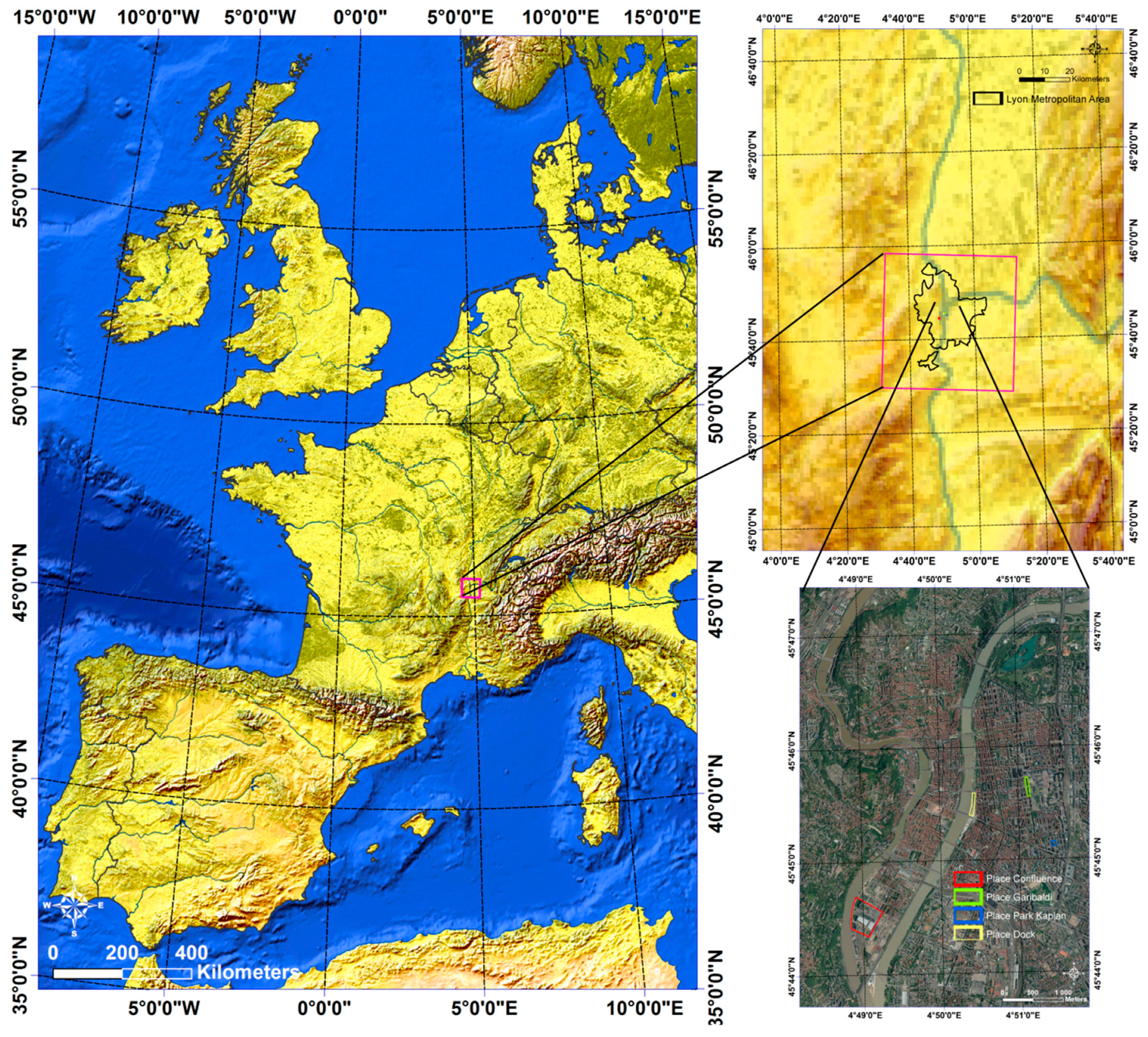
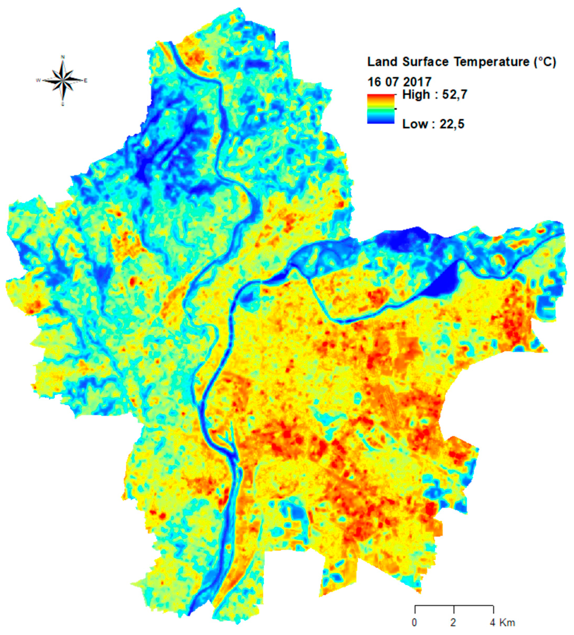
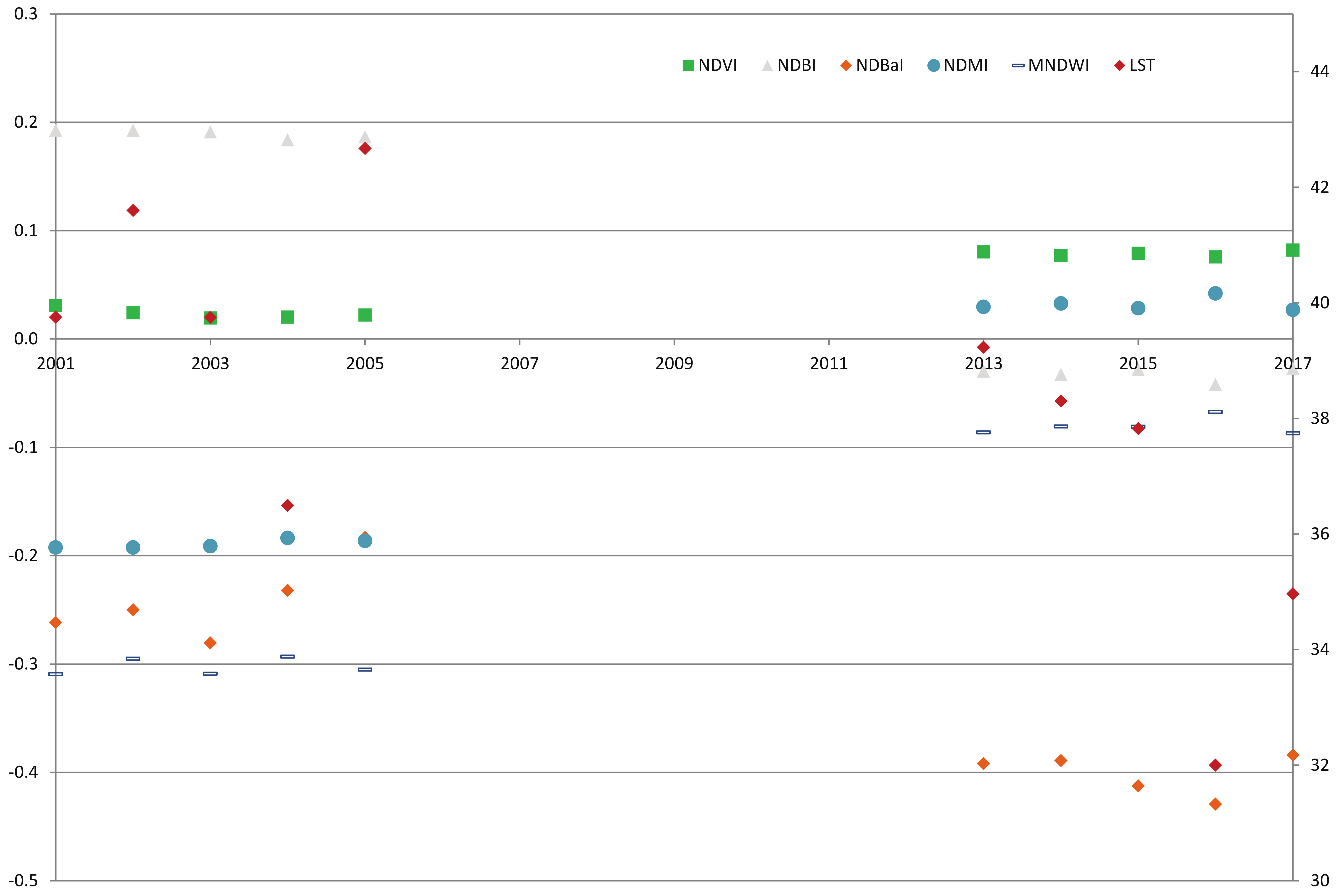
Table 1.
Meteorological parameters of study days at the Lyon-Bron station at 12:00 (source: Météo-France).
Table 1.
Meteorological parameters of study days at the Lyon-Bron station at 12:00 (source: Météo-France).
| 29 July 2001 | 14 June 2002 | 10 July 2003 | 21 July 2004 | 22 June 2005 | 21 July 2013 | 17 July 2014 | 05 Aug. 2015 | 23 Aug. 2016 | 16 July 2016 | |
|---|---|---|---|---|---|---|---|---|---|---|
| Temperature (°C) | 26.4 | 27.6 | 27.5 | 27.5 | 28.6 | 29.4 | 27.7 | 28.2 | 24.8 | 25.8 |
| Rain (mm) | 0 | 0 | 0 | 0 | 0 | 0 | 0 | 0 | 0 | 0 |
| Humidity (%) | 58 | 53 | 38 | 54 | 58 | 45 | 50 | 45 | 50 | 41 |
| Wind average (km/h) | 15 | 7 | 15 | 15 | 14 | 6 | 6 | 6 | 4 | 10 |
| Direction (°N) | 10 | 130 | 360 | 170 | 10 | 210 | 280 | 190 | 330 | 36 |
| Pressure (hPa) | 1021 | 1017.4 | 1017.6 | 1016.3 | 1019.1 | 1016.7 | 1018.9 | 1015.3 | 1024.4 | 1022.6 |
| Landsat satellite | 5 | 5 | 5 | 5 | 5 | 8 | 8 | 8 | 8 | 8 |
| Cloud cover | 10 | 1 | 0 | 13 | 5 | 1.96 | 1.53 | 0.32 | 0.21 | 0.09 |
| Mesh resolution (m) | 30 | 30 | 30 | 30 | 30 | 30 | 30 | 30 | 30 | 30 |
Table 2.
Meteorological parameters of the two previous study days at the Lyon-Bron station at 12:00 (source: Météo-France).
Table 2.
Meteorological parameters of the two previous study days at the Lyon-Bron station at 12:00 (source: Météo-France).
| at 12:00 | Temperature (°C) | Rain (mm/h) | Humidity (%) | Wind Average (km/h) | Pressure (hPa) | |
|---|---|---|---|---|---|---|
| 2001 | 27-July | 29.3 | 0 | 50 | 4 | 1015.2 |
| 28-July | 27.3 | 0 | 60 | 11 | 1018.5 | |
| 2002 | 12-June | 22.5 | 0 | 48 | 7 | 1020.4 |
| 13-June | 25.1 | 0 | 54 | 7 | 1020.9 | |
| 2003 | 08-July | 27.5 | 0 | 33 | 22 | 1019.6 |
| 09-July | 26.6 | 0 | 38 | 22 | 1017.5 | |
| 2004 | 19-July | 26 | 0 | 47 | 4 | 1017.7 |
| 20-July | 26 | 0 | 48 | 11 | 1014.5 | |
| 2005 | 20-June | 29 | 0 | 41 | 4 | 1014.3 |
| 21-June | 29.7 | 0 | 52 | 4 | 1016.3 | |
| 2013 | 19-July | 25.8 | 0 | 58 | 4 | 1018.2 |
| 20-July | 26.2 | 0 | 51 | 7 | 1016.9 | |
| 2014 | 15-July | 22.5 | 0 | 46 | 10 | 1020.9 |
| 16-July | 25.3 | 0 | 49 | 6 | 1020.5 | |
| 2015 | 03-August | 30.3 | 0 | 35 | 6 | 1016.4 |
| 04-August | 25.3 | 0 | 58 | 13 | 1017.2 | |
| 2016 | 21-August | 20.4 | 0 | 55 | 13 | 1023.9 |
| 22-August | 22.3 | 0 | 46 | 24 | 1027.5 | |
| 2017 | 14-July | 25.2 | 0 | 50 | 22 | 1019.2 |
| 15-July | 24 | 0 | 43 | 25 | 1021.5 |
Table 3.
Spectral indices (selected indices are shown in bold).
| Spectral Index Type | Name | Formula | References |
|---|---|---|---|
| Vegetation | Normalized Difference Vegetation Index (NDVI) | [82,83] | |
| Soil Adjusted Vegetation Index (SAVI) | [70,82] | ||
| Enhanced Vegetation Index (EVI) | [82,84] | ||
| Tasseled Cap Transformation Greeness (aka Green vegetation index GVI) | [82,85] | ||
| Moisture | Normalized Difference Moisture Index (NDMI) | [73,83] | |
| Tasselled Cap—wetness | [82,85] | ||
| Water | Normalized Difference Water Index (NDWI) | [86,87] | |
| Modified Normalized Difference Water Index (MNDWI) | [88] | ||
| Bare soil | Normalized Difference Bareness Index (NDBaI) | [83] | |
| Bare-Soil Index (BI) | [89] | ||
| built | Normalized Difference Built-Up Index (NDBI) | [74,83] | |
| Urban Index (UI) | [90] | ||
| Enhanced Built-Up and Bareness Index (EBBI) | [91] | ||
| Index-based Built-Up Index (IBI) | [92] |
Table 4.
Threshold values of the Urban Thermal Field Variance Index (UTFVI) and ecological evaluation index (source: Reference [42]).
Table 4.
Threshold values of the Urban Thermal Field Variance Index (UTFVI) and ecological evaluation index (source: Reference [42]).
| Urban Thermal Field Variation Index | Urban Heat Island Phenomenon | Ecological Evaluation Index |
|---|---|---|
| <0 | None | Excellent |
| 0–0.005 | Weak | Good |
| 0.005–0.010 | Middle | Normal |
| 0.010–0.015 | Strong | Bad |
| 0.015–0.020 | Stonger | Worse |
| >0.020 | Strongest | Worst |
Table 5.
Tests results for the Confluence site on selected dates for median LST and spectral indices.
Table 5.
Tests results for the Confluence site on selected dates for median LST and spectral indices.
| LST | UTFVI | NDVI | NDBI | NDBaI | NDMI | MNDWI | ||
|---|---|---|---|---|---|---|---|---|
| Wilcoxon signed rank test | p-value | <0.0001 | <0.0001 | <0.0001 | <0.0001 | <0.0001 | <0.0001 | <0.0001 |
| Position | Decrease | Decrease | Increase | Decrease | Decrease | Increase | Increase | |
| Pettitt test | p-value | 0.040 | <0.0001 | <0.0001 | <0.0001 | <0.0001 | <0.0001 | <0.0001 |
| Difference | Negative | Negative | Positive | Negative | Negative | Positive | Positive | |
| SNHT | p-value | 0.025 | <0.0001 | <0.0001 | <0.0001 | 0.0002 | <0.0001 | 0.0003 |
| Difference | Negative | Negative | Positive | Negative | Negative | Positive | Positive | |
| Mann–Kendall trend test | p-value | 0.017 | 0.0001 | 0.036 | 0.002 | 0.043 | 0.002 | 0.005 |
| Kendall’s tau | −0.60 | −0.82 | 0.46 | −0.68 | −0.41 | 0.68 | 0.64 | |
| Sen’s slope | −0.68 | −0.02 | 0.01 | −0.03 | −0.02 | 0.03 | 0.03 | |
| Trend | Decrease | Decrease | Increase | Decrease | Decrease | Increase | Increase |
Table 6.
Tests results for the Kaplan Park site on selected dates for median LST and spectral indices.
Table 6.
Tests results for the Kaplan Park site on selected dates for median LST and spectral indices.
| LST | UTFVI | NDVI | NDBI | NDBaI | NDMI | MNDWI | ||
|---|---|---|---|---|---|---|---|---|
| Wilcoxon signed rank test | p-value | 0.0003 | <0.0001 | <0.0001 | <0.0001 | <0.0001 | <0.0001 | <0.0001 |
| Position | Decrease | Decrease | Increase | Decrease | Decrease | Increase | Increase | |
| Pettitt test | p-value | 0.0505 | <0.0001 | <0.0001 | <0.0001 | <0.0001 | <0.0001 | <0.0001 |
| Difference | Homogeneity | Negative | Positive | Negative | Negative | Positive | Positive | |
| SNHT test | p-value | 0.0249 | 0.0249 | 0.0041 | <0.0001 | 0.0051 | <0.0001 | 0.0033 |
| Difference | Negative | Negative | Positive | Negative | Negative | Positive | Positive | |
| Mann-Kendall trend test | p-value | −0.4222 | 0.0001 | 0.01 | 0.0023 | 0.0083 | 0.0046 | 0.0005 |
| Kendall’s tau | 0.05 | −0.822 | 0.60 | −0.68 | −0.60 | 0.6444 | 0.7778 | |
| Sen’s slope | −0.4988 | −0.024 | 0.0308 | −0.0396 | −0.0195 | 0.0380 | 0.0235 | |
| Trend | No trend | Decrease | Increase | Decrease | Decrease | Increase | Increase |
Table 7.
Tests results for the Museum site on selected dates for median LST and spectral indices.
| LST | UTFVI | NDVI | NDBI | NDBaI | NDMI | MNDWI | ||
|---|---|---|---|---|---|---|---|---|
| Wilcoxon signed rank test | p–value | <0.0001 | 0.193 | <0.0001 | <0.0001 | <0.0001 | <0.0001 | <0.0001 |
| Position | Increase | Homogeneity | Decrease | Decrease | Decrease | Increase | Increase | |
| Pettitt | p-value | 0.110 | 0.110 | 0.080 | <0.0001 | 0.051 | <0.0001 | <0.0001 |
| Difference | Homogeneity | Homogeneity | Homogeneity | Negative | Homogeneity | Positive | Positive | |
| SNHT | p-value | 0.3108 | 0.3108 | 0.1572 | 0.0042 | 0.3779 | 0.0047 | 0.0031 |
| Difference | Homogeneity | Homogeneity | Homogeneity | Negative | Homogeneity | Positive | Positive | |
| Mann–Kendall | p-value | 0.430 | 0.500 | 0.3603 | 0.001 | 0.105 | 0.001 | 0.015 |
| Kendall’s tau | 0.06 | −0.02 | −0.11 | −0.77 | −0.33 | 0.77 | 0.55 | |
| Sen’s slope | 0.06 | −0.09 | −0.01 | −0.01 | −0.01 | 0.01 | 0.01 | |
| Trend | No trend | No trend | No trend | Decrease | No trend | Increase | Increase |
Table 8.
Tests results for the Dock site on selected dates for median LST and spectral indices.
| LST | UTFVI | NDVI | NDBI | NDBaI | NDMI | MNDWI | ||
|---|---|---|---|---|---|---|---|---|
| Wilcoxon signed rank test | p-value | <0.0001 | <0.0001 | 0.006 | <0.0001 | 0.027 | <0.0001 | <0.0001 |
| Position | Increase | Increase | Increase | Decrease | Decrease | Increase | Increase | |
| Pettitt | p-value | 0.1914 | 0.0414 | 0.1101 | <0.0001 | 0.1515 | <0.0001 | <0.0001 |
| Difference | Homogeneity | Positive | Homogeneity | Negative | Homogeneity | Positive | Positive | |
| SNHT | p-value | 0.3549 | 0.3469 | 0.1926 | <0.0001 | 0.4243 | <0.0001 | 0.0038 |
| Difference | Homogeneity | Homogeneity | Homogeneity | Negative | Homogeneity | Positive | Positive | |
| Mann–Kendall | p-value | 0.430 | 0.242 | 0.300 | 0.023 | 0.300 | 0.023 | 0.004 |
| Kendall’s tau | 0.066 | −0.309 | −0.155 | −0.511 | −0.155 | 0.511 | 0.644 | |
| Sen’s slope | 0.169 | −0.004 | −0.002 | −0.018 | −0.001 | 0.018 | 0.022 | |
| Trend | No trend | No trend | No trend | Decrease | No trend | Increase | Increase |
Table 9.
Tests results for the Garibaldi Street on selected dates for median LST and spectral indices.
Table 9.
Tests results for the Garibaldi Street on selected dates for median LST and spectral indices.
| LST | UTFVI | NDVI | NDBI | NDBaI | NDMI | MNDWI | ||
|---|---|---|---|---|---|---|---|---|
| Wilcoxon signed rank test | p-value | <0.0001 | 0.004 | 0.326 | <0.0001 | 0.0003 | <0.0001 | <0.0001 |
| Position | Increase | Increase | No change | Decrease | Decrease | Increase | Increase | |
| Pettitt | p-value | 0.106 | 0.108 | 0.231 | <0.0001 | 0.321 | <0.0001 | <0.0001 |
| Difference | Homogeneity | Homogeneity | Homogeneity | Negative | Homogeneity | Positive | Positive | |
| SNHT | p-value | 0.468 | 0.346 | 0.456 | <0.0001 | 0.792 | <0.0001 | 0.004 |
| Difference | Homogeneity | Homogeneity | Homogeneity | Negative | Homogeneity | Positive | Positive | |
| Mann–Kendall | p-value | 0.430 | 0.242 | 0.242 | 0.023 | 0.242 | 0.023 | 0.0002 |
| Kendall’s tau | 0.066 | −0.2 | −0.200 | −0.5111 | −0.200 | 0.5111 | 0.822 | |
| Sen’s slope | 0.062 | −0.004 | −0.002 | −0.013 | −0.002 | 0.013 | 0.021 | |
| Trend | No trend | No trend | No trend | Decrease | No trend | Increase | Increase |
Table 10.
Tests results for the Groupama Stadium on selected dates for median LST and spectral indices.
Table 10.
Tests results for the Groupama Stadium on selected dates for median LST and spectral indices.
| LST | UTFVI | NDVI | NDBI | NDBaI | NDMI | MNDWI | ||
|---|---|---|---|---|---|---|---|---|
| Wilcoxon signed rank test | p-value | <0.0001 | <0.0001 | <0.0001 | <0.0001 | <0.0001 | <0.0001 | <0.0001 |
| Position | Increase | Increase | Decrease | Decrease | Decrease | Increase | Increase | |
| Pettitt | p-value | 0.0228 | 0.0188 | 0.3338 | 0.0720 | 0.1117 | 0.1090 | <0.0001 |
| Difference | Positive | Positive | Homogeneity | Homogeneity | Homogeneity | Homogeneity | Positive | |
| SNHT | p-value | 0.0055 | 0.353 | 0.0226 | 0.8922 | 0.1117 | 0.0768 | <0.0001 |
| Difference | Positive | Homogeneity | Negative | Homogeneity | Homogeneity | Homogeneity | Positive | |
| Mann–Kendall | p-value | 0.0300 | 0.1215 | 0.0542 | 0.0203 | 0.0203 | 0.3778 | 0.4222 |
| Kendall’s tau | 0.454 | 0.3146 | −0.4222 | −0.4909 | −0.4909 | 0.0144 | 0.0346 | |
| Sen’s slope | 0.899 | 0.009 | −0.015 | −0.0192 | −0.0208 | 0.1090 | <0.0001 | |
| Trend | Increase | No trend | No trend | No trend | No trend | No trend | Increase |
© 2019 by the authors. Licensee MDPI, Basel, Switzerland. This article is an open access article distributed under the terms and conditions of the Creative Commons Attribution (CC BY) license (http://creativecommons.org/licenses/by/4.0/).
Share and Cite
MDPI and ACS Style
Renard, F.; Alonso, L.; Fitts, Y.; Hadjiosif, A.; Comby, J. Evaluation of the Effect of Urban Redevelopment on Surface Urban Heat Islands. Remote Sens. 2019, 11, 299. https://doi.org/10.3390/rs11030299
AMA Style
Renard F, Alonso L, Fitts Y, Hadjiosif A, Comby J. Evaluation of the Effect of Urban Redevelopment on Surface Urban Heat Islands. Remote Sensing. 2019; 11(3):299. https://doi.org/10.3390/rs11030299
Chicago/Turabian StyleRenard, Florent, Lucille Alonso, Yasmin Fitts, Adeline Hadjiosif, and Jacques Comby. 2019. "Evaluation of the Effect of Urban Redevelopment on Surface Urban Heat Islands" Remote Sensing 11, no. 3: 299. https://doi.org/10.3390/rs11030299
Note that from the first issue of 2016, this journal uses article numbers instead of page numbers. See further details here.