Robust Two-Dimensional Spatial-Variant Map-Drift Algorithm for UAV SAR Autofocusing

Abstract

Autofocus has attracted wide attention for unmanned aerial vehicle (UAV) synthetic aperture radar (SAR) systems, because autofocus process is crucial and difficult when the phase error is spatially dependent on both range and azimuth directions. In this paper, a novel two-dimensional spatial-variant map-drift algorithm (2D-SVMDA) is developed to provide robust autofocusing performance for UAV SAR imagery. This proposed algorithm combines two enhanced map-drift kernels. On the one hand, based on the azimuth-dependent phase correction, a novel azimuth-variant map-drift algorithm (AVMDA) is established to model the residual phase error as a linear function in the azimuth direction. Then the model coefficients are efficiently estimated by a quadratic Newton optimization with modified maximum cross-correlation. On the other hand, by concatenating the existing range-dependent map-drift algorithm (RDMDA) and the proposed AVMDA in this paper, a phase autofocus procedure of 2D-SVMDA is finally established. The proposed 2D-SVMDA can handle spatial-variance problems induced by strong phase errors. Simulated and real measured data are employed to demonstrate that the proposed algorithm compensates both the range- and azimuth-variant phase errors effectively.

1. Introduction

The synthetic aperture radar (SAR) system performs well in both military and civilian fields such as military reconnaissance, geographical mapping, and disaster warning for its all-weather and all-time working capability of two-dimensional high-resolution imaging [1,2,3,4,5]. It has high azimuth resolutions due to relative movement between antenna and target. However, this platform movement also poses difficulties for accurate imaging [6], and hence motion compensation (MOCO) [7,8,9] is an essential procedure for SAR imaging. Furthermore, for unmanned aerial vehicle (UAV) SAR systems [10,11,12] working at a low altitude, their flight trajectory is usually disturbed by severe atmospheric turbulence because of the small size and light weight of UAV platform [13], which inevitably causes serious blurring and geometric distortion in SAR images. Normally a high-precision inertial navigation system (INS) which consists of inertial measurement unit (IMU) and global position system (GPS) is necessarily mounted on the UAV platform to record the real-time velocity and position information. However, most UAV SAR platforms are only equipped with a medium- or low-accuracy INS to save costs and payload weight, which reduces the measurement accuracy. Therefore, autofocus techniques [14] combined with different imaging models are commonly applied to compensate the residual phase error after INS-based MOCO [15,16].

In practical applications, previous widely used autofocus algorithms include classical phase gradient autofocus (PGA) [17], map-drift algorithm (MDA) [18,19] and image metric-based autofocus algorithms, such as contrast or entropy optimization [20,21,22,23,24]. The PGA retrieves high-order terms of phase error by exploiting the phase gradient of prominent scatters, so its performance is dependent on the number of prominent scatters and is generally affected by noise and clutter. The MDA estimates quadratic phase error (QPE) of raw data according to the displacement between different subaperture images. Hence MDA is usually more robust than PGA when there is lack of prominent point targets in the scene. In Samczynski et al. [19], a coherent MDA was investigated, which estimates flight parameters more precisely for the low-contrast scene. Metric-based autofocus methods usually produce superior restorations compared with the conventional ones [20]. An optimization strategy is designed through maximizing (minimizing) a particular sharpness (entropy or sparsity) metric to estimate phase error parameters [21,22,23,24]. All these algorithms above are designed for compensating spatial-invariant phase errors in SAR imagery based on the hypothesis of narrow beam [25], which neglects the spatial-variant components. Hence, the previous autofocus algorithms are limited for high-precision UAV SAR imaging.

For low-altitude UAV SAR imaging, the residual phase error after INS-based MOCO would be both range- and azimuth-variant [26]. To achieve range-variant autofocus, some extended PGA and MDA kernels have been developed [27,28,29,30,31,32]. Earlier work in Thompson et al. [27] investigated the spatial dependence of phase error on the radar incidence angle and developed the broadside PGA. In Bezvesilniy et al. [28], conventional MDA was used to estimate the QPE factor of each range sub-block, and then the range-variant phase error was represented by a double integration of the estimated quadratic phase coefficients. In Zhang et al. [10] and Fan et al. [29], local maximum-likelihood weighted PGA (LML-WPGA) was proposed, which also approximated the trajectory deviations by range-variant phase error estimation. The LML-WPGA is further extended for highly squinted SAR imaging in [30], integrating with the Omega-k algorithm for UAV SAR imagery. Without the range blocking strategy, the range-dependent map-drift algorithm (RDMDA) was proposed in Zhang et al. [32], which models the phase error as a linear function of the range coordinate and estimates the constant and linear coefficients of QPE. It should be emphasized that in the above approaches, the range-dependent phase error for UAV SAR imagery has been well investigated, while the azimuth dependence is usually neglected and difficult to well represent.

On the other hand, given precise motion records with high-precision INS, numerous azimuth-variant MOCO algorithms, such as subaperture topography and aperture (SATA) dependent algorithm [33], precise topography and aperture dependent algorithm (PTA) [34,35], and the PTA derivation algorithms [36,37], are developed based on accurate calculation of the residual azimuth-variant phase error with INS records. However, the requirements are inapplicable for UAV SAR imaging. As a result, the residual azimuth-variant phase error should also be compensated by autofocus process. A few azimuth-variant autofocus algorithms have been proposed to deal with this problem. A feasible way is to divide data into azimuth sub-blocks [38]. Then the azimuth-variance factor is determined by the estimated local phase errors, and PGA or MDA kernels are modified to increase the phase error estimation precision of each subaperture. A multiscale autofocus algorithm was proposed in Cantalloube and Nahum [39] to derive the spatial-variant phase error with local MDA, which requires the synthesis of many small SAR images. An azimuth-dependent PGA (APGA) algorithm was proposed in Zhou et al. [40], in which a weighted squint phase gradient autofocus (WSPGA) kernel was used to derive local phase error functions in each subaperture.

The principles of these algorithms above are very similar. Different azimuth blocking strategies assume the spatial dependence in each azimuth block to be nominal and introduce conventional autofocus approaches, such as MDA and PGA, within a small azimuth block. Then a set of phase errors are estimated from azimuth blocks and the azimuth dependence is represented by a parametric model [41]. Generally, the azimuth blocking strategy has two fundamental problems in real UAV SAR imagery. First, the phase functions of all subapertures should be combined carefully, which is not an easy task. Second, applying MDA or PGA to a small-range block would lead to a large estimation bias due to the insufficient integration gain using small block data. The underlying assumption would also be critically problematic that the sub-block size should be small enough to ensure the spatial invariance of the motion error within a block. Above all, it is usually a dilemma between selecting an optimal block size and recovering the continuous phase error function effectively. Moreover, the azimuth blocking strategy decreases the robustness and efficiency of autofocus approach for real measured UAV SAR imaging. To replace the azimuth blocking strategy, an azimuth-variant autofocus scheme was proposed in Pu et al. [42], which estimates the azimuth-variant Doppler coefficients by applying a modified Wigner-Ville distribution (M-WVD). However, strictly dominant scattering targets should be required to avoid easy estimation diverging. A modified spatial-variant phase error matching MDA was proposed in Tang et al. [43], which retrieves the systematic azimuth-variant phase error by a parametric strategy. However, it is incapable of handling azimuth-variant phase errors. Semiparametric-based motion error model, such as Fourier coefficients model proposed in Marston and Plotnick [44], relies on the calculation of image statistic metrics, but it requires huge computational complexity. In addition, it is worth noting that in Torgrimsson et al. [45], an efficient geometrical autofocus approach integrated in a fast-factorized back-projection (FFBP) [46] was proposed. Six independent trajectory parameters are adopted to refocus the image affected by spatial-variant motion errors by using a two-stage optimization approach. It is demonstrated that the FFBP-based autofocus technique owes robust performance in SAR data processing, which is an efficient spatial-variant autofocus algorithm. Based on the above research works, we believe that there is an urgent need for a robust spatial-variant autofocus algorithm suitable for high-band UAV SAR imaging, which motivates the work in this paper.

Aimed at solving the spatial-variant phase error problem, first we develop a novel azimuth-variant map-drift algorithm (AVMDA) for autofocusing UAV SAR imagery. AVMDA is established based on a parametric model, representing the azimuth dependence of the residual phase error. Different from the standard MDA, AVMDA models the azimuth phase error by using a linear function in three main steps. First, SAR data is primarily divided into two subapertures. Second, based on the linear azimuth-variant phase model, chirp-z transform (CZT) [47] is employed instead of fast Fourier transform (FFT) to generate the frequency spectrum of each subaperture. Third, according to the criterion of maximum cross-correlation function, a modified quadratic Newton solver is designed to estimate the coefficient of azimuth-variant phase error efficiently. Inheriting the image correlation process of MDA, AVMDA provides enhanced robustness in dealing with UAV SAR data with severe phase errors. To compensate both range- and azimuth-variant phase error in strip-map UAV SAR imagery, RDMDA is integrated to estimate the range-variant component of phase error. By sequentially combining RDMDA and AVMDA into a finite iterative flow, we can achieve two-dimensional spatial-variant autofocusing, yielding well-focused UAV SAR imagery. We term the whole algorithm as two-dimensional spatial-variant map-drift algorithm (2D-SVMDA). Extensive experiments with simulated and real measured data are conducted to demonstrate its advanced performance.

The rest of this paper is organized as follows: Section 2 introduces the proposed AVMDA in detail, as the first part of 2D-SVMDA. Section 3 extends the algorithm to compensate both the range- and azimuth-variant phase error for strip-map UAV SAR imaging and introduces the proposed 2D-SVMDA. In Section 4, we present the experimental results with simulated and real measured data sets in X-band and Ka-band, respectively. Section 5 concludes the whole paper with major findings.

2. Azimuth-Variant Map-Drift Algorithm (AVMDA)

2.1. SAR Imaging Geometry and Azimuth-Variant Motion Error

An illustration of SAR imaging geometry with real trajectory is shown in Figure 1. The geometry is defined in a Cartesian coordinate system as $O-XYZ$, where O denotes the origin of the coordinate, and X, Y, Z indicate the along-track direction, cross track, and height direction, respectively. In this imaging model, the SAR sensor moves along a straight-line flight path with a constant velocity v (the solid line along the track), and the synthetic aperture length is L. Due to the impact of atmospheric turbulence, the real trajectory deviates away from the ideal one, shown as the dashed line across the track. The cruising altitude is h, and the squint angle of the radar beam is $\phi$. Symbol C denotes the beam center which coordinate in along-track direction is $x_0$, P stands for a target located on the scene center line, and the distance between C and P is given by x. In ideal cases, there is no motion error during the data acquisition process, so the slant ranges from the antenna phase center to C and P are given by the following two expressions, respectively.

$$r_{ci}\left(X,r\right)=\sqrt{{\left(rcos\phi \right)}^2+{\left(X-x_0\right)}^2}$$

(1)

$$r_{pi}\left(X,x,r\right)=\sqrt{{\left(rcos\phi \right)}^2+{\left(X-x_0-x\right)}^2}$$

(2)

where $r_{ci}$ is the ideal slant range from C to antenna phase center, $r_{pi}$ is the ideal slant range from P to the antenna phase center, and r is the reference slant range of scene center point, there is $x_0=rsin\phi$. $X=v·t$ denotes the along-track position of SAR platform, and t represents the azimuth time. In practical applications, distances from antenna phase center to C and P are represented by $r_c$ and $r_p$ respectively. Therefore, the motion errors of C and P are

$$\Delta r_c=r_c-r_{ci}$$

(3)

$$\Delta r_p=r_p-r_{pi}$$

(4)

Actually, for the different projection directions of C and P, $\Delta r_c$ is unequal to $\Delta r_p$, which indicates the azimuth-variance of motion errors. According to Zhang et al. [14], the signal expression after conventional imaging and MOCO procedures is

$$s_t\left(X,x\right)=\sigma ·exp\left[j{K}_{rc}{r}_{pi}\left(X,x\right)\right]·exp\left(j{K}_{rc}\delta r_p\right)$$

(5)

where $\sigma$ corresponds to the complex valued scattering amplitude of the point target. $K_{rc}=4\pi /\lambda$ denotes the wavenumber, $\lambda$ is wavelength, and $\delta r_p$ is the residual azimuth-variant motion error. Substitute Equation (1) into Equation (5), and approximating the expression by Taylor expansion with respect to $X-x$, Equation (5) is transformed to

$$\begin{array}{cc}{s}_t\left(X,x\right)\hfill & =\sigma ·exp\left(-j{K}_{rc}r\right)·exp\left[-j{K}_{rc}\left(X-x\right)sin\phi \right]\\ & ·exp\left[-j{K}_{rc}\frac{{cos}^2\phi }{2r}{\left(X-x\right)}^2\right]·exp\left(-j{K}_{rc}\delta r_p\right)\hfill \end{array}$$

(6)

By using the transformation $X=v·t$, Equation (6) can be rewritten with respect to azimuth time t as

$$s_t\left(t,x\right)=\sigma ·exp\left(-j{\varphi }_0\right)·exp\left(-j{\varphi }_{1}t\right)·exp\left(-j{\varphi }_2{t}^2\right)·exp\left(-j{K}_{rc}\delta r_p\right)$$

(7)

where ${\varphi }_0$ is the constant phase term, ${\varphi }_1$ is the linear phase term, ${\varphi }_2$ is the quadratic phase term.

$${\varphi }_0=K_{rc}\left(r-xsin\phi +\frac{{cos}^2\phi }{2r}{x}^2\right)$$

(8)

$${\varphi }_1=K_{rc}\left(vsin\phi -\frac{{cos}^2\phi }{r}vx\right)$$

(9)

$${\varphi }_2=K_{rc}\frac{v^2{cos}^2\phi }{2r}$$

(10)

Phases in Equations (8)–(10) are known quantities that could be accurately calculated by imaging parameters, while the residual azimuth-variant motion error $\delta r_p$ is left as a main factor that severely affects azimuth focusing performance. Especially for a high frequency SAR system, such as a Ka or Ku band, the imaging performance is more sensitive to the phase error. Hence, the residual azimuth-variant phase error is required to be precisely compensated for finely focused imaging. In the following sections, we are going to provide a modified azimuth-variant phase error model and develop a novel azimuth-variant autofocus algorithm so that the azimuth-variant phase error can be accurately estimated and compensated.

2.2. Azimuth-Variant Phase Error Model

Conventional MDA is commonly applied for UAV SAR data refocusing, which assumes the residual QPE function of targets does not rely on the range and azimuth position. However, in practical applications where UAV SAR works with wide swath under severe trajectory derivations, the residual QPE after INS-based MOCO is both range- and azimuth-variant, which significantly induces blurring in the final focused image. The azimuth-variant phase error usually becomes evident in the case of highly squinted mode. In this subsection, the effect of azimuth-variant phase error is discussed in detail, and the limitation of standard MDA is also presented. Like conventional MDA, we assume the phase error to be a quadratic form within a coherent processing interval $T_a$.

$$s_t\left(t,\alpha \right)=\sigma ·exp\left(j\alpha t\right)·exp\left(j{k}_a{t}^2\right),-\frac{T_a}{2}\le t<\frac{T_a}{2}$$

(11)

where $\alpha$ represents an azimuth-variance factor with respect to the azimuth coordinate x of target and t denotes the azimuth time. The azimuth-variant phase error is modeled by the coefficient $k_a$, which is a linear function of $\alpha$.

$$k_a=k·\alpha$$

(12)

Substitute Equation (12) into Equation (11), and we have

$$s_t\left(t,\alpha \right)=\sigma ·exp\left(j\alpha t\right)·exp\left(jk\alpha t^2\right)$$

(13)

It is shown in Equation (13) that for targets with different azimuth coordinates, the QPE coefficient $k_a$ is changing linearly with respect to $\alpha$. To refocus the full-aperture image disturbed with azimuth-variant QPE, it is necessary to estimate the linear coefficient k, which is quite different from conventional autofocus algorithms such as MDA.

According to the standard processing mode in MDA [32], the data is divided into two subapertures shown as follows.

$$\begin{array}{cc}\begin{array}{ll}{s_t}_1\left(t;\alpha \right)\hfill & =s_t\left(t-\frac{T_a}{4};\alpha \right)\\ & =\sigma ·exp\left[j\alpha \left(t-\frac{T_a}{4}\right)\right]·exp\left[jk\alpha {\left(t-\frac{T_a}{4}\right)}^2\right]\hfill \\ & =\sigma ·exp\left[j\alpha \left(t-\frac{T_a}{4}\right)\right]·exp\left[-j·\left(k\frac{T_a}{2}\right)\alpha ·t\right]·exp\left[jk\alpha \left(t^2+\frac{T_a^2}{16}\right)\right]\hfill \\ & =\sigma ·exp\left[j\left(1-k\frac{T_a}{2}\right)\alpha t\right]·exp\left[jk\alpha \left(t^2+\frac{T_a^2}{16}\right)\right]·exp\left(-j\alpha \frac{T_a}{4}\right)\hfill \end{array}& ,\end{array}-\frac{T_a}{4}\le t<\frac{T_a}{4}$$

(14)

$$\begin{array}{cc}\begin{array}{ll}{s_t}_2\left(t;\alpha \right)\hfill & =s_t\left(t+\frac{T_a}{4};\alpha \right)\\ & =\sigma ·exp\left[j\alpha \left(t+\frac{T_a}{4}\right)\right]·exp\left[jk\alpha {\left(t+\frac{T_a}{4}\right)}^2\right]\hfill \\ & =\sigma ·exp\left[j\alpha \left(t+\frac{T_a}{4}\right)\right]·exp\left[j\left(k\frac{T_a}{2}\right)\alpha ·t\right]·exp\left[jk\alpha \left(t^2+\frac{T_a^2}{16}\right)\right]\hfill \\ & =\sigma ·exp\left[j\left(1+k\frac{T_a}{2}\right)\alpha t\right]·exp\left[jk\alpha \left(t^2+\frac{T_a^2}{16}\right)\right]·exp\left(j\alpha \frac{T_a}{4}\right)\hfill \end{array}& ,\end{array}-\frac{T_a}{4}\le t<\frac{T_a}{4}$$

(15)

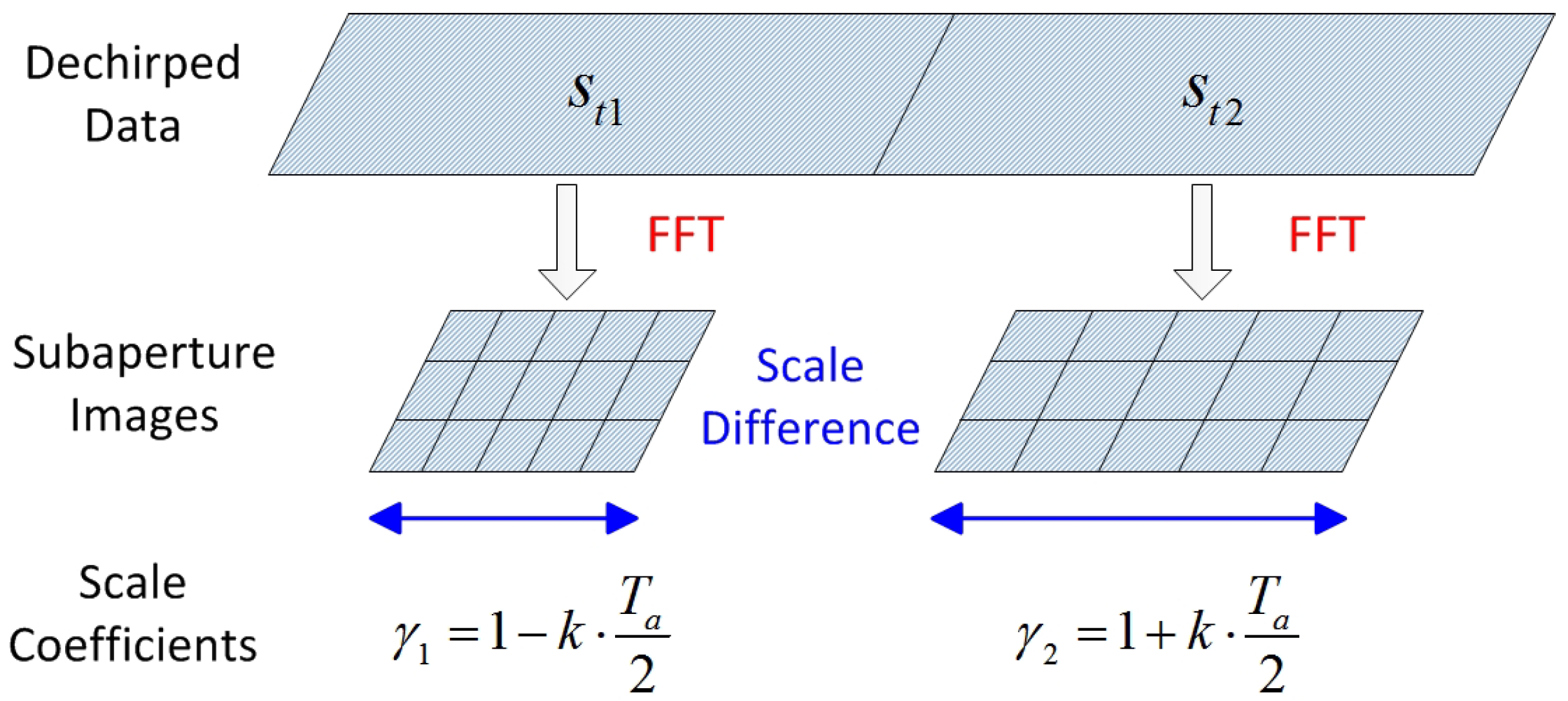
It is clarified in Equations (14) and (15) that scale coefficients of the two subapertures are different. For simplicity, we define them as ${\gamma }_1=\left(1-k·\frac{T_a}{2}\right)$ and ${\gamma }_2=\left(1+k·\frac{T_a}{2}\right)$, respectively. It is obvious that the azimuth scale of subaperture images obtained by FFT changes with respect to the quadratic azimuth-variant coefficient k. Shown in Figure 2, the diagram illustrates the scale difference between subaperture images. By using the image correlation principle to estimate the quadratic phase coefficient, the scaled Fourier transform (SFT) is applied to generate scaled subaperture images. Only when the scale coefficients in SFT coincide with ${\gamma }_1$ and ${\gamma }_2$, the correlation coefficient between the subaperture images will reach a maximum value. To achieve the azimuth-variant coefficient k, we develop a novel solver to the modified maximum cross-correlation optimization in the SFT-based map-drift formation.

2.3. Basic Principle of Proposal

Based on the above analysis of azimuth-variant QPE, the basic principle of the proposed AVMDA is introduced in this subsection. After performing SFT to ${s_t}_1\left(t;\alpha \right)$ and ${s_t}_2\left(t;\alpha \right)$ with coefficients ${\gamma }_1$ and ${\gamma }_2$, we have the subaperture images shown as

$$\begin{array}{ll}{s}_{f1}\left(w;k\right)\hfill & =\underset{-T_a/\phantom{-T_{a}4}4}{\overset{T_a/\phantom{T_{a}4}4}{\int }}{s}_{t1}\left(t;\alpha \right)·exp\left(-j{\gamma }_{1}wt\right)dt\\ & =\underset{-T_a/\phantom{-T_{a}4}4}{\overset{T_a/\phantom{T_{a}4}4}{\int }}\sigma ·exp\left[-j{\gamma }_1\left(w-\alpha \right)t\right]·exp\left[jk\alpha \left(t^2+\frac{T_a^2}{16}\right)\right]dt·exp\left(-j\alpha \frac{T_a}{4}\right)\hfill \end{array}$$

(16)

$$\begin{array}{ll}{s_f}_2\left(w;k\right)\hfill & =\underset{-T_a/\phantom{-T_{a}4}4}{\overset{T_a/\phantom{T_{a}4}4}{\int }}{s}_{t2}\left(t;\alpha \right)·exp\left(-j{\gamma }_{2}wt\right)dt\\ & =\underset{-T_a/\phantom{-T_{a}4}4}{\overset{T_a/\phantom{T_{a}4}4}{\int }}\sigma ·exp\left[-j{\gamma }_2\left(w-\alpha \right)t\right]·exp\left[jk\alpha \left(t^2+\frac{T_a^2}{16}\right)\right]dt·exp\left(j\alpha \frac{T_a}{4}\right).\hfill \end{array}$$

(17)

where, w represents the azimuth spectral function. The explicit expressions of Equations (16) and (17) are given by

$$s_{f1}\left(w;k\right)\approx \sigma ·\mathrm{rect}\left[\frac{{\gamma }_1\left(w-\alpha \right)}{k\alpha T_a}\right]·exp\left[-j\frac{{\gamma }_1^2{\left(w-\alpha \right)}^2}{4k\alpha }\right]·exp\left(-j\alpha \frac{T_a}{4}\right)·exp\left(jk\alpha \frac{T_a^2}{16}\right)$$

(18)

$$s_{f2}\left(w;k\right)\approx \sigma ·\mathrm{rect}\left[\frac{{\gamma }_2\left(w-\alpha \right)}{k\alpha T_a}\right]·exp\left[-j\frac{{\gamma }_2^2{\left(w-\alpha \right)}^2}{4k\alpha }\right]·exp\left(j\alpha \frac{T_a}{4}\right)·exp\left(jk\alpha \frac{T_a^2}{16}\right).$$

(19)

where, $rect\left(·\right)$ represents rectangular window function, and the derivation process is given in Appendix A. It is shown in Equations (18) and (19) that $s_{f1}\left(w;k\right)$ and $s_{f2}\left(w;k\right)$ have similar envelopes along the Doppler frequency w axis, so we assume that

$${\left|s_{f1}\left(w;k\right)\right|}^2\approx {\left|s_{f2}\left(w;k\right)\right|}^2$$

(20)

According to the analysis above, SFT can be performed by using scaling factors ${\gamma }_1$ and ${\gamma }_2$ for a given azimuth-variant Doppler rate $k_{\alpha }$. If we use only the real-scaled coefficients, the subaperture images $s_{f1}\left(w;k\right)$ and $s_{f2}\left(w;k\right)$ have an identical profile. The coherence between ${\left|s_{f1}\left(w;k\right)\right|}^2$ and ${\left|s_{f2}\left(w;k\right)\right|}^2$ can be measured by their cross-correlation coefficient, which is a function of unknown variable k. Then it can be formulated as

$$\mathsf{\Theta }\left(k\right)=\frac{\int {\left|s_{f1}\left(w;k\right)\right|}^2·{\left|s_{f2}\left(w;k\right)\right|}^{2}d\omega }{\sqrt{\int {\left|s_{f1}\left(w;k\right)\right|}^2·{\left|s_{f1}\left(w;k\right)\right|}^{2}d\omega }·\sqrt{\int {\left|s_{f2}\left(w;k\right)\right|}^2·{\left|s_{f2}\left(w;k\right)\right|}^{2}d\omega }}.$$

(21)

One can see that the unknown azimuth-variant Doppler rate $k_{\alpha }$ can be retrieved by maximizing the cross-correlation coefficient function $\mathsf{\Theta }\left(k\right)$. Equation (21) can be simplified as

$$\mathsf{\Theta }\left(k\right)=\int {\left|s_{f1}\left(w;k\right)\right|}^2·{\left|s_{f2}\left(w;k\right)\right|}^{2}d\omega$$

(22)

The estimation of the azimuth-variant coefficient k corresponds to the maximum of the cross-correlation coefficient $\mathsf{\Theta }$.

$$\widehat{k}=\underset{k}{max}\mathsf{\Theta }\left(k\right)$$

(23)

After estimating coefficient $\widehat{k}$, we can efficiently compensate the azimuth-variant phase error by a nonlinear interpolation.

$$t=t^{\prime }-\widehat{k}t{}^{\prime 2}$$

(24)

By substituting Equation (24) into Equation (13), it can be rewritten as

$$s_t\left(t^{\prime },\alpha \right)\approx \sigma ·exp\left(j\alpha t^{\prime }\right)·exp\left[j\left(k-\widehat{k}\right)\alpha t{}^{\prime 2}\right]$$

(25)

So, the compensation precision depends on the precision of estimated $\widehat{k}$.

The basic principle of AVMDA is illustrated in Figure 3. Inheriting the processing strategy of conventional MDA, the disturbed raw data is processed by de-ramping to remove the bulk quadratic phase coefficient first, and then segmented into two subaperture blocks expressed by ${s_t}_1$ and ${s_t}_2$. In the following stages, we aim to estimate the azimuth-variant coefficient k, which is quite different from MDA. In AVMDA, the subaperture data ${s_t}_1$ and ${s_t}_2$ are transformed to obtain a pair of sub-images ${s_f}_1$ and ${s_f}_2$ by CZT, where the scaling factors ${\gamma }_1$ and ${\gamma }_2$ are calculated by the initial azimuth-variant coefficient. We can subsequently calculate the cross-correlation coefficient $\mathsf{\Theta }$ in Equation (22), which is a function of coefficient k. Hence it is feasible to obtain the first-round estimation $\widehat{k}$ by solving the optimization problem in Equation (23). After getting $\widehat{k}$ in the first-round estimation, update azimuth-variant coefficient k by $\widehat{k}$ to compensate the de-ramped data. In this way, the residual azimuth-variant error of de-ramped data gets smaller and smaller after iterations, and the azimuth-variant error in the final data would be removed effectively. Please note that there would be less than three iterations based on our experience. Next we will focus on how to solve the maximum optimization problem in Equation (23).

2.4. Maximum Optimization Solver

To implement an efficient solver to the estimation of k in Equation (23), we give the discrete representation of the derivations in Equations (16) and (17) as follows

$$s_{f1}\left(u\right)=\frac{1}{M}\sum _{m=0}^{M-1}exp\left[-j2\pi \frac{um}{M}\left(1-k\Delta T\right)\right]·s_{t1}\left(m\right)$$

(26)

$$s_{f2}\left(u\right)=\frac{1}{M}\sum _{m=0}^{M-1}exp\left[-j2\pi \frac{um}{M}\left(1+k\Delta T\right)\right]·s_{t2}\left(m\right)$$

(27)

where $\Delta T=T_a/\phantom{T_{a}2}2$, M denotes the discrete Fourier transform (DFT) length, m denotes the discrete time domain axis, u denotes the discrete frequency domain spectrum. According to Equation (22), the cross-correlation coefficient of the two subaperture images can be calculated by

$$\mathsf{\Theta }\left(k\right)=\frac{1}{M}\sum _{u=0}^{M-1}{\left|s_{f1}\left(u\right)\right|}^2·{\left|s_{f2}\left(u\right)\right|}^2=\frac{1}{M}\sum _{u=0}^{M-1}\left[s_{f1}\left(u\right)·s_{{}_{f1}}^{*}\left(u\right)\right]·\left[s_{f2}\left(u\right)·s_{{}_{f2}}^{*}\left(u\right)\right]$$

(28)

In practice, the one-dimensional searching method is an effective strategy to solve Equation (23). This method approximates the extreme point of objective function step by step, so the searching step is an important factor in determining the operational efficiency and reliability directly. Newton optimization algorithm is one of the most widely used one-dimensional searching methods. As the objective function is continuous and twice differentiable, according to the principle of matrix calculation in Zhang (2011) [48], the first-order and second-order partial derivatives of the objective function are calculated to determine the searching step, which are shown as follows

$$\frac{\partial \mathsf{\Theta }\left(k\right)}{\partial k}=\frac{1}{M}\sum _{u=0}^{M-1}{\left|s_{f1}\left(u\right)\right|}^2·\frac{\partial \left[s_{f2}\left(u\right)·s_{{}_{f2}}^{*}\left(u\right)\right]}{\partial k}+{\left|s_{f2}\left(u\right)\right|}^2·\frac{\partial \left[s_{f1}\left(u\right)·s_{{}_{f1}}^{*}\left(u\right)\right]}{\partial k}$$

(29)

$$\frac{{\partial }^2\mathsf{\Theta }\left(k\right)}{{\partial }^{2}k}=\frac{1}{M}\sum _{u=0}^{M-1}\left[\begin{array}{c}2\frac{\partial \left[s_{f1}\left(u\right)·s_{{}_{f1}}^{*}\left(u\right)\right]}{\partial k}·\frac{\partial \left[s_{f2}\left(u\right)·s_{{}_{f2}}^{*}\left(u\right)\right]}{\partial k}+\hfill \\ {\left|s_{f1}\left(u\right)\right|}^2·\frac{{\partial }^2\left[s_{f2}\left(u\right)·s_{{}_{f2}}^{*}\left(u\right)\right]}{{\partial }^{2}k}+{\left|s_{f2}\left(u\right)\right|}^2·\frac{{\partial }^2\left[s_{f1}\left(u\right)·s_{{}_{f1}}^{*}\left(u\right)\right]}{{\partial }^{2}k}\hfill \end{array}\right]$$

(30)

where the first-order partial derivative terms in Equations (29) and (30) are calculated by

$$\frac{\partial \left[s_{f1}\left(u\right)·s_{{}_{f1}}^{*}\left(u\right)\right]}{\partial k}=2·\mathrm{Re}\left[s_{{}_{f1}}^{*}\left(u\right)\frac{\partial s_{f1}\left(u\right)}{\partial k}\right]$$

(31)

$$\frac{\partial \left[s_{f2}\left(u\right)·s_{{}_{f2}}^{*}\left(u\right)\right]}{\partial k}=2·\mathrm{Re}\left[s_{{}_{f2}}^{*}\left(u\right)\frac{\partial s_{f2}\left(u\right)}{\partial k}\right]$$

(32)

The second-order partial derivatives in Equation (30) are calculated by

$$\frac{{\partial }^2\left[s_{f1}\left(u\right)·s_{{}_{f1}}^{*}\left(u\right)\right]}{{\partial }^{2}k}=2·\mathrm{Re}\left[\frac{\partial s_{{}_{f1}}^{*}\left(u\right)}{\partial k}·\frac{\partial s_{f1}\left(u\right)}{\partial k}+s_{{}_{f1}}^{*}\left(u\right)\frac{{\partial }^2{s}_{f1}\left(u\right)}{{\partial }^{2}k}\right]$$

(33)

$$\frac{{\partial }^2\left[s_{f2}\left(u\right)·s_{{}_{f2}}^{*}\left(u\right)\right]}{{\partial }^{2}k}=2·\mathrm{Re}\left[\frac{\partial s_{{}_{f2}}^{*}\left(u\right)}{\partial k}·\frac{\partial s_{f2}\left(u\right)}{\partial k}+s_{{}_{f2}}^{*}\left(u\right)\frac{{\partial }^2{s}_{f2}\left(u\right)}{{\partial }^{2}k}\right]$$

(34)

According to the sub-image discrete representations in Equations (26) and (27), the first-order partial derivatives in Equations (33) and (34) are calculated by

$$\frac{\partial s_{f1}\left(u\right)}{\partial k}=\frac{1}{M}\sum _{m=0}^{M-1}j2\pi \frac{um}{M}\Delta T·exp\left[-j2\pi \frac{um}{M}\left(1-k\Delta T\right)\right]·s_{t1}\left(m\right)$$

(35)

$$\frac{\partial s_{f2}\left(u\right)}{\partial k}=-\frac{1}{M}\sum _{m=0}^{M-1}j2\pi \frac{um}{M}\Delta T·exp\left[-j2\pi \frac{um}{M}\left(1+k\Delta T\right)\right]·s_{t2}\left(m\right)$$

(36)

The second-order partial derivatives in Equations (33) and (34) are calculated by

$$\frac{{\partial }^2{s}_{f1}\left(u\right)}{{\partial }^{2}k}=\frac{1}{M}\sum _{m=0}^{M-1}{\left(j2\pi \frac{um}{M}\Delta T\right)}^2·exp\left[-j2\pi \frac{um}{M}\left(1-k\Delta T\right)\right]·s_{t1}\left(m\right)$$

(37)

$$\frac{{\partial }^2{s}_{f2}\left(u\right)}{{\partial }^{2}k}=\frac{1}{M}\sum _{m=0}^{M-1}{\left(-j2\pi \frac{um}{M}\Delta T\right)}^2·exp\left[-j2\pi \frac{um}{M}\left(1+k\Delta T\right)\right]·s_{t2}\left(m\right)$$

(38)

According to Newton optimization principle, the searching step $\Delta d$ is then calculated by

$$\Delta d=\frac{\partial \mathsf{\Theta }\left(k\right)}{\partial k}/\left|\frac{{\partial }^2\mathsf{\Theta }\left(k\right)}{{\partial }^{2}k}\right|$$

(39)

where $\left|·\right|$ denotes the absolute value operation, and $\Delta d$ determines the search direction.

From the above analysis, we know that Newton optimization algorithm can approach the extreme point gradually by iterative operation. However, it remains a significant problem in practical applications that we cannot make sure the object function declining after each searching step, which would cause convergence speed decreasing. Therefore, we need to optimize the searching step by setting a condition to ensure the decline of the object function. Armijo step optimization [49] is an effective strategy to select an appropriate searching step. According to the purpose, set the termination condition as follows

$$\mathsf{\Theta }\left(k+\Delta d^{\left(n\right)}\right)>\mathsf{\Theta }\left(k\right)+{\tau }^{n-1}\Delta d^{\left(0\right)}·\partial \mathsf{\Theta }/\partial k$$

(40)

or

$$\mathsf{\Theta }\left(k+\Delta d^{\left(n\right)}\right)>\mathsf{\Theta }\left(k\right)$$

(41)

where $\tau \in \left(0,1\right)$ is a constant reduction factor, $\Delta d^{\left(0\right)}$ denotes the initial searching step calculated by Equation (39) and its sign represents the searching direction, and n denotes the judgment times. As for the nth judgment, searching step $\Delta d^{\left(n\right)}$ becomes ${\tau }^{n-1}·\Delta d^{\left(0\right)}$. The judgment will continue until reaching the termination condition.

Besides, since the computational burden of initial searching step $\Delta d^{\left(0\right)}$ is considerable, we need to calculate the first-order and second-order partial derivatives in each iteration, which is computationally expensive and unacceptable for real-time data processing. By considering the termination condition which is set to ensure the convergence property, it is possible to achieve a balance between the initial searching step accuracy and processing efficiency. According to the principle of BFGS (Broyden, Fletcher, Goldfard and Shanno) [50] algorithm, the second-order partial derivative matrix (Hessian matrix) can be calculated approximately by an updated formula as follows.

$$\frac{{\partial }^2\mathsf{\Theta }{\left(k\right)}^{\left(n+1\right)}}{{\partial }^{2}k}=\frac{{\partial }^2\mathsf{\Theta }{\left(k\right)}^{\left(n\right)}}{{\partial }^{2}k}+\frac{\Delta \frac{\partial \mathsf{\Theta }{\left(k\right)}^{\left(n\right)}}{\partial k}·{\left[\Delta \frac{\partial \mathsf{\Theta }{\left(k\right)}^{\left(n\right)}}{\partial k}\right]}^T}{{\left[\Delta \frac{\partial \mathsf{\Theta }{\left(k\right)}^{\left(n\right)}}{\partial k}\right]}^T·\Delta {\widehat{k}}^{\left(n\right)}}-\frac{\frac{{\partial }^2\mathsf{\Theta }{\left(k\right)}^{\left(n\right)}}{{\partial }^{2}k}·\Delta {\widehat{k}}^{\left(n\right)}·{\left[\Delta {\widehat{k}}^{\left(n\right)}\right]}^T·\frac{{\partial }^2\mathsf{\Theta }{\left(k\right)}^{\left(n\right)}}{{\partial }^{2}k}}{{\left[\Delta {\widehat{k}}^{\left(n\right)}\right]}^T·\frac{{\partial }^2\mathsf{\Theta }{\left(k\right)}^{\left(n\right)}}{{\partial }^{2}k}·\Delta {\widehat{k}}^{\left(n\right)}}$$

(42)

where the superscript denotes the iteration times, and $\Delta$ demotes the subtraction operation with the last iteration result. For the problem of this paper, cross-correlation coefficient $\mathsf{\Theta }$ is a scalar quantity, so Equation (42) is degenerated to a one-dimensional expression.

$$\frac{{\partial }^2\mathsf{\Theta }{\left(k\right)}^{\left(n+1\right)}}{{\partial }^{2}k}=\Delta \frac{\partial \mathsf{\Theta }{\left(k\right)}^{\left(n\right)}}{\partial k}/\Delta {\widehat{k}}^{\left(n\right)}$$

(43)

The flowchart of the proposed maximum optimization problem solver is provided in Figure 4, which is implemented by a loop iteration. At the beginning of the procedure, an initial coefficient k is determined. By using the processing strategy shown in Figure 3, two sub-images will be obtained in order to calculate the first-order and second-order partial derivatives of objective function $\partial \mathsf{\Theta }\left(k\right)/\phantom{\partial \mathsf{\Theta }\left(k\right)\partial k}\partial k$ and ${\partial }^2\mathsf{\Theta }\left(k\right)/{\partial }^{2}k$ by Equations (29) and (30). Searching step $\Delta d$ is then calculated by Equation (39) based on Newton optimization principle.

To improve the convergence performance of the quadratic Newton solver, searching step $\Delta d$ needs to be optimized. Armijo step optimization method is introduced to set conditions for the searching step so that the drooping characteristic in each iteration will be ensured. We calculate the cross-correlation coefficient $\mathsf{\Theta }$ with the current searching step, and then judge whether it satisfies the Armijo condition. If not, update the searching step $\Delta d$ by multiplying a constant coefficient. This cycle judgment will not stop until the Armijo termination condition is met. After finding a proper step, we can update the initial coefficient k and enable a new loop iteration. The second-order derivative ${\partial }^2\mathsf{\Theta }\left(k\right)/\phantom{{\partial }^2\mathsf{\Theta }\left(k\right){\partial }^{2}k}{\partial }^{2}k$ can also be efficiently calculated by BFGS in approximation during each iteration. The estimated azimuth-variant coefficient k will barely shift after several iterations, and then the loop can be terminated.

2.5. Procedure of Proposal

As a summary of this section, a concise procedure of AVMDA is provided in

Table 1. Procedure of proposed AVMDA.

Algorithm: The proposed AVMDA

Input Data

De-ramping

Initializek

Repeat

Calculation$\mathsf{\Theta }\left(k\right)=\frac{1}{M}{\displaystyle \sum _{u=0}^{M-1}}\left[s_{f1}\left(u\right)·s_{{}_{f1}}^{*}\left(u\right)\right]·\left[s_{f2}\left(u\right)·s_{{}_{f2}}^{*}\left(u\right)\right]$

Optimization$\widehat{k}=max\mathsf{\Theta }\left(k\right)$

Updatek

Until Convergence

Outputk

. The process consists of the following steps:

(a) Input Data. After conventional processing such as range pulse compression, MOCO and Range Cell Migration Correction (RCMC), the data disturbed with azimuth-variant phase error is input in this step.

(b) De-ramping. By now, the data is ready for the application of AVMDA autofocus. De-ramping is an essential process to remove the quadratic term in Equation (7), where the de-ramping reference function for sample at coordinate r is expressed as

$$h_{ref}\left(t,r\right)=exp\left(j{K}_{rc}\frac{v^2{cos}^2\phi }{2r}·t^2\right)$$

(44)

Multiplying Equation (44) with $h_{ref}\left(t,r\right)$ on both sides of Equation (7) and neglecting the constant phase, azimuth-invariant phase, and high-order phase terms, we have

$$s_t\left(X,r,x\right)\approx \sigma ·exp\left(j\frac{K_{rc}v·x}{r}·t\right)·exp\left[-j\Delta k\left(r,\alpha \right)t^2\right]$$

(45)

Please note that Equation (45) is similar to the model defined in Equation (11). In this case, we have

$$\alpha =\frac{K_{rc}v}{r}·x$$

(46)

(c) Initialize. The linear coefficient k of azimuth-variant phase error can be initialized to $k=0$.

(d) Cyclic iterative estimation. The azimuth-variant coefficient $\widehat{k}$ would be successively achieved by a finite iterative manner. In the steps of each iteration, the linear coefficient k obtained from the previous step is used to calculate the correlation coefficient in Equation (22). Then, use the optimization method given in Figure 4 to solve and update coefficient k until the convergence.

(e) Output. The convergent linear coefficient k is output, and then the azimuth-variant phase error is compensated easily by the interpolation process in Equations (24) and (25).

However, it should be noted that in real UAV SAR imagery circumstances, MOCO with low-precision IMU system would leave significant residual two-dimensional spatial-variant phase errors. In this case, it is necessary to develop an effective strategy to ensure the focusing performance of imagery.

3. Extending to Two-Dimensional Spatial-Variant Map-Drift Algorithm

3.1. Procedure of Proposal

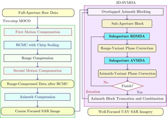
In this section, we discuss how to embed AVMDA into the UAV SAR imaging procedure and simultaneously achieve two-dimensional spatial-variant autofocus in both range and azimuth directions. There are some novel MOCO strategies that can be applied to UAV SAR MOCO. However, it is more important for UAV SAR imagery to deeply use available IMU data and reduce most motion errors with coarse MOCO. After that, the residual phase error contains mixed components, including variant and invariant components in range and azimuth directions, which are expected to be corrected by an integrated autofocus technique. The block diagram of UAV SAR imaging by using an integrated MOCO with RDMDA and AVMDA is shown in Figure 5. In the procedure above, the RDMDA and AVMDA approaches are concatenate in the chirp-scaling processing with the “two-step”MOCO strategy. Then the autofocus MOCO stage is named by 2D-SVMDA in this paper. According to the block diagram, the UAV SAR processing algorithm has the following key steps:

(a) Coarse MOCO. In the beginning stage, a coarse MOCO is processed with assistant navigation measurements such as airborne INS, so that most of motion errors could be compensated. The most common coarse MOCO algorithm is "two-step" MOCO, which is divided into a bulk MOCO step and a range-dependent MOCO step. However, due to the inadequate precision of INS equipped on UAV, we need the autofocus algorithm to compensate the residual phase errors.

(b) RCMC. This step is known as the conventional processing of SAR imaging. According to the block diagram in Figure 5, RCMC is implemented with chirp-scaling algorithm (CSA) in the range-Doppler domain, and the range compression is achieved simultaneously. Please note that other RCMC algorithms, such as range-Doppler algorithm (RDA) and Omega-k algorithm, are also suitable for UAV SAR imagery.

(c) Azimuth blocking. For practical UAV SAR imaging, azimuth blocking operation is necessary before using 2D-SVMDA. In contrast to conventional azimuth blocking strategies, we do not need to segment data into many small blocks to make sure the invariance of phase error is within each processing block. The azimuth block size can be enlarged and the azimuth-variant phase error in each sub-block would be estimated. This azimuth blocking enhances the efficiency and robustness of data processing.

(d) RDMDA. During real UAV SAR imaging with wide swath, the range-dependence of motion error is usually severe. In addition, due to the limited INS precision, the coarse MOCO step is not able to compensate the range-variant motion error precisely. For this reason, RDMDA is introduced to estimate the residual range-variant phase error. Suppose $\Delta k\left(r,\alpha \right)$ in Equation (45) is expressed by

$$\Delta k\left(r,x\right)=a+b·r+k·\alpha$$

(47)

where a is the range- and azimuth-invariant QPE coefficient, b is the range-variant QPE coefficient, and k is the azimuth-variant QPE coefficient. By applying RDMDA to the de-ramped data, we can estimate both range-invariant and variant QPE coefficients $\widehat{a}$ and $\widehat{b}$.

(e) AVMDA. Based on the introduction to AVMDA principle in Section 2, we mainly focus on the azimuth-variant QPE coefficient k estimation in this step. After estimating the coefficient $\widehat{k}$, according to Equations (45) and (46), we can compensate the azimuth-variant phase error by a nonlinear interpolation shown in Equation (24).

In the proposed 2D-SVMDA strategy, it should be emphasized that an iteration of estimation and compensation loop is required to remove the residual range- and azimuth-variant phase for full-aperture processing. When the processing data is polluted by strong noise or there are not adequate prominent targets in the scene, it needs to non-coherently sum up the cross-correlation functions of some prominent range bins to enhance the accuracy of QPE linear coefficient estimation. Finally, after sequentially truncating and combining each azimuth sub-block, a well-focused UAV SAR imagery would be obtained.

3.2. Application Hypothesis and Limitation

In practical applications, the method proposed in this paper needs to follow two assumptions.

(a) The envelope error component can be corrected by using inertial navigation information and “two-step” MOCO method. The proposed algorithm only aims at the estimation and compensation for phase errors.

(b) The non-spatial variation error is the main component of the data, and the residual spatial-variant error is a relatively minor component. When the spatial-variant error increases, the number of iterations of 2D-SVMDA in Figure 5 will increase accordingly, which will affect the efficiency of the algorithm.

In general, the assumptions above are satisfiable. Under these assumptions, the residual spatial-variant motion error should not exceed one range bin. Otherwise, it will affect the calculation accuracy of sub-image correlation coefficient. Assume a range bin is $\Delta r$, the scene width in azimuth direction is $L_x$, and the scene width in range direction is $L_r$. Then the limitation of linear coefficient of azimuth-variant phase error $k_{max}$ is

$$k_{max}=\frac{4\pi \Delta r}{\lambda L_a}$$

(48)

Similarly, the limitation of linear coefficient of azimuth-variant phase error $b_{max}$ is

$$b_{max}=\frac{4\pi \Delta r}{\lambda L_r}$$

(49)

3.3. Computational Burden Analysis

In this subsection, we theoretically analyze the computational burden of the proposed algorithm by computing the floating-point operations (FLOPs) caused by FFT/IFFT operation. Assume the azimuth length of data is N, and M range bins with strong reflection are selected from the data for error parameter estimation. According to the description in [32], there are 4M times N/2-point FFT/IFFT in each iteration step of RDMDA. For the AVMDA proposed in this paper, there are 2M times N/2-point CZT operations in each iteration step, and each CZT operation contains 3 times FFT/IFFT. One N-point FFT/IFFT operation contains $5N{log}_2\left(N\right)$ FLOPs, so for three iterations, the computational burden of 2D-SVMDA is given by

$$\begin{array}{cc}C\hfill & =3\times \left[4M·\frac{5}{2}N{log}_2\left(\frac{N}{2}\right)+6M·\frac{5}{2}N{log}_2\left(\frac{N}{2}\right)\right]\\ & =75M·N·{log}_2\left(\frac{N}{2}\right)\hfill \end{array}$$

(50)

4. Simulated and Real Measured Data Experiments

To validate the effectiveness of the proposed AVMDA and 2D-SVMDA autofocus strategies, four sets of experiments are performed with simulated and real measured X-band and Ka-band SAR data in this section. In the simulation experiments, we artificially introduce azimuth-variant and range-variant QPE into the simulated data. The introduced phase errors vary linearly in range and azimuth directions, respectively, where the azimuth-variant QPE linear coefficient is indicated as k, and the range-variant QPE linear coefficient is indicated as b.

The measured data are provided by the National Lab of Radar Signal Processing and Collaborative Innovation Center of Information Sensing and Understanding of Xidian University. There is not additional phase error artificially added into the measured data. Defocusing on imaging is mainly caused by residual range and azimuth-variant phase errors after conventional “two-step” MOCO. The imaging method used in experiments is based on RDA. The computer platform is Windows7 (Microsoft Corporation, Redmond, Washington, USA) 64-bit operating system, [email protected] GHz CPU, 32 GB memory and MATLAB (MathWorks Corporation, Natick, Massachusetts, USA) Version R2014a.

4.1. X-Band Simulation Experiments

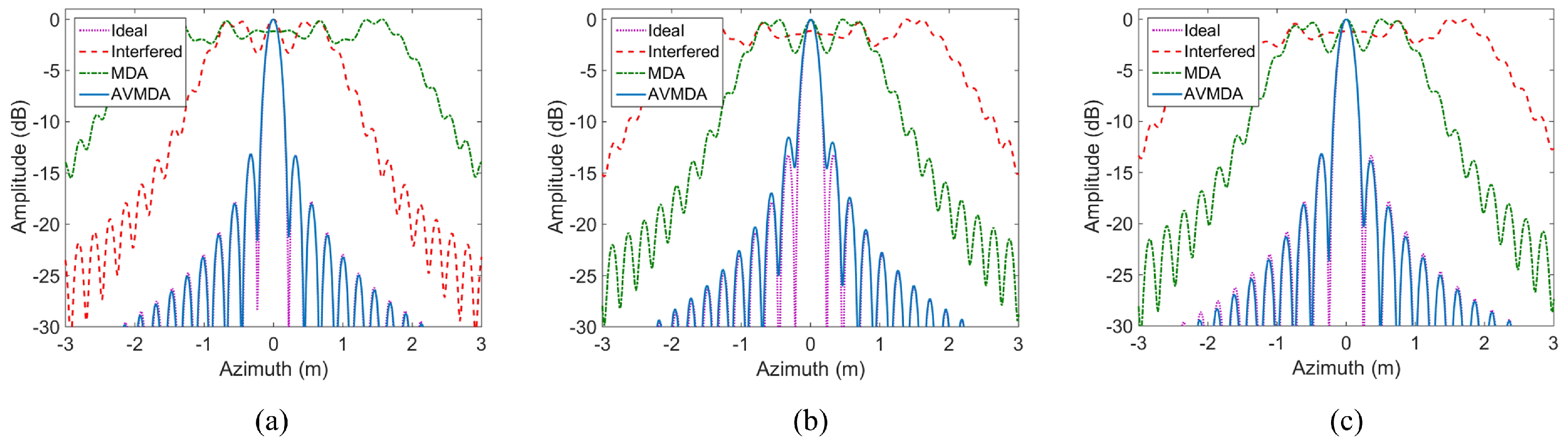
The main simulation parameters of the experiment on X-band are shown in

Table 2. X-Band simulation parameters.

Carrier frequency	9 GHz
Pulse repetition frequency	2000 Hz
Velocity	100 m/s
Pulse width	2 $\mathsf{\mu }$s
Center closest slant range	4.5 km
Squint angle	0 degree
Grazing angle	45 degrees
Range resolution	1 m
Azimuth resolution	1 m

. A two-dimensional dot matrix is designed to simulate a scene with strong scatters. The size of simulated data is 8192 × 8192 (azimuth × range). In this subsection, the purpose of the first simulation is to verify the performance of AVMDA. We presuppose azimuth-variant QPE linear coefficient $k=0.1$, and the data is processed with conventional MDA and AVMDA for comparison. Dot matrix imaging results and their magnified sub-scenes are shown in Figure 6, in which (a) to (d) are ideal point image, azimuth-variant error interfered image, conventional MDA processed image, and AVMDA processed image, respectively. Three points named “A”, “B” and “C” are highlighted by yellow circles, and we analyze their azimuth impulse response functions as shown in Figure 7. To quantitatively evaluate the focused improvement of the proposed AVMDA compared with the other algorithms, three quantitative metrics are introduced to measure the point impulse response functions, which are peak side-lobe ratio (PSLR), integrated side-lobe ratio (ISLR), and impulse response width (IRW). The results are shown in

Table 3. Statistical focus comparison of ideal, azimuth-variant error interfered, MDA processed, and AVMDA processed simulated point targets.

Approach	Point A			Point B			Point C
	PSLR (dB)	ISLR (dB)	IRW (m)	PSLR (dB)	ISLR (dB)	IRW (m)	PSLR (dB)	ISLR (dB)	IRW (m)
Ideal	−13.1689	−10.7262	1.0750	−12.9831	−10.6136	0.9100	−13.2438	−10.6689	1.0860
Interfered	−5.2130	−4.3508	2.3875	−4.8707	−3.5794	2.5200	−4.9914	−3.7235	2.4765
MDA	−9.6775	−7.3409	1.1625	−8.0726	−5.9907	1.0415	−2.1579	−0.1272	2.8905
AVMDA	−12.8934	−10.4524	1.0875	−12.7604	−10.2128	0.9100	−13.1371	−10.5467	1.0940

.

It can be seen that the azimuth-variant phase error severely defocuses the points. Due to the weakness in dealing with the azimuth-variant phase error, conventional MDA is not able to refocus all the defocused points. In contrast, by precisely estimating the linear azimuth-variant QPE factor, the refocusing performances of points in AVMDA are very close to the ideally focused ones.

To verify the performance of 2D-SVMDA, a second experiment is designed by simultaneously introducing range- and azimuth-variant QPE linear coefficients with $b=0.003$ and $k=0.1$. By considering the impact of range- and azimuth-variant phase errors, it is difficult to remove all the phase errors by conventional MDA or RDMDA. To compare the compensation performance of different autofocus methods, point target simulation results and magnified sub-scenes are shown in Figure 8, in which (a) to (d) are range- and azimuth-variant error interfered image, conventional MDA processed image, RDMDA processed image, and 2D-SVMDA processed image, respectively. Azimuth impulse response functions and corresponding quantitative results of Points A, B, and C (highlighted in Figure 8) are shown in Figure 9 and

Table 4. Statistical focus comparison of ideal, 2D spatial-variant error interfered, MDA processed, RDMDA processed, and 2D-SVMDA processed simulated point targets.

Approach	Point A			Point B			Point C
	PSLR (dB)	ISLR (dB)	IRW (m)	PSLR (dB)	ISLR (dB)	IRW (m)	PSLR (dB)	ISLR (dB)	IRW (m)
Ideal	−13.0574	−10.7079	1.1025	−13.3105	−10.7299	1.0915	−13.2438	−10.6689	1.0860
Interfered	−0.0977	2.6361	4.8485	−5.2782	−3.8570	2.4415	−0.1151	3.8709	5.9295
MDA	−0.1083	4.4114	6.1760	−1.5718	0.8941	3.0265	−0.0435	3.1508	4.6795
RDMDA	−2.4122	−0.6264	2.9135	−5.1747	−3.7834	2.4525	−2.2886	−0.2107	2.8670
2D-SVMDA	−12.7364	−10.3042	1.1140	−13.1904	−10.6469	1.0915	−13.1740	−10.2391	1.0940

.

It can be seen that the imaging result is blurred due to the range- and azimuth-variant phase errors. Serious defocusing remains in conventional MDA processed and RDMDA processed results, only the proposed 2D-SVMDA can refocus the whole scene in this situation. With the iterative application of RDMDA and AVMDA, the induced range- and azimuth-variant phase errors decrease gradually so that the performance of autofocus result processed by 2D-SVMDA is highly close to the ideal one.

4.2. Ka-Band Simulation Experiments

Similar to the X-band simulation experiments, Ka-band simulation experiments are designed to verify the performance of processed AVMDA and 2D-SVMDA working at high frequencies, such as the millimeter wave band. The main simulation parameters of experiments on Ka-band are shown in

Table 5. Ka-Band simulation parameters.

Carrier frequency	35 GHz
Pulse repetition frequency	2000 Hz
Velocity	100 m/s
Pulse width	2 $\mathsf{\mu }$s
Center closest slant range	4.5 km
Squint angle	0 degree
Grazing angle	45 degrees
Range resolution	0.3 m
Azimuth resolution	0.3 m

. The size of simulated data is 8192 × 8192 (azimuth × range). In the first experiment, azimuth-variant QPE linear coefficient $k=0.1$ is introduced into the simulated data. Dot matrix imaging results and their magnified sub-scenes are shown in Figure 10, in which (a) to (d) are ideal point image, azimuth-variant error interfered image, conventional MDA processed image, and AVMDA processed image, respectively. Azimuth impulse response functions and corresponding quantitative results of Points A, B, and C (highlighted in Figure 10) are shown in Figure 11 and

Table 6. Statistical focus comparison of ideal, azimuth-variant error interfered, MDA processed, and AVMDA processed simulated point targets.

Approach	Point A			Point B			Point C
	PSLR (dB)	ISLR (dB)	IRW (m)	PSLR (dB)	ISLR (dB)	IRW (m)	PSLR (dB)	ISLR (dB)	IRW (m)
Ideal	−13.2062	−10.7561	0.2970	−13.2443	−10.6704	0.2970	−13.2771	−10.8155	0.3125
Interfered	−0.1938	5.2196	2.1250	−0.0778	9.6198	4.4530	−0.0490	9.6698	4.7815
MDA	−0.0409	10.0784	4.3750	−0.0470	5.9256	2.1720	−0.0320	6.3589	2.3280
AVMDA	−13.1125	−10.7103	0.2970	−11.4852	−9.4408	0.3125	−13.1375	−11.0655	0.3125

. It is demonstrated that AVMDA performs well when dealing with azimuth-variant QPE for high frequency band and high-resolution SAR imaging.

The second experiment is designed to verify the performance of the proposed 2D-SVMDA working at Ka-band. The presupposed range- and azimuth-variant QPE linear coefficients are $b=0.003$ and $k=0.1$, respectively. The point target simulation results and magnified sub-scenes are shown in Figure 12, in which (a) to (d) are range- and azimuth-variant error interfered image, conventional MDA processed image, RDMDA processed image, and 2D-SVMDA processed image, respectively. Azimuth impulse response functions and corresponding quantitative results of Point A, B, and C (highlighted in Figure 12) are shown in Figure 13 and

Table 7. Statistical focus comparison of ideal, 2D spatial-variant error interfered, MDA processed, RDMDA processed and 2D-SVMDA processed simulated point targets

Approach	Point A			Point B			Point C
	PSLR (dB)	ISLR (dB)	IRW (m)	PSLR (dB)	ISLR (dB)	IRW (m)	PSLR (dB)	ISLR (dB)	IRW (m)
Ideal	−13.2520	−10.7007	0.2970	−13.2360	−10.6795	0.3125	−13.3276	−10.7962	0.3125
Interfered	−0.0153	10.1942	5.3440	−5.3242	−7.2027	0.6720	−0.2429	9.8641	5.0470
MDA	−0.0222	10.1312	7.6565	−0.0440	7.7950	3.1405	−0.1581	3.9971	2.6565
RDMDA	−0.0114	5.0664	2.1095	−0.0459	3.4940	1.7815	−0.1635	5.2516	2.2345
2D-SVMDA	−13.0390	−10.5583	0.2970	−12.8603	−10.5048	0.3125	−12.7429	−10.5057	0.3280

. As can be seen, 2D-SVMDA performs the best when dealing with range- and azimuth-variant QPE, because the two-dimensional space-variant phase errors can be simultaneously compensated by the proposed 2D-SVMDA.

4.3. X-Band Real Measured Data Experiments

In this subsection, an X-band real measured UAV SAR experiment is designed. The raw data is collected by an experimental UAV SAR system. The main SAR system parameters are listed in

Table 8. X-Band SAR system parameters.

Carrier frequency	9 GHz
Pulse repetition frequency	500 Hz
Velocity	60 m/s
Height	3000 m
Center closest slant range	10 km
Squint angle	0 degree
Range resolution	0.75 m
Azimuth resolution	0.75 m

with 16,384-point azimuth samples. The radar platform is equipped with a medium-accuracy IMU and a GPS system whose output rate is 5 Hz. The altitude control is at an accuracy of 3 m, and the IMU provides trajectory information at the velocity accuracy of 0.1 m/s in three dimensions. Due to the inaccuracy of INS, after a standard “two-step” MOCO with the INS data, residual range- and azimuth-variant phase errors remain so that we need an autofocus algorithm to generate high quality images.

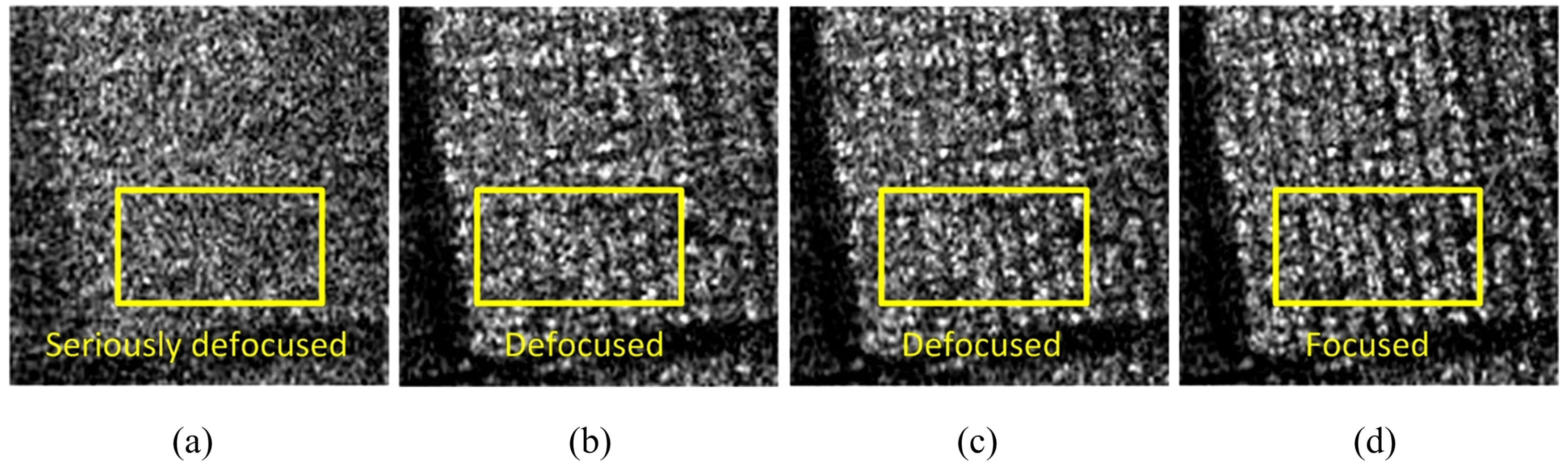
An image block with the size of 900 × 1800 (azimuth × range) is picked and processed by different autofocus strategies for comparison. This image block contains three groups of calibration points at the right side of scene. The refocused results are shown in Figure 14, in which (a) to (d) are processed with INS-only-based “two-step” MOCO, conventional MDA, RDMDA, and the proposed 2D-SVMDA. Apparently, the image generated by the INS-only MOCO is seriously blurred and distorted in geometry due to the lack of accurate motion measurements. To compare the performance of different algorithms more clearly, two sub-scenes with obvious characteristics are magnified, which are shown in Figure 15 and Figure 16, respectively. In Figure 15, there is a man-made structure in this sub-scene. It is obvious that the image is seriously defocused with INS-only MOCO, and partially defocused with conventional MDA and RDMDA, while with 2D-SVMDA autofocus processing, the surface features are distinguishable and focused. Figure 16 shows three groups of calibration points, and it is easier to compare the performance of different autofocus algorithms. We can distinguish all the calibration points only in 2D-SVMDA autofocus processed image. To make a further comparison, two calibration points in Figure 16 are sampled to analyze the azimuth pulse response function, which are shown in Figure 17. The quantitative results of Point A and Point B are listed in

Table 9. Statistical focus comparison of Non-autofocus, MDA processed, RDMDA processed and 2D-SVMDA processed Point A and Point B.

Approach	Point A			Point B
	PSLR (dB)	ISLR (dB)	IRW (m)	PSLR (dB)	ISLR (dB)	IRW (m)
Non-autofocus	−0.2483	7.6671	7.9350	−0.1933	7.1009	10.5360
MDA	−2.9363	−1.2629	3.4040	−3.5827	−5.1773	3.1650
RDMDA	−4.6002	−3.7517	1.4730	−5.2905	−6.6090	1.9310
2D-SVMDA	−11.8845	−8.4139	0.7165	−9.9091	−7.8774	0.7760

. By precisely compensating the range- and azimuth-variant phase errors, the observed points could be focused with high precision. Finally, it can be concluded that the proposed 2D-SVMDA autofocus approach has robust performance for the X-band UAV SAR imagery.

4.4. Ka-Band Real Measured Data Experiments

In this subsection, we also provide a Ka-band measured SAR experiment, in which the raw data is collected by a trial airborne SAR system. The main SAR system parameters are shown in

Table 10. Ka-Band SAR system parameters.

Carrier frequency	35 GHz
Pulse repetition frequency	1000 Hz
Velocity	70 m/s
Height	3000 m
Center closest slant range	4.5 km
Squint angle	0 degree
Range resolution	0.15 m
Azimuth resolution	0.15 m

with 16,384-point azimuth samples. Because the weather condition during the flight test is unsatisfactory, the measured data is burred with heavy motion errors. After conventional “two-step” MOCO, the residual azimuth-variant motion error is still so large that we need to remove it for accurate imaging. In this paper, the main purpose is to remove the residual range- and azimuth-variant motion errors by the proposed 2D-SVMDA autofocus approach, so we conduct the experiments with two-step INS-only MOCO, conventional MDA, RDMDA, and the proposed 2D-SVMDA.

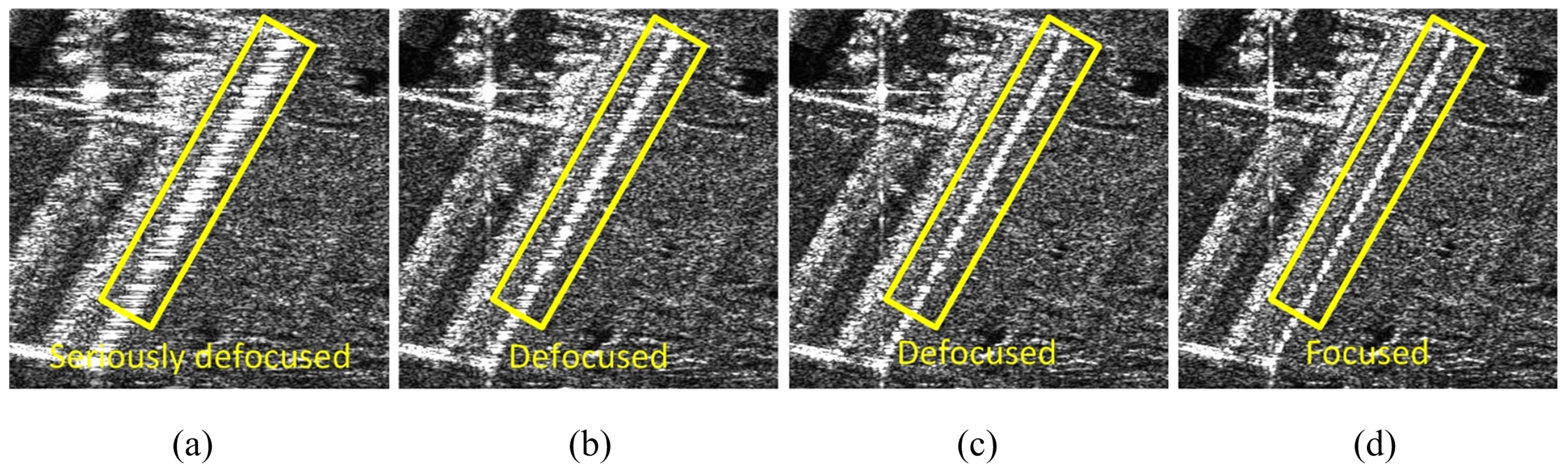
An image block with the size of 2048 × 4096 (azimuth × range) is picked, which contains manufactured constructions in this scene. The comparison results processed by different autofocus strategies are shown in Figure 18. Two sub-scenes containing single construction and point-like targets are highlighted by yellow rectangles in Figure 19, and they are magnified to compare the performance of different autofocus algorithms more clearly in Figure 20. By considering the severe motion deviations, the image processed by “two-step” INS-only MOCO is seriously blurred because of the residual range- and azimuth-variant phase errors, while conventional MDA and RDMDA partly refocus the image. As a contrast, assuming the residual range- and azimuth-variant phase errors is a linear function with respect to the slow time, we obtain a well-focused image by applying the proposed 2D-SVMDA. Furthermore, in Figure 21, we compare the azimuth pulse response functions of the two point-like targets marked in Figure 20. Statistical indicators including PSLR, ISLR, and IRW are listed in

Table 11. Statistical focus comparison of Non-autofocus, MDA processed, RDMDA processed, and 2D-SVMDA processed Point A and Point.

Approach	Point A			Point B
	PSLR (dB)	ISLR (dB)	IRW (m)	PSLR (dB)	ISLR (dB)	IRW (m)
Non-autofocus	−0.5743	2.2061	1.1765	−2.4086	−5.7753	1.0740
MDA	−0.1458	−0.7142	0.6930	−5.5834	−9.8353	0.6590
RDMDA	−20.6877	−15.9165	0.3655	−17.5470	−12.9947	0.2925
2D-SVMDA	−22.6232	−15.9397	0.1675	−19.1724	−13.0916	0.1850

to measure the impulse response function performance numerically, which also quantitatively illustrates the performance improvement of the proposed method.

5. Conclusions

In this paper, a two-dimensional spatial-variant map-drift algorithm named 2D-SVMDA is proposed for UAV SAR image autofocusing. First, a novel AVMDA is designed to estimate and compensate the azimuth-variant phase error, in which the azimuth-variant phase error is re-modeled as a linear function with respect to the azimuth coordinate. Then, by sequentially integrating RDMDA and AVMDA into a finite iteration processing, 2D-SVMDA has been developed to retrieve the residual range- and azimuth-variant phase errors for the UAV SAR imaging. A detailed flowchart of the proposed method is given in this paper, and the applicable conditions, limitations as well as computational burden are also analyzed. Both X-band and Ka-band simulated and real measured data experiments demonstrate that the proposed 2D-SVMDA is a robust autofocus algorithm for UAV SAR imaging compared with conventional MDA and RDMDA.

References

- Cumming, I.G.; Wong, F.H. Digital Processing of Synthetic Aperture Radar Data: Algorithms and Implementation; Artech House: Norwood, MA, USA, 2005. [Google Scholar]
- Huang, Y.; Liao, G.; Xu, J.; Li, J. GMTI and parameter estimation via time-doppler chirp-varying approach for single-channel airborne sar system. IEEE Trans. Geosci. Remote Sens. 2017, 55, 4367–4383. [Google Scholar] [CrossRef]
- Pradhan, B.; Rizeei, H.M.; Abdulle, A. Quantitative assessment for detection and monitoring of coastline dynamics with temporal RADARSAT images. Remote Sens. 2018, 10, 1705. [Google Scholar] [CrossRef]
- Wendleder, A.; Friedl, P.; Mayer, C. Impacts of climate and supraglacial lakes on the surface velocity of Baltoro Glacier from 1992 to 2017. Remote Sens. 2018, 10, 1681. [Google Scholar] [CrossRef]
- Zhang, H.; Lin, H.; Wang, Y. A new scheme for urban impervious surface classification from SAR images. ISPRS J. Photogramm. Remote Sens. 2018, 139, 90. [Google Scholar] [CrossRef]
- Carrara, W.G.; Goodman, R.S.; Majewski, R.M. Spotlight Synthetic Aperture Radar: Signal Processing Algorithm; Artech House: Boston, MA, USA, 1995. [Google Scholar] [CrossRef]
- Yi, T.; He, Z.; He, F.; He, F.; Dong, Z.; Wu, M.; Song, Y. A compensation method for airborne SAR with varying accelerated motion error. Remote Sens. 2018, 10, 1124. [Google Scholar] [CrossRef]
- Li, Y.; Liu, C.; Wang, Y.; Wang, Q. A robust motion error estimation method based on raw data. IEEE Trans. Geosci. Remote Sens. 2012, 50, 2780–2790. [Google Scholar] [CrossRef]
- Callow, H.J.; Hayes, M.P.; Gough, P.T. Motion compensation improvement for wide beam, multiple receiver SAS systems. IEEE J. Ocean. Eng. 2009, 34, 262–268. [Google Scholar] [CrossRef]
- Zhang, L.; Qiao, Z.; Yang, L.; Xing, M.; Bao, Z. A robust motion compensation approach for UAV SAR imagery. IEEE Trans. Geosci. Remot Sens. 2012, 50, 3202–3218. [Google Scholar] [CrossRef]
- Tang, S.; Zhang, L.; So, H.C. Focusing high-resolution highly squinted airborne SAR data with Maneuvers. Remote Sens. 2018, 10, 862. [Google Scholar] [CrossRef]
- Wang, W.; Peng, Q.; Cai, J. Waveform-Diversity-Based Millimeter-Wave UAV SAR Remote Sensing. IEEE Trans. Geosci. Remot Sens. 2009, 47, 691–700. [Google Scholar] [CrossRef]
- Edrich, M. Ultra-lightweight synthetic aperture radar based on a 35GHz FMCW sensor concept and online raw data transmission. Proc. Inst. Elect. Eng.- Radar, Sonar Navigat. 2006, 153, 129–134. [Google Scholar] [CrossRef]
- Zhang, L.; Sheng, J.; Xing, M.; Qiao, Z.; Xiong, T.; Bao, Z. Wavenumber-domain autofocusing for highly squinted UAV SAR imagery. IEEE Sens. J. 2012, 12, 1574–1588. [Google Scholar] [CrossRef]
- Zhou, S.; Yang, L.; Zhao, L.; Bi, G. Quasi-Polar-Based FFBP Algorithm for miniature UAV SAR imaging without navigational data. IEEE Trans. Geosci. Remote. Sens. 2017, 55, 7053–7065. [Google Scholar] [CrossRef]
- Ash, J. An autofocus method for backprojection imagery in synthetic aperture radar. IEEE Geosci. Remote Sens. Lett. 2012, 9, 104–108. [Google Scholar] [CrossRef]
- Wahl, D.E.; Eichel, P.H.; Ghiglia, D.C.; Jakowatz, C.V. Phase gradient autofocus-a robust tool for high resolution SAR phase correction. IEEE Trans. Aerosp. Electron. Syst. 1994, 30, 827–835. [Google Scholar] [CrossRef]
- Xing, M.; Jiang, X.; Wu, R.; Zhou, F.; Bao, Z. Motion compensation for UAV SAR based on raw radar data. IEEE Trans. Geosci. Remote Sens. 2009, 47, 2870–2883. [Google Scholar] [CrossRef]
- Samczynski, P.; Kulpa, K.S. Coherent mapdrift technique. IEEE Trans. Geosci. Remote Sens. 2010, 48, 1505–1517. [Google Scholar] [CrossRef]
- Morrison, R.L.; Do, M.N.; Munson, D.C. SAR image autofocus by sharpness optimization: A theoretical study. IEEE Trans. Image Process. 2007, 16, 2309–2321. [Google Scholar] [CrossRef] [PubMed]
- Chen, Y.C.; Li, G.; Zhang, Q.; Zhang, Q.; Xia, X. Motion compensation for airborne SAR via parametric sparse representation. IEEE Trans. Geosci. Remote Sens. 2017, 55, 551–562. [Google Scholar] [CrossRef]
- Gao, Y.; Yu, W.; Liu, Y.; Wang, R.; Shi, C. Sharpness-based autofocusing for stripmap SAR using an adaptive-order polynomial model. IEEE Geosci. Remote Sens. Lett. 2014, 11, 1086–1090. [Google Scholar] [CrossRef]
- Gao, Y.; Yu, W.; Liu, Y.; Wang, R. Autofocus algorithm for SAR imagery based on sharpness optimisation. Electron. Lett. 2014, 50, 830–832. [Google Scholar] [CrossRef]
- Xiong, T.; Xing, M.; Wang, Y. Minimum-Entropy-Based autofocus algorithm for SAR data using Chebyshev approximation and method of series reversion and its implementation in a data processor. IEEE Trans. Geosci. Remote. Sens. 2014, 52, 1719–1728. [Google Scholar] [CrossRef]
- Fornaro, G.; Franceschetti, G.; Perna, S. On center-beam approximation in SAR motion compensation. IEEE Geosci. Remote Sens. Lett. 2006, 3, 276–280. [Google Scholar] [CrossRef]
- Prats, P.; Macedo, K.A.C.; Reigber, A.; Scheiber, R.; Mallorqui, J.J. Comparison of topography- and aperture-dependent motion compensation algorithms for airborne SAR. IEEE Geosci. Remote Sens. Lett. 2007, 4, 349–353. [Google Scholar] [CrossRef]
- Thompson, D.G.; Bates, J.S.; Arnold, D.V.; Long, D.G. Extending the phase gradient autofocus algorithm for low-altitude stripmap mode SAR. In Proceedings of the 1999 IEEE Radar Conference. Radar into the Next Millennium, Waltham, MA, USA, 22 April 1999; pp. 564–566. [Google Scholar] [CrossRef]
- Bezvesilniy, O.O.; Gorovyi, I.M.; Vavriv, D.M. Estimation of phase errors in SAR data by local-quadratic map-drift autofocus. In Proceedings of the 13th International Radar Symposium, Warsaw, Poland, 23–25 May 2012. [Google Scholar] [CrossRef]
- Fan, B.; Ding, Z.; Guo, W.; Long, T. An improved motion compensation method for high resolution UAV SAR. Sci. China Inf. Sci. 2014, 57, 1–13. [Google Scholar] [CrossRef]
- Xu, G.; Xing, M.; Zhang, L.; Bao, Z. Robust autofocusing approach for highly squinted SAR imagery using the extended wavenumber algorithm. IEEE Trans. Geosci. Remote. Sens. 2013, 51, 5031–5046. [Google Scholar] [CrossRef]
- Ran, L.; Liu, Z.; Li, T.; Xie, R.; Zhang, L. Extension of map-drift algorithm for highly squinted SAR autofocus. IEEE J. Sel. Topics Appl. Earth Observ. Remote Sens. 2017, 10, 4032–4044. [Google Scholar] [CrossRef]
- Zhang, L.; Hu, M.; Wang, G.; Wang, H. Range-dependent map-drift algorithm for focusing UAV SAR imagery. IEEE Geosci. Remote Sens. Lett. 2016, 13, 1158–1162. [Google Scholar] [CrossRef]
- Perna, S.; Zamparelli, V.; Pauciullo, A.; Fornaro, G. Azimuth-to-frequency mapping in airborne SAR data corrupted by uncompensated motion errors. IEEE Geosci. Remote Sens. Lett. 2013, 10, 1493–1497. [Google Scholar] [CrossRef]
- Macedo, K.A.C.; Scheiber, R. Precise topography- and aperture-dependent motion compensation for airborne SAR. IEEE Geosci. Remote Sens. Lett. 2005, 2, 172–176. [Google Scholar] [CrossRef]
- Prats, P.; Reigber, A.; Mallorqui, J.J. Topography-dependent motion compensation for repeat-pass interferometric SAR systems. IEEE Geosci. Remote Sens. Lett. 2005, 2, 206–210. [Google Scholar] [CrossRef]
- Zhang, L.; Wang, G.; Qiao, Z.; Wang, H. Azimuth motion compensation with improved subaperture algorithm for airborne SAR imaging. IEEE J. Sel. Topics Appl. Earth Observ. Remote Sens. 2017, 10, 184–193. [Google Scholar] [CrossRef]
- Wang, G.; Zhang, L.; Li, J.; Hu, Q. Precise aperture-dependent motion compensation for high-resolution synthetic aperture radar imaging. IET Radar Sonar Navig. 2017, 11, 204–211. [Google Scholar] [CrossRef]
- Zhu, D.; Jiang, R.; Mao, X.; Zhu, Z. Multi-subaperture PGA for SAR autofocusing. IEEE Trans. Aerosp. Electron. Syst. 2013, 49, 468–488. [Google Scholar] [CrossRef]
- Cantalloube, H.M.J.; Nahum, C.E. Multiscale local map-drift-driven multilateration SAR autofocus using fast polarformat image synthesis. IEEE Trans. Geosci. Remote Sens. 2011, 49, 3730–3736. [Google Scholar] [CrossRef]
- Zhou, S.; Xing, M.; Xiang, X.; Li, Y.; Zhang, L.; Bao, Z. An azimuth-dependent phase gradient autofocus (APGA) algorithm for airborne/stationary BiSAR imagery. IEEE Geosci. Remote Sens. Lett. 2013, 10, 1290–1294. [Google Scholar] [CrossRef]
- Potsis, A.; Reigber, A.; Mittermayer, J.; Moreira, A.; Uzunoglou, N. Sub-aperture algorithm for motion compensation improvement in wide-beam SAR data processing. Electron. Lett. 2001, 37, 1405–1407. [Google Scholar] [CrossRef]
- Pu, W.; Li, W.; Wu, J.; Huang, Y.; Yang, J.; Yang, H. An Azimuth-variant autofocus scheme of bistatic forward-looking synthetic aperture radar. IEEE Geosci. Remote Sens. Lett. 2017, 14, 689–693. [Google Scholar] [CrossRef]
- Tang, Y.; Zhang, B.; Xing, M.; Bao, Z.; Guo, L. The space-variant phase-error matching map-drift algorithm for highly squinted SAR. IEEE Geosci. Remote Sens. Lett. 2013, 10, 845–849. [Google Scholar] [CrossRef]
- Marston, T.M.; Plotnick, D.S. Semiparametric statistical stripmap synthetic aperture autofocusing. IEEE Trans. Geosci. Remote. Sens. 2015, 53, 2086–2095. [Google Scholar] [CrossRef]
- Torgrimsson, J.; Dammert, P.; Hellsten, H.; Ulander, L.M.H. An efficient solution to the factorized geometrical autofocus problem. IEEE Trans. Geosci. Remote. Sens. 2016, 54, 4732–4748. [Google Scholar] [CrossRef]
- Ulander, L.M.H.; Hellsten, H.; Stenstrom, G. Synthetic aperture radar processing using fast factorized backprojection. IEEE Trans. Aerosp. Electron. Syst. 2003, 39, 760–776. [Google Scholar] [CrossRef]
- Xia, X. Discrete chirp-Fourier transform and its application to chirp rate estimation. IEEE Trans. Signal Process. 2000, 48, 3122–3133. [Google Scholar] [CrossRef]
- Zhang, F. Matrix Theory: Basic Results and Techniques; Springer: Berlin, Germany, 2011. [Google Scholar]
- Larry, A. Minimization of functions having Lipschitz continuous first partial derivatives. Pacific J. Math 1996, 16, 1–3. [Google Scholar]
- Fletcher, R. Practical Methods of Optimization, 2nd ed.; John Wiley & Sons: New York, NY, USA, 1987. [Google Scholar]
Figure 1.
An illustration of Synthetic Aperture Radar (SAR) imaging geometry.
Figure 2.
Illustration of scale change between subaperture images. FFT = Fast Fourier Transform.
Figure 3.
Basic principle illustration of Azimuth-Variant Map-Drift Algorithm (AVMDA). CZT = Chirp-Z Transform.
Figure 4.
The procedure of proposed maximum optimization problem solver.
Figure 5.
The block diagram of the Unmanned Aerial Vehicle (UAV) SAR imaging with Two-Dimensional Spatial-Variant Map-Drift Algorithm (2D-SVMDA). RCMC = Range Cell Migration Correction, RDMDA = Range-Dependent Map-Drift Algorithm.
Figure 6.
X-band point target simulation and magnified sub-scene. (a) Ideal point image. (b) Azimuth-variant error interfered image. (c) Processed with conventional MDA. (d) Processed with AVMDA.
Figure 7.
Azimuth impulse response curve comparison of Point A, B, and C. (a) Point A. (b) Point B. (c) Point C.
Figure 8.
X-band point target simulation and magnified sub-scene. (a) Range- and azimuth-variant error interfered image. (b) Processed with conventional MDA. (c) Processed with RDMDA. (d) Processed with 2D-SVMDA.
Figure 9.
Figure 10.
Ka-band point target simulation and magnified sub-scene. (a) Ideal point image. (b) Azimuth-variant error interfered image. (c) Processed with conventional MDA. (d) Processed with AVMDA.
Figure 11.
Figure 12.
Ka-band point target simulation and magnified sub-scene. (a) Range- and azimuth-variant error interfered image. (b) Processed with conventional MDA. (c) Processed with RDMDA. (d) Processed with 2D-SVMDA.
Figure 13.
Figure 14.
X-band UAV SAR Images processed by different autofocus strategies. (a) Processed with INS-only MOCO. (b) Processed with conventional MDA. (c) Processed with RDMDA. (d) Processed with 2D-SVMDA.
Figure 15.
Magnified sub-scene images 1. (a) Processed with INS-only MOCO. (b) Processed with conventional MDA. (c) Processed with RDMDA. (d) Processed with 2D-SVMDA.
Figure 16.
Magnified sub-scene images 2. (a) Processed with INS-only MOCO. (b) Processed with conventional MDA. (c) Processed with RDMDA. (d) Processed with 2D-SVMDA.
Figure 17.
Azimuth impulse response curve comparison of point-like targets. (a) Azimuth response of Point A. (b) Azimuth response of Point B.
Figure 18.
Ka-band airborne SAR Images processed by different autofocus strategies. (a) Processed with INS-only MOCO. (b) Processed with conventional MDA. (c) Processed with RDMDA. (d) Processed with 2D-SVMDA.
Figure 19.
Figure 20.
Figure 21.