Estimating the Seasonal Dynamics of the Leaf Area Index Using Piecewise LAI-VI Relationships Based on Phenophases

1
State Key Laboratory of Earth Surface Processes and Resource Ecology, Beijing Normal University, Beijing 100875, China
2
Beijing Engineering Research Center for Global Land Remote Sensing Products, Institute of Remote Sensing Science and Engineering, Faculty of Geographical Science, Beijing Normal University, Beijing 100875, China
*
Author to whom correspondence should be addressed.
Remote Sens. 2019, 11(6), 689; https://doi.org/10.3390/rs11060689
Submission received: 21 February 2019
/
Revised: 10 March 2019
/
Accepted: 18 March 2019
/
Published: 22 March 2019
(This article belongs to the Special Issue Leaf Area Index (LAI) Retrieval using Remote Sensing)
Abstract
:The leaf area index (LAI) is not only an important parameter used to describe the geometry of vegetation canopy but also a key input variable for ecological models. One of the most commonly used methods for LAI estimation is to establish an empirical relationship between the LAI and the vegetation index (VI). However, the LAI-VI relationships had high seasonal variability, and they differed among phenophases and VIs. In this study, the LAI-VI relationships in different phenophases and for different VIs (i.e., the normalized difference vegetation index (NDVI), enhanced vegetation index (EVI) and near-infrared reflectance of vegetation (NIRv)) were investigated based on 82 site-years of LAI observed data and the Moderate Resolution Imaging Spectroradiometer (MODIS) VI products. Significant LAI-VI relationships were observed during the vegetation growing and declining periods. There were weak LAI-VI relationships (p > 0.05) during the flourishing period. The accuracies for the LAIs estimated with the piecewise LAI-VI relationships based on different phenophases were significantly higher than those estimated based on a single LAI-VI relationship for the entire vegetation active period. The average root mean square error (RMSE) ± standard deviation (SD) value for the LAIs estimated with the piecewise LAI-VI relationships was 0.38 ± 0.13 (based on the NDVI), 0.41 ± 0.13 (based on the EVI) and 0.41 ± 0.14 (based on the NIRv), respectively. In comparison, it was 0.46 ± 0.13 (based on the NDVI), 0.55 ± 0.15 (based on the EVI) and 0.55 ± 0.15 (based on the NIRv) for those estimated with a single LAI-VI relationship. The performance of the three VIs in estimating the LAI also varied among phenophases. During the growing period, the mean RMSE ± SD value for the estimated LAIs was 0.30 ± 0.11 (LAI-NDVI relationships), 0.37 ± 0.11 (LAI-EVI relationships) and 0.36 ± 0.13 (LAI-NIRv relationships), respectively, indicating the NDVI produced significantly better LAI estimations than those from the other two VIs. In contrast, the EVI produced slightly better LAI estimations than those from the other two VIs during the declining period (p > 0.05), and the mean RMSE ± SD value for the estimated LAIs was 0.45 ± 0.16 (LAI-NDVI relationships), 0.43 ± 0.23 (LAI-EVI relationships) and 0.45 ± 0.25 (LAI-NIRv relationships), respectively. Hence, the piecewise LAI-VI relationships based on different phenophases were recommended for the estimations of the LAI instead of a single LAI-VI relationship for the entire vegetation active period. Furthermore, the optimal VI in each phenophase should be selected for the estimations of the LAI according to the characteristics of vegetation growth.
1. Introduction
The leaf area index (LAI), as a dimensionless quantity, is usually defined as the ratio of the leaf surface area to the unit ground surface area [1]. It is not only an important parameter used to describe the geometry of the vegetation canopy but also a key indicator for understanding the ecological processes at the global and regional scale. On the one hand, the LAI is closely related to the transpiration, respiration and photosynthesis of vegetation. The growth dynamics and seasonal progression of vegetation can also be timely reflected by the LAI; thus, the LAI is a required input parameter for many terrestrial biosphere models [2,3,4,5]. On the other hand, the LAI characterizes the light interception area of vegetation, which can directly control the radiation transfer of the vegetation canopy; thus becoming a useful indicator for global radiation and energy exchanges [6,7].
Generally, the LAI can be obtained through direct measurements or indirect estimates. Direct LAI measurements are generally carried out through destructive sampling of leaves and litterfalls [8,9]. Indirect LAI estimates involve optical instrument measurements, model simulations and remote sensing retrievals [10,11]. The use of remote sensing data to estimate the LAI is more cost-effective and time-saving compared with other methods and is suitable for large-scale and long-term monitoring of vegetation with minimum efforts. The normalized difference vegetation index (NDVI) and enhanced vegetation index (EVI) are two of the most commonly used vegetation indices (VI) for estimating the LAI. Several studies have proven that there are strong relationships between the LAI and VI (NDVI and EVI) [12,13,14,15]. The NDVI is the most stable vegetation index for estimating the LAI but tends to be saturated in the case of high LAI values [16,17,18], which means that the NDVI is less sensitive to high LAI values when the vegetation is dense. The EVI, an improved VI, can reduce the background signals and atmospheric influences, and it appears to be more sensitive and superior in discriminating subtle differences for high density vegetation [19]. Besides, Grayson et al. proposed a new VI, the near-infrared reflectance of vegetation (NIRv) [20]. It consistently untangles the confounding effects of background brightness, leaf area and the distribution of photosynthetic capacity with depth in canopies using existing moderate spatial and spectral resolution satellite sensors [20]. In general, the three VIs have their own advantages in estimating the LAI for various types of vegetation in different regions.
The relationships between the LAI and VIs are influenced by diverse factors, such as soil water, temperature, pests and diseases, and the phenological stage of the vegetation. The progressing phenology especially affects the LAI-VI relationships directly throughout the growing season [10]. Generally, the developmental progression of vegetation can be distinguished as three phenophases, including the growing period, flourishing period and declining period. The physical and biological properties of vegetation canopy vary with the progressing phenology, affecting the seasonal profiles of the LAI and VI. Even though the phenological progression of vegetation is crucial for investigating the LAI-VI relationships, it has been neglected in most previous studies. These studies only utilized a single regression equation of the LAI-VI relationship to estimate the LAI during the entire vegetation active period (e.g., [21,22]). Moreover, these studies usually focused on the flourishing period of vegetation (mostly from June to August in the northern hemisphere), and the other two phenophases were not taken into account (e.g., [23,24]), influencing the estimation accuracy of the LAI. Two-period or four-period LAI-VI relationships were used to estimate the LAI in a few recent studies; however, the separate periods did not strictly correspond to the phenophases of vegetation (e.g., [8,9,10]). Moreover, most analyses were conducted based on the data of a few years at a single site (e.g., [10,25,26]), lacking a comprehensive analysis based on multi-year and multi-site data.
The FLUXNET database, the Long Term Ecological Research Network (LTER) and Chinese Ecosystem Research Network (CERN) provide observed LAI data of long time series, while the Moderate Resolution Imaging Spectroradiometer (MODIS) aboard NASA’s Terra and Aqua satellites provides time-series VI products (MOD13). This gives us a good opportunity to investigate the LAI-VI relationships in different phenophases. Thus, the optimal LAI-VI empirical relationships and the best VI for estimating the LAI in different phenophases can be obtained. The specific objectives of this study are to (1) compare the piecewise LAI-VI relationships based on phenophases with the single LAI-VI relationship for the entire vegetation active period to reveal the possible advantages of the former for estimating the LAI, and (2) make a comparison among the LAI-NDVI relationships, LAI-EVI relationships and LAI-NIRv relationships in different phenophases to select a more appropriate VI in different phenophases for estimating the LAI.
2. Data and Methods
2.1. Data and Preprocessing
2.1.1. LAI Observed Data
A total of 82 site-years of LAI data (Table 1) at 11 sites (six deciduous forests sites, four crop sites and one grasslands site) were selected from the FLUXNET regional networks and LTER network, based on the data integrity and continuity. The selection criteria were that the test sites have longer than three years of LAI data and these data were collected every two or three weeks. The LAI observed data were obtained through the AmeriFlux (https://ameriflux.lbl.gov/), LTER (https://lternet.edu/) and Japan Long Term Ecological Research Network (JaLTER; http://www.jalter.org). At each site, the LAI data were collected by the periodic litterfall collection or indirect optical methods (i.e., LAI-2000 Plant Canopy Analyzer, Tracing Radiation and Architecture in Canopies (TRAC) instrument and LI-COR Area Meter), and the site LAI was averaged from the sample plot LAI. The LAI data in all sites cover the whole period from leaf expansion to leaf off, except for the WIBU site. The crop in the WIBU site was harvested in September.
2.1.2. MODIS Data
The MODIS VI products (MOD13) are widely used to monitor the photosynthetic activity, biophysical parameters and phenological variations of Earth’s terrestrial vegetation [27]. The VI products are composited as a 16-day or monthly time span, and are generated at 250-m, 500-m, 1-km or 0.05-degree spatial resolutions (collection 6). The MOD13Q1 product used in this study was acquired from the Land Process Distributed Active Archive Center (LP DACC) in the United States. It is produced at a 250-m resolution for a 16-day compositing period and contains the NDVI, EVI, composite day of the year and VI quality (pixel reliability) layer.
The MODIS BRDF/Albedo Products (MCD43) are land surface albedo products that are derived from the data of separate MODIS instruments onboard the Terra and Aqua satellites. They employ a time window of 16 days, and their finest temporal resolution is daily (collection 6), with 500-m as the finest spatial resolution. MCD43 provides these data for seven narrow spectral bands (in the visible and near infrared) and over three broad bands (visible, near-infrared, shortwave) [28]. The MCD43A4 product used in this study was also acquired from the Land Process Distributed Active Archive Center (LP DACC) in the United States. It is derived with the geometry of a nadir view zenith angle and a local solar noon, and produced at a 500-m resolution for daily containing seven nadir reflectance layers and a band quality layer.
The MODIS time-series products (MOD13Q1 and MCD43A4 product) values of the central pixel corresponding to each test site were extracted. The VI values marked with a low quality were removed. In addition, as the acquisition dates of the VI data did not always coincide with those of the LAI data, the VI values were temporally interpolated to match the dates of the LAI data, based on the assumption that no rapid changes could occur in the VI values between adjacent time periods. For this, a weighted-linear interpolation [29] was used. Moreover, the Chauvenet’s criterion [30] was used to identify and remove the outliers in the LAI and VI data sets, as the regression analyses between the LAI and VI are easily influenced by outliers [31].
2.2. Methods
2.2.1. Extraction of Vegetation Phenophases
The piecewise fitted logistic model proposed by Zhang et al. [32] was used to identify the transition dates of the vegetation development in each site, based on the pixel-based VI time-series profile data. The VI used in this study for phenophases extraction was NDVI. The transition dates correspond to the times at which the rate of change in the curvature in the fitted NDVI profile data exhibits a local minima or maxima [32], including the date of green-up, maturity, senescence and dormancy. The period between green-up and maturity was defined as the growing period, the period between maturity and senescence was defined as the flourishing period, and the period between senescence and dormancy was defined as the declining period of the vegetation. For some exceptions, in which the green-up and dormancy dates for a few sites could not be clearly determined through this method for a few years, the date on which the LAI values were first recorded was taken as the date of green-up, and the date on which the LAI values were last recorded was taken as the date of dormancy.
2.2.2. Calculation of NIRv
The NIRv is the product of NIR reflectance (NIRT) and the NDVI, a common measure of vegetation cover (Equation (1)) [20]. From a physical perspective, NIRv represents the proportion of pixel reflectance attributable to the vegetation in the pixel.
2.2.3. Analysis of LAI-VI Relationships
Eight regression models were used to fit the LAI-VI relationships with the SPSS (version 20.0) software, including the linear, quadratic polynomial, cubic polynomial, logarithm, exponential, power function, S-function and logistic function models. The best-fitted LAI-VI relationship, which exhibited the highest coefficient of determination (R2) value among these models, was then obtained.
To compare the piecewise LAI-VI relationships based on phenophases with the single LAI-VI relationship for the entire vegetation active period, the root-mean-square error (RMSE) for the estimated results based on the piecewise LAI-VI relationships and the single LAI-VI relationship was calculated, respectively (Equation (2)).
where is the observed LAI; is the estimated LAI; and is the number of samples.
2.2.4. Tests of Statistical Significance
The paired T-test was used to examine whether there was a significant difference between the LAIs estimated with the piecewise LAI-VI relationships and those estimated with the single LAI-VI relationship. Likewise, whether there was a significant difference between the LAIs estimated based on the NDVI and those estimated based on the EVI or NIRv was also examined by the paired T-test. If p < 0.05, this indicates that there is a significant difference between the two data sets. In addition, the statistical significance for all the regression models of the LAI-VI relationships was examined using the F-test. If p < 0.05, this indicates that the regression model is significant.
3. Results
3.1. LAI Temporal Profiles and Vegetation Phenophases
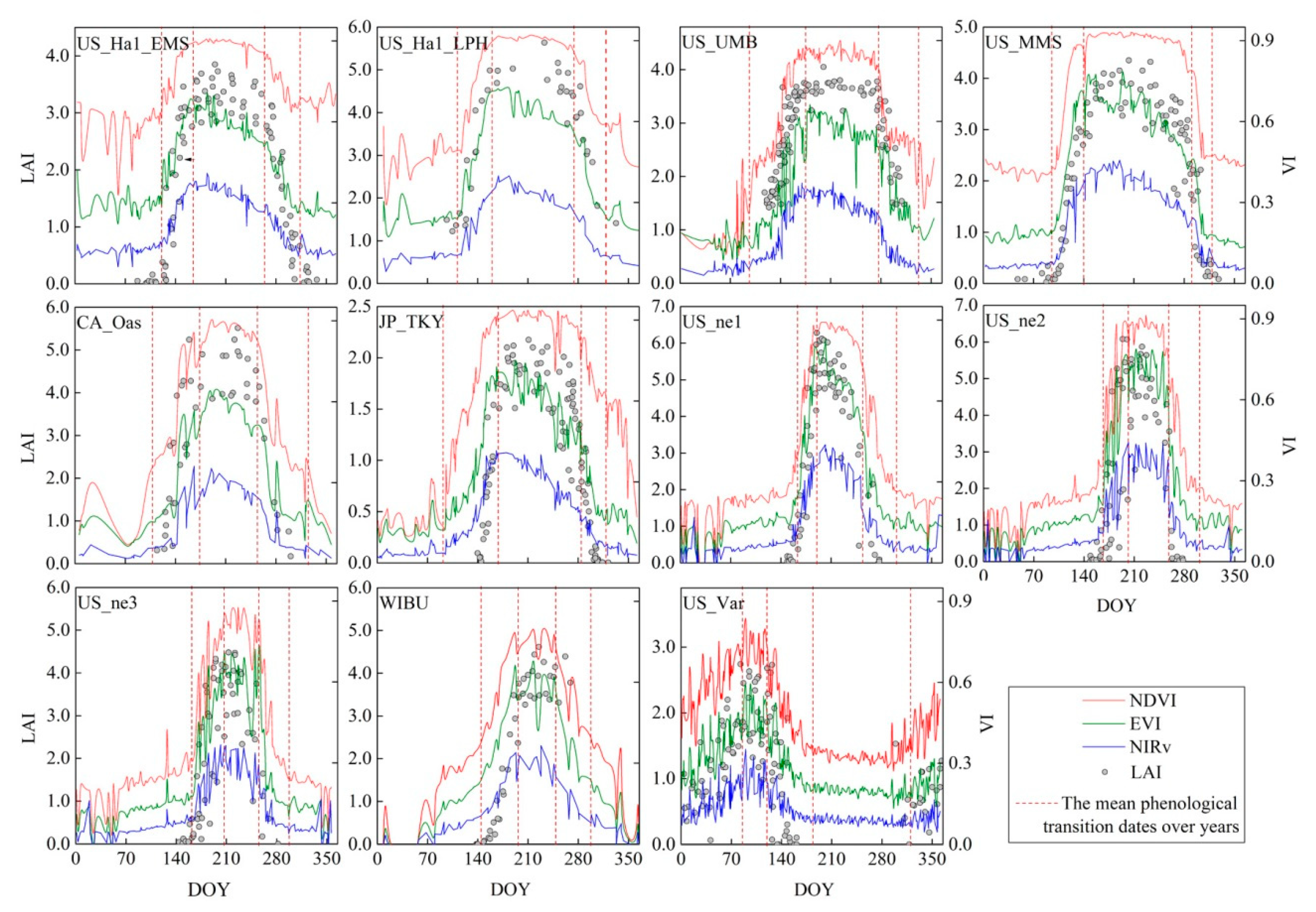
The LAI, NDVI, EVI and NIRv generally exhibited similar temporal profiles for each site (Figure 1), except for the differences in the amplitude and width of the temporal profile curves. The LAI temporal profile of each site corresponded well to the cycle of vegetation phenology (Figure 1, Table 2), which can be distinguished as three phenophases: the growing, flourishing and declining periods.
The growing period of the deciduous forests (the first six subfigures in Figure 1) was generally from early April to early June (DOY 102–159), while that of the crops (the 7th to 10th subfigures in Figure 1) was from early June to mid-July (DOY 153–191), and that of the only grasslands site, US_Var (the last subfigure in Figure 1), was from early November to late March (DOY 310–85). The leaves grew rapidly and began to overlap each other during this period. At the same time, the LAI values increased almost linearly from 0 to 1 to approximately 3 to 5.
The flourishing period of the deciduous forests was from early June to late September (DOY 159–263), while that of the crops was generally from mid-July to early September (DOY 191–244), and that of the US_VAR was very short from late March to late April (DOY 85–118). The leaves continued to grow until reaching crown closure during this period. The number and size of the leaves reached the maximum, and the LAI profile showed a low bow-shape curve.
In the declining period, the number and chlorophyll contents of the leaves decreased continuously from late September to early November (DOY 263–310) for the deciduous forests, while senescence occurred from early September to mid-October (DOY 244–288) for the crops and from late April to late May (DOY 118–178) for the US_Var site. The LAI decreased almost linearly during this period.
3.2. Differences Between the LAIs Estimated with the LAI-VI Relationships Based on Different Phenophases and Those Based on the Entire Vegetation Active Period
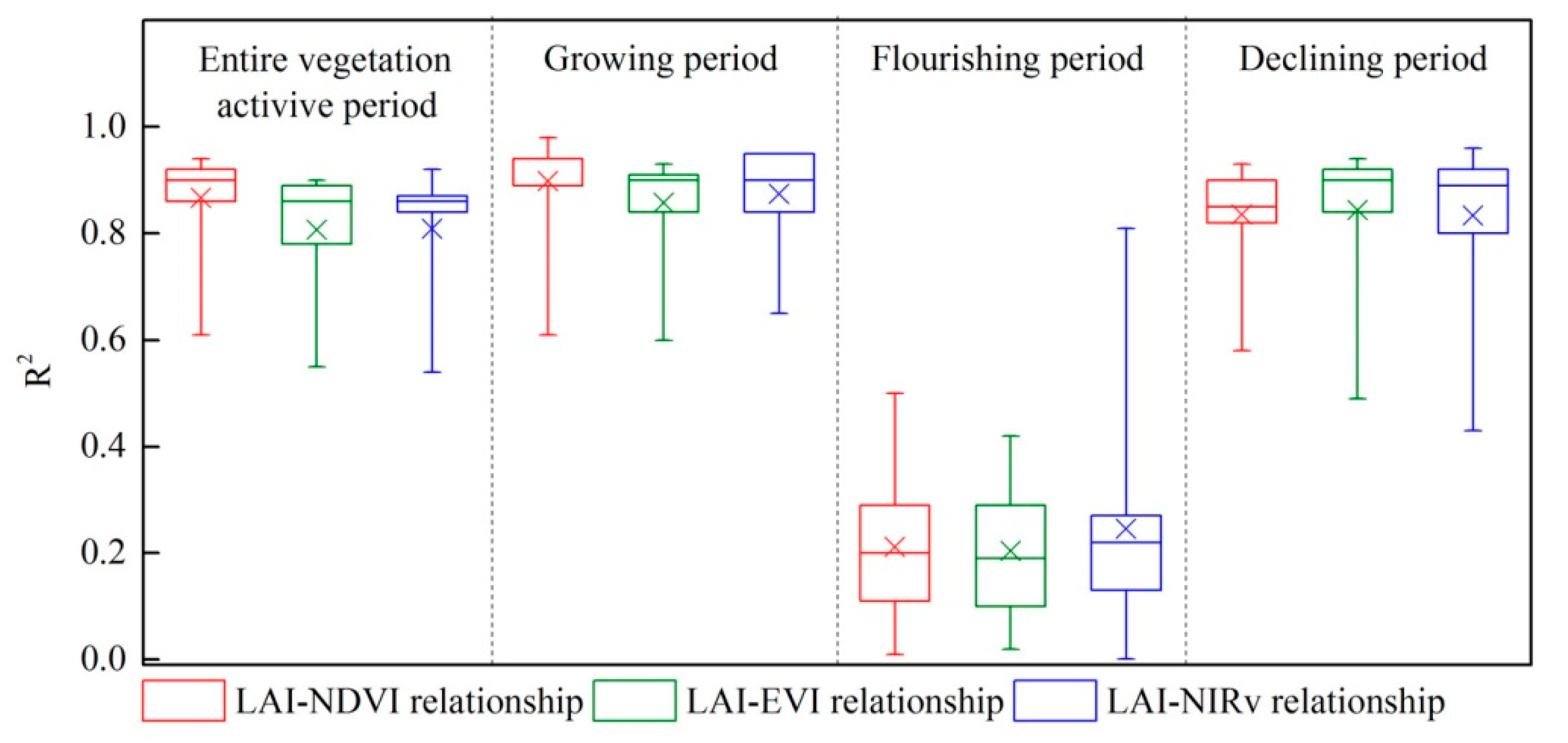
The quadratic polynomial relationship was the best-fitted LAI-VI relationship both for the entire vegetation active period and for the different phenophases. For the entire vegetation active period, all the LAI-VI relationships at 11 sites were significant with R2 = 0.61–0.94 for NDVI, R2 = 0.55–0.9 for EVI and R2 = 0.54–0.92 for NIRv (Figure 2). For the different phenophases, significant LAI-VI relationships were observed during the growing period with R2 = 0.61–0.98 for NDVI, R2 = 0.6–0.93 for EVI and R2 = 0.65–0.95 for NIRv. Their R2 values were the highest among the four periods (i.e., the entire vegetation active, growing, flourishing and declining periods). All the LAI-VI relationships possessed the lowest R2 values during the flourishing period, and the relationships between the LAI and VI remained significant at only a few sites. Significant LAI-VI relationships also occurred during the declining period with R2 = 0.58–0.93 for NDVI, R2 = 0.49–0.94 for EVI and R2 = 0.43–0.96 for NIRv.
The LAIs estimated with the piecewise LAI-VI relationships were better matched to the observed LAIs than those estimated with the single LAI-VI relationship for the entire vegetation active period (Figure 3, Supplementary Materials, Figures S1 and S2). At the beginning and the end of the vegetation active period, some LAI values were overestimated or underestimated by the single LAI-VI relationship based on the entire vegetation active period, whereas the overestimations or underestimations were reduced by the piecewise LAI-VI relationships. The accuracies of the LAIs estimated with the piecewise LAI-VI relationships based on three phenophases were significantly higher than those estimated with the single LAI-VI relationship for the entire vegetation active period (Figure 4, Supplementary Materials, Figures S3 and S4). The maximum differences in the RMSEs for the LAIs estimated with these two methods were 0.24 (based on the NDVI), 0.40 (based on the EVI) and 0.34 (based on the NIRv). Over the entire vegetation active period, the mean RMSE ± standard deviation (SD) value for the LAIs estimated with the piecewise LAI-VI relationships was 0.38 ± 0.13 (based on the NDVI), 0.41 ± 0.13 (based on the EVI) and 0.41 ± 0.14 (based on the NIRv). In comparison, it was 0.46 ± 0.13 (based on the NDVI), 0.55 ± 0.15 (based on the EVI) and 0.55 ± 0.15 (based on the NIRv) for those estimated with a single LAI-VI relationship.
During the growing period, the LAIs estimated with the growing period-based LAI-VI relationship were more accurate than those estimated based on the LAI-VI relationship for the entire vegetation active period. The mean RMSE ± SD value for the former was 0.30 ± 0.11 (based on the NDVI), 0.37 ± 0.11 (based on the EVI) and 0.36 ± 0.13 (based on the NIRv), while it was 0.39 ± 0.11 (based on the NDVI), 0.56 ± 0.14 (based on the EVI) and 0.55 ± 0.14 (based on the NIRv) for the latter.
During the flourishing period, the mean RMSE ± SD value for the LAIs estimated with the flourishing period-based LAI-VI relationship was 0.40 ± 0.14 (based on the NDVI), 0.42 ± 0.14 (based on the EVI) and 0.40 ± 0.15 (based on the NIRv). In comparison, it was 0.48 ± 0.18 (based on the NDVI), 0.58 ± 0.19 (based on the EVI) and 0.54 ± 0.19 (based on the NIRv) for those estimated based on the LAI-VI relationship for the entire vegetation active period.
During the declining period, the LAIs estimated with the declining period-based LAI-VI relationship were also more accurate than those estimated based on the LAI-VI relationship for the entire vegetation active period. The mean RMSE ± SD value for the former was 0.45 ± 0.16 (based on the NDVI), 0.43 ± 0.23 (based on the EVI) and 0.45 ± 0.25 (based on the NIRv), while it was 0.52 ± 0.17 (based on the NDVI), 0.52 ± 0.20 (based on the EVI) and 0.55 ± 0.22 (based on the NIRv) for the latter.
The LAIs estimated with the piecewise LAI-VI relationships were all significantly more accurate than those estimated with the single LAI-VI relationship, regardless of whether they were for different phenophases or for the entire vegetation active period.
3.3. Differences Between the LAIs Estimated with the Three VIs for Different Phenophases
Over the entire vegetation active period, the R2 values for the LAI-NDVI relationships were significantly higher than those for the other two LAI-VI relationships, and the R2 values for the LAI-EVI relationships and LAI-NIRv relationships were similar. The mean R2 ± SD value for the LAI-NDVI relationships, LAI-EVI relationships and LAI-NIRv relationships was 0.87 ± 0.09, 0.81 ± 0.13 and 0.81 ± 0.13, respectively (Figure 2). The mean RMSE ± SD value for the LAI-NDVI relationships, LAI-EVI relationships and LAI-NIRv relationships was 0.46 ± 0.13, 0.55 ± 0.15 and 0.55 ± 0.15, respectively.
During the growing period, the mean R2 ± SD value for the LAI-NDVI relationships, LAI-EVI relationships and LAI-NIRv relationships was 0.90 ± 0.10, 0.86 ± 0.09 and 0.87 ± 0.09, respectively, showing that the LAI-NDVI relationship was significantly stronger than the other two LAI-VI relationships. In addition, the mean RMSE ± SD value for the estimated LAIs was 0.30 ± 0.11 (LAI-NDVI relationships), 0.37 ± 0.11 (LAI-EVI relationships) and 0.36 ± 0.13 (LAI-NIRv relationships), respectively, indicating the NDVI produced significantly better LAI estimations than the EVI and NIRv during the growing period (Figure 5).
During the flourishing period, all the three VIs (NDVI, EVI and NIRv) had poor performances in estimating the LAI, and there was not a stable optimal VI for the LAI estimations. The mean R2 ± SD value for the LAI-NDVI relationships, LAI-EVI relationships and LAI-NIRv relationships was 0.21 ± 0.14, 0.20 ± 0.12 and 0.25 ± 0.21, respectively. The mean RMSE ± SD value for the estimated LAIs was 0.40 ± 0.14 (LAI-NDVI relationships), 0.42 ± 0.14 (LAI-EVI relationships) and 0.40 ± 0.15 (LAI-NIRv relationships), respectively.
During the declining period, the three VIs had the similar performances. However, the LAI-EVI relationship was slightly stronger than the other two LAI-VI relationships at most sites (p > 0.05). The mean R2 ± SD value for the LAI-NDVI relationships, LAI-EVI relationships and LAI-NIRv relationships was 0.84 ± 0.09, 0.85 ± 0.13 and 0.83 ± 0.15, respectively. Moreover, the mean RMSE ± SD value for the estimated LAIs was 0.45 ± 0.16 (LAI-NDVI relationships), 0.43 ± 0.23 (LAI-EVI relationships) and 0.45 ± 0.25 (LAI-NIRv relationships), respectively, indicating the EVI produced slightly better LAI estimations than the other two VIs at most sites during the declining period (p > 0.05).
From the above results, we found that the NDVI was the most stable VI for LAI estimations in the entire vegetation active period, and the EVI and NIRv had similar performance in estimating LAI. However, the LAIs estimated with the NDVI were more accurate than those estimated with the other two VIs during the growing period. In contrast, the LAIs estimated with the EVI had higher accuracies during the declining period. Then, the optimal VI (NDVI, EVI or NIRv) in each phenophase was used for estimating LAI. The estimation accuracies for the piecewise LAI-VI relationships using an optimal VI in each phenophase were significantly higher than those using a single VI in all three phenophases (Figure 6). The mean RMSE ± SD value for the LAIs estimated with the piecewise LAI-VI relationships using an optimal VI in each phenophase was 0.35 ± 0.14. In comparison, it was 0.38 ± 0.14, 0.41 ± 0.15 and 0.42 ± 0.14, respectively, for those estimated with the single NDVI, EVI and NIRv in all three phenophases.
4. Discussion
4.1. LAI Estimation with the Piecewise LAI-VI Relationships Based on Phenophases Versus That with a Single LAI-VI Relationship for the Entire Vegetation Active Period
The LAI and VIs generally showed similar seasonal variations throughout the year, corresponding to the cycle of the vegetation phenology. Previous studies have also noted that the seasonal changes for the VI were closely related to the phenological cycle of the LAI [33,34,35]. Nevertheless, the LAI-VI relationships varied among the phenophases of vegetation. Significant LAI-VI relationships were observed during the growing period and declining period, and they showed an almost linear trend. However, weak relationships between the LAI and VI occurred during the flourishing period due to the saturation of the VI values at high LAI values when the leaves were quite dense [9,36].
The piecewise LAI-VI relationships based on phenophases can better reflect the leaf phenological cycle than the single LAI-VI relationship for the entire vegetation active period. Consequently, the LAIs estimated with the piecewise LAI-VI relationships were better matched to the observed LAIs than those estimated with the single LAI-VI relationship. Thus, the accuracies of the LAIs estimated based on the piecewise LAI-VI relationships were significantly higher than those estimated based on the single LAI-VI relationship (Figure 2, Figure 3 and Figure 4, Supplementary Materials, Figures S1–4). Potithep et al. confirmed that the two-period LAI-VI relationship can better represent the seasonal variations of the LAI and VI than the one-period relationship; thus, the two-period LAI-VI relationship could obtain more accurate LAI estimations [8]. Wang et al. [9] and Xin et al. [37] also proved the necessities and advantages of piecewise LAI-VI relationships for LAI estimations. The LAI-VI relationships varied with the progressing phenology of the vegetation, and the effects of leaf phenology on LAI estimations were taken into account in the piecewise LAI-VI relationships. Thus, we suggest using piecewise LAI-VI relationships based on three phenophases instead of a single LAI-VI relationship for LAI estimations.
The LAI estimations based on the single LAI-VI relationship were overestimated or underestimated at the beginning and end of the growing season. Although the overestimations or underestimations were reduced by the piecewise LAI-VI relationships, it still existed. This may be due to the few leaves in the canopy at the beginning and end of the growing season. Thus, the spectral information of floor vegetation and soil is partly reflected by the VI values [38], which in turn affects the LAI estimations.
4.2. Performances of the Three VIs in Estimating the LAI for Different Phenophases
The seasonal profiles of the three VIs were similar to that of the LAI, whereas the performances of the VIs in estimating the LAI were different among the phenophases. The LAI estimations based on the NDVI were more accurate than those based on the other two VIs during the growing period, which was consistent with the results of Wang et al. [9]. The leaves of the canopy begin to develop during this period, the number of leaves increases rapidly, and at the same time, the chlorophyll content increases gradually. The NDVI is sensitive to the change of the chlorophyll content [39], and it is the most stable vegetation index for the LAI estimations; thus, the NDVI produced better LAI estimations than the other two VIs during the growing period. During the flourishing period, the number and size of the leaves reach the maximum, and the leaves overlap with each other. All of the three VIs had poor performances for the LAI estimations during this period, as the three VIs tend to be saturated in the case of high LAI values. The LAI estimations based on the EVI were slightly more accurate than those based on the other two VIs at most sites during the declining period, which is a little different from the study results of Wang et al. [9]. They found that the relationship between the LAI and MODIS EVI was poor during the leaf senescence period. Given the limited data of an individual year in their study, the results had some uncertainties and may be inappropriate. However, our result was consistent with that of Potithep et al., who found that the EVI produced better LAI estimations than the NDVI during the declining period [8]. The EVI is sensitive to dense vegetation and small changes in chlorophyll content at the beginning of the declining period, when the leaf density is relatively high, but the leaf color begins to change from green to yellow. Further, the EVI is able to respond to the changes in canopy structure rapidly [39], and its use can reduce the background signal and atmospheric influences when the leaves fall off gradually and the chlorophyll content decreases sharply [19,27], such as in the latter half of the declining period. However, the performance of the EVI was not very stable, while the NIRv performed better than the EVI at a few sites because the NIRv can isolate the vegetated signal and eliminate much of the mixed-pixel problem [20].
The LAIs estimated with the piecewise LAI-VI relationships using the optimal VI in each phenophase were significantly more accurate than those using a single VI in all three phenophases. This result is consistent with that of Tillack et al., who reported that different VIs correlated best to the LAI during different phenological periods for black alder forests [10]. They suggested using different VIs for LAI estimations during different phenological periods. He et al. also suggested that different VIs should be used for estimating the LAI at different development stages of winter wheat, taking full advantage of the VI characteristics at different development stages [26].
4.3. Uncertainties, Limitations and Potential Applications
The seasonal relationship between the LAI and VI is affected by diverse factors [40,41,42], such as the leaf optics, sampling strategy, spatial heterogeneity of the sites, canopy structure, sun-sensor geometry and illumination condition. For example, Raabe et al. revealed the leaf inclination angle distribution was the most variable in spring and remains comparatively constant throughout the remainder of the growing season [43]. Weiss et al. pointed out that spatial sampling was a key issue when performing LAI ground measurements that need to be representative of the whole canopy [44], and an optimal sampling strategy can reduce the uncertainties of the LAI-VI relationship caused by spatial heterogeneity [45]. Besides, the impact of sun-sensor geometry on VI was evaluated in this study, the VI product (MOD13Q1) and the VI estimated with the MOCD43A4 product were well correlated (Supplementary Materials, Figure S5). Although these factors have some influences on the seasonal LAI-VI relationship, they are not the most important factors. The seasonal variation of LAI-VI relationship is mainly controlled by the seasonal change of leaf chlorophyll content as proven by other researchers [46]. Xie et al. proved that the canopy reflectance was a complex signal affected by many factors, but the chlorophyll content had much larger impact than other factors, and most variations in canopy reflectance can be explained by the variations in chlorophyll content [47]. Therefore, the seasonal variation of chlorophyll content contributes most to the seasonal variation of LAI-VI relationship. Nevertheless, if the impact from other factors could be reduced, the LAI-VI relationship can be potentially further improved as well.
The piecewise LAI-VI relationships proposed in this study can improve the estimation accuracy of LAI effectively, but it is necessary to know the vegetation type of the study area in advance when using the piecewise LAI-VI relationships, which may limit the practical applications of the method. Besides, only the relationships between the LAI and the three representative VIs (i.e., NDVI, EVI and NIRv) in two vegetation types were investigated in this study, due to the limitation of data availability. In the future, under the support of large amounts of observed data (such as the existing FLUXNET database, LTER database, CERN database and NEON database), a look up table (LUT) of piecewise LAI-VI relationships incorporating the phenological information of diverse vegetation types may be constructed to produce consistent LAI products of high quality and long time series. In addition, more VIs should be taken into account in further study, especially the VI constructed with the red edge channel, such as the red edge normalized difference vegetation index (NDVI-RE) [48,49], CIRed-edge [50], modified red edge simple ratio (mSR-RE) [49,51] and MERIS terrestrial chlorophyll index (MTCI) [52], as the red edge can produce a positive response to small changes in spectral reflectance, especially in terms of a small decrease or increase in the LAI [10,29]. The use of red edge can partly overcome the saturation of most VIs under high LAI values [53,54], which is a problem particularly occurring during the flourishing period.
Currently, the main algorithm of MODIS LAI products uses a fixed leaf spectrum for each biome across the whole season, and in addition, the backup algorithm uses a single LAI-NDVI relationship. The phenological information of vegetation and seasonal change of leaf optics (e.g., leaf chlorophyll content and reflectance) have not been considered in both of the algorithms [55]. Besides, only a single VI (NDVI) is used in the backup algorithm, which may further bring bias to the MODIS LAI products [56]. Whereas, the piecewise LAI-VI relationships proposed in this study were established by using the optimal VI in each phenophase, which may be able to overcome some of the problems in the algorithms for the MODIS LAI products since they take full advantage of phenological information and leaf optics. Furthermore, our study strengthens the impact of seasonal variation of leaf chlorophyll content on the LAI estimations.
5. Conclusions
The observed LAI data and MODIS VI products at 11 sites (six deciduous forests sites, four crop sites and one grasslands site) were collected to investigate the LAI-VI relationships in different phenophases and for different VIs (i.e., NDVI, EVI and NIRv). The LAI-VI relationships differed among phenophases. Significant LAI-VI relationships were observed during the growing period and declining period, and they showed an almost linear trend, whereas weak LAI-VI relationships occurred during the flourishing period. The piecewise LAI-VI relationships based on phenophases can better reflect the leaf phenological cycle than the single LAI-VI relationship for the entire vegetation active period. Consequently, the accuracies for LAIs estimated with the piecewise LAI-VI relationships were significantly higher than those estimated with the single LAI-VI relationship. In addition, the performances of the three VIs in estimating the LAI also varied among phenophases. The NDVI produced significantly better LAI estimations than the other two VIs during the growing period, while the EVI produced slightly better estimations than the other two VIs in most sites during the declining period (p > 0.05). However, the performance of the EVI was not very stable, the NIRv performed better than the EVI at a few sites during the declining period. All the three VIs had poor performances in estimating the LAI during the flourishing period.
The piecewise LAI-VI relationships based on phenophases and the optimal VIs for different phenophases were recommended for estimating the LAI. The piecewise LAI-VI relationships established in this study were simple and feasible, and they may be applied to operational applications in the future to produce consistent LAI products of high quality and long time series. These LAI products can be further used for drought monitoring, crop growth monitoring, productivity estimation, ecological assessment and carbon cycle research.
Supplementary Materials
The following are available online at https://www.mdpi.com/2072-4292/11/6/689/s1, Figure S1: Scatter plots of the observed LAIs versus the LAIs estimated with the piecewise LAI-enhanced vegetation index (EVI) relationships (red solid circle) and the single LAI-EVI relationship (black open circle), Figure S2: Scatter plots of the observed LAIs versus LAIs estimated with the piecewise LAI-near-infrared reflectance of vegetation (NIRv) relationships (red solid circle) and the single LAI-EVI relationship (black open circle), Figure S3: The RMSEs for the LAIs estimated based on the LAI-EVI relationships for the entire vegetation active period and for the different phenophases, Figure S4: The RMSEs for the LAIs estimated based on the LAI-NIRv relationships for the entire vegetation active period and for the different phenophases, Figure S5: Scatter plots of the NDVI product (MOD13Q1) versus the NDVI estimated with the MOCD43A4 product, Table S1. Results of the regression analysis, F-test and RMSE of the LAI-VI relationships during the entire vegetation active period and different phenophases.
Author Contributions
Conceptualization, K.Q. and W.Z.; methodology, K.Q. and W.Z.; formal analysis, K.Q.; writing—original draft preparation, K.Q.; writing—review and editing, K.Q., W.Z., Z.X., and P.L.; visualization, Z.X., and P.L.
Funding
This research was funded by National Natural Science Foundation of China (No. 41771047) and the State Key Laboratory of Earth Surface Processes and Resource Ecology (No. 2017-FX-01(1)).
Acknowledgments
We thank FLUXNET PIs, JLTER PIs and LTER PIs who provided the data on which our analysis was based.
Conflicts of Interest
The authors have no conflicts of interest to declare.
References
- Breda, N.J.J. Ground-based measurements of leaf area index: A review of methods, instruments and current controversies. J. Exp. Bot. 2003, 54, 2403–2417. [Google Scholar] [CrossRef] [PubMed]
- Battaglia, M.; Sands, P.; White, D.; Mummery, D. CABALA: A linked carbon, water and nitrogen model of forest growth for silvicultural decision support. For. Ecol. Manag. 2004, 193, 251–282. [Google Scholar] [CrossRef]
- Chapin, F.S.; Woodwell, G.M.; Randerson, J.T.; Rastetter, E.B.; Lovett, G.M.; Baldocchi, D.D.; Clark, D.A.; Harmon, M.E.; Schimel, D.S.; Valentini, R.; et al. Reconciling carbon-cycle concepts, terminology, and methods. Ecosystems 2006, 9, 1041–1050. [Google Scholar] [CrossRef]
- Fan, W.; Liu, Y.; Xu, X.; Chen, G.; Zhang, B. A new FAPAR analytical model based on the law of energy conservation: A case study in China. IEEE J. Sel. Top. Appl. Earth Obs. Remote Sens. 2014, 7, 3945–3955. [Google Scholar] [CrossRef]
- Tian, Y.; Zheng, Y.; Zheng, C.; Xiao, H.; Fan, W.; Zou, S.; Wu, B.; Yao, Y.; Zhang, A.; Liu, J. Exploring scale-dependent ecohydrological responses in a large endorheic river basin through integrated surface water-groundwater modeling. Water Resour. Res. 2015, 51, 4065–4085. [Google Scholar] [CrossRef] [Green Version]
- Field, C.B.; Avissar, R. Bidirectional interactions between the biosphere and the atmosphere—Introduction. Glob. Chang. Biol. 1998, 4, 459–460. [Google Scholar] [CrossRef]
- Fassnacht, K.S.; Gower, S.T.; Norman, J.M.; Mcmurtric, R.E. A comparison of optical and direct methods for estimating foliage surface area index in forests. Agric. For. Meteorol. 1994, 71, 183–207. [Google Scholar] [CrossRef]
- Potithep, S.; Nagai, S.; Nasahara, K.N.; Muraoka, H.; Suzuki, R. Two separate periods of the LAI–VIs relationships using in situ measurements in a deciduous broadleaf forest. Agric. For. Meteorol. 2013, 169, 148–155. [Google Scholar] [CrossRef]
- Wang, Q.; Adiku, S.; Tenhunen, J.; Granier, A. On the relationship of NDVI with leaf area index in a deciduous forest site. Remote Sens. Environ. 2005, 94, 244–255. [Google Scholar] [CrossRef]
- Tillack, A.; Clasen, A.; Kleinschmit, B.; Förster, M. Estimation of the seasonal leaf area index in an alluvial forest using high-resolution satellite-based vegetation indices. Remote Sens. Environ. 2014, 141, 52–63. [Google Scholar] [CrossRef]
- Yan, G.J.; Hu, R.H.; Luo, J.H.; Mu, X.H.; Xie, D.H.; Zhang, W.M. Eview of indirect methods for leaf area index measurement. J. Remote Sens. 2016, 20, 958–978. (In Chinese) [Google Scholar]
- Chen, P.Y.; Fedosejevs, G.; Tiscareño-López, M.; Arnold, J.G. Assessment of MODIS-EVI, MODIS-NDVI and VEGETATION-NDVI composite data using agricultural measurements: An example at corn fields in western Mexico. Environ. Monit. Assess. 2006, 119, 69–82. [Google Scholar] [CrossRef] [PubMed]
- He, L.H.; Chu, K.H.; Xiao, X.M. The relationship of vegetaion-derived index and site-measured rice LAI. J. Remote Sens. 2004, 8, 672–676. (In Chinese) [Google Scholar]
- Kobayashi, H.; Suzuki, R.; Kobayashi, S. Reflectance seasonality and its relation to the canopy leaf area index in an eastern Siberian larch forest: Multi-satellite data and radiative transfer analyses. Remote Sens. Environ. 2007, 106, 238–252. [Google Scholar] [CrossRef]
- Sun, P.S.; Liu, S.R.; Liu, J.T.; Li, C.W.; Lin, Y.; Jiang, H. Derivation and validation of leaf area index maps using NDVI data of different resolution satellite imageries. Acta Ecol. Sin. 2006, 26, 3826–3924. (In Chinese) [Google Scholar]
- Birky, A.K. NDVI and a simple model of deciduous forest seasonal dynamics. Ecol. Model. 2001, 143, 43–58. [Google Scholar] [CrossRef]
- Cheng, Q.; Huang, J.F.; Wang, R.C.; Tang, Y.L. Analyses of the correlation between rice LAI and simulated MODIS vegetation indices, red edge position. Trans. Csae 2003, 19, 104–108. (In Chinese) [Google Scholar]
- Gu, Y.; Wylie, B.K.; Howard, D.M.; Phuyal, K.P.; Ji, L. NDVI saturation adjustment: A new approach for improving cropland performance estimates in the Greater Platte River Basin, USA. Ecol. Indic. 2013, 30, 1–6. [Google Scholar] [CrossRef]
- Huete, A.; Didan, K.; Miura, T.; Rodriguez, E.P.; Gao, X.; Ferreira, L.G. Overview of the radiometric and biophysical performance of the MODIS vegetation indices. Remote Sens. Environ. 2002, 83, 195–213. [Google Scholar] [CrossRef]
- Badgley, G.; Field, C.B.; Berry, J.A. Canopy near-infrared reflectance and terrestrial photosynthesis. Sci. Adv. 2017, 3, e1602244. [Google Scholar] [CrossRef] [Green Version]
- Kross, A.; Mcnairn, H.; Lapen, D.; Sunohara, M.; Champagne, C. Assessment of RapidEye vegetation indices for estimation of leaf area index and biomass in corn and soybean crops. Int. J. Appl. Earth Obs. Geoinf. 2015, 34, 235–248. [Google Scholar] [CrossRef] [Green Version]
- Nguy-Robertson, A.L.; Peng, Y.; Gitelson, A.A.; Arkebauer, T.J.; Pimstein, A.; Herrmann, I.; Karnieli, A.; Rundquist, D.C.; Bonfil, D.J. Estimating green LAI in four crops: Potential of determining optimal spectral bands for a universal algorithm. Agric. For. Meteorol. 2014, 192–193, 140–148. [Google Scholar] [CrossRef]
- Colombo, R.; Bellingeri, D.; Fasolini, D.; Marino, C.M. Retrieval of leaf area index in different vegetation types using high resolution satellite data. Remote Sens. Environ. 2003, 86, 120–131. [Google Scholar] [CrossRef]
- Delegido, J.; Verrelst, J.; Rivera, J.P.; Ruiz-Verdú, A.; Moreno, J. Brown and green LAI mapping through spectral indices. Int. J. Appl. Earth Obs. Geoinf. 2015, 35, 350–358. [Google Scholar] [CrossRef]
- Din, M.; Zheng, W.; Rashid, M.; Wang, S.; Shi, Z. Evaluating hyperspectral vegetation indices for leaf area index estimation of Oryza satival. at diverse phenological stages. Front. Plant Sci. 2017, 8, 1–17. [Google Scholar] [CrossRef] [PubMed]
- He, J.; Liu, B.F.; Li, J. Monitoring model of leaf area index of winter wheat based on hyperspectral reflectance at different growth stages. Trans. Csae 2014, 30, 141–150. (In Chinese) [Google Scholar]
- Didan, K.; Munoz, A.B.; Solano, R.; Huete, A. MODIS Vegetation Index User’s Guide (MOD13 Series). Version 3.00; Vegetation Index and Phenology Lab, The University of Arizona: Tucson, AZ, USA, 2015. [Google Scholar]
- Kharbouche, S.; Muller, J.P. Sea Ice Albedo from MISR and MODIS: Production, Validation, and Trend Analysis. Remote Sens. 2019, 11, 9. [Google Scholar] [CrossRef]
- Viña, A.; Gitelson, A.A.; Nguy-Robertson, A.L.; Peng, Y. Comparison of different vegetation indices for the remote assessment of green leaf area index of crops. Remote Sens. Environ. 2011, 115, 3468–3478. [Google Scholar]
- Chauvenet, W. A Manual of Spherical and Practical Astronomy; J.B. Lippincott Publishers: Philadelphia, PA, USA, 1960. [Google Scholar]
- Rahman, M.S.; Al-Amri, K. Effect of outlier on coefficient of determination. Int. J. Educ. Res. 2011, 6, 9–20. [Google Scholar]
- Zhang, X.; Friedl, M.A.; Schaaf, C.B.; Strahler, A.H.; Hodges, J.C.F.; Gao, F.; Reed, B.C.; Huete, A. Monitoring vegetation phenology using MODIS. Remote Sens. Environ. 2003, 84, 471–475. [Google Scholar] [CrossRef]
- Fang, H.; Li, W.; Wei, S.; Jiang, C. Seasonal variation of leaf area index (LAI) over paddy rice fields in NE China: Intercomparison of destructive sampling, LAI-2200, digital hemispherical photography (DHP), and AccuPAR methods. Agric. For. Meteorol. 2014, 198–199, 126–141. [Google Scholar] [CrossRef]
- Richardson, A.D.; Anderson, R.S.; Arain, M.A.; Barr, A.G.; Bohrer, G.; Chen, G.; Chen, J.M.; Ciais, P.; Davis, K.J.; Desai, A.R.; et al. Terrestrial biosphere models need better representation of vegetation phenology: Results from the North American carbon Program Site Synthesis. Glob. Change Biol. 2012, 18, 566–584. [Google Scholar] [CrossRef]
- Savoy, P.; Mackay, D.S. Modeling the seasonal dynamics of leaf area index based on environmental constraints to canopy development. Agric. For. Meteorol. 2015, 200, 46–56. [Google Scholar] [CrossRef]
- Chen, X.; Vierling, L.; Deering, D.; Conley, A. Monitoring boreal forest leaf area index across a Siberian burn chronosequence: A MODIS validation study. Int. J. Remote Sens. 2005, 26, 5433–5451. [Google Scholar] [CrossRef]
- Xin, Y.M.; Yin, H.; Chen, L.; Zhang, M.L.; Ren, Z.Y.; Miao, J. Estimation of rice canopy LAI with different growth stages based on hyperspectral remote sensing data. Chin. J. Agrometeorol. 2015, 36, 762–768. (In Chinese) [Google Scholar]
- Shin, N.; Kenlonishida, N.; Hiroyuki, M.; Tsuyoshi, A.; Satoshi, T. Field experiments to test the use of the normalized-difference vegetation index for phenology detection. Agric. For. Meteorol. 2010, 150, 152–160. [Google Scholar] [Green Version]
- Xiang, G.; Huete, A.R.; Wenge, N.; Miura, T. Optical-biophysical relationships of vegetation spectra without background contamination. Remote Sens. Environ. 2000, 74, 609–620. [Google Scholar]
- Liu, Z.; Chen, J.M.; Jin, G.; Qi, Y. Estimating seasonal variations of leaf area index using litterfall collection and optical methods in four mixed evergreen-deciduous forests. Agric. For. Meteorol. 2015, 209–210, 36–48. [Google Scholar] [CrossRef]
- Liu, Z.; Jin, G. Bias analysis of seasonal changes of leaf area index derived from optical methods. Sci. Silvae Sin. 2016, 52, 11–21. (In Chinese) [Google Scholar]
- Wang, Q.; Tenhunen, J.; Dinh, N.Q.; Reichstein, M.; Otieno, D.; Granier, A.; Pilegarrd, K. Evaluation of seasonal variation of MODIS derived leaf area index at two European deciduous broadleaf forest sites. Remote Sens. Environ. 2005, 96, 475–484. [Google Scholar] [CrossRef]
- Raabe, K.; Pisek, J.; Sonnentag, O.; Annuk, K. Variations of leaf inclination angle distribution with height over the growing season and light exposure for eight broadleaf tree species. Agric. For. Meteorol. 2015, 214–215, 2–11. [Google Scholar] [CrossRef]
- Weiss, M.; Baret, F.; Smith, G.J.; Jonckheere, I.; Coppin, P. Review of methods for in situ leaf area index (lai) determination: Part II. estimation of lai, errors and sampling. Agric. For. Meteorol. 2004, 121, 37–53. [Google Scholar] [CrossRef]
- Zeng, Y.; Li, J.; Liu, Q.; Li, L.; Xu, B.; Yin, G.; Peng, J. A sampling strategy for remotely sensed lai product validation over heterogeneous land surfaces. IEEE J. Sel. Top. Appl. Earth Obs. Remote Sens. 2014, 7, 3128–3142. [Google Scholar] [CrossRef]
- Yang, F.; Sun, J.; Fang, H.; Yao, Z.; Zhang, J.; Zhu, Y.; Song, K.; Wang, Z.; Hu, M. Comparison of different methods for corn lai estimation over northeastern china. Int. J. Appl. Earth Obs. Geoinf. 2012, 18, 462–471. [Google Scholar]
- Xie, Q.; Dash, J.; Huang, W.; Peng, D.; Qin, Q.; Mortimer, H.; Casa, R.; Pignatti, S.; Laneve, G.; Pascucci, S.; et al. Vegetation indices combining the red and red-edge spectral information for leaf area index retrieval. IEEE J. Sel. Top. Appl. Earth Obs. Remote Sens. 2018, 11, 1–12. [Google Scholar] [CrossRef]
- Gitelson, A.; Merzlyak, M.N. Spectral reflectance changes associated with autumn senescence of Aesculus hippocastanum L. and Acer platanoides L. leaves. Spectral features and relation to chlorophyll Estimation. J. Plant Physiol. 1994, 143, 286–292. [Google Scholar] [CrossRef]
- Sims, D.A.; Gamon, J.A. Relationships between leaf pigment content and spectral reflectance across a wide range of species, leaf structures and developmental stages. Remote Sens. Environ. 2002, 81, 337–354. [Google Scholar] [CrossRef]
- Gitelson, A.A.; Viña, A.; Arkebauer, T.J.; Rundquist, D.C.; Keydan, G.; Leavitt, B. Remote estimation of leaf area index and green leaf biomass in maize canopies. Geophys. Res. Lett. 2003, 30. [Google Scholar] [CrossRef] [Green Version]
- Datt, B. A new reflectance index for remote sensing of chlorophyll content in higher plants: Tests using Eucalyptus leaves. J. Plant Physiol. 1999, 154, 30–36. [Google Scholar] [CrossRef]
- Dash, J.; Curran, P.J. The MERIS terrestrial chlorophyll index. Int. J. Remote Sens. 2004, 25, 5403–5413. [Google Scholar] [CrossRef]
- Eitel, J.U.H.; Vierling, L.A.; Litvak, M.E.; Long, D.S.; Schulthess, U.; Ager, A.A.; Krofcheck, D.J.; Stoscheck, L. Broadband, red-edge information from satellites improves early stress detection in a New Mexico conifer woodland. Remote Sens. Environ. 2011, 115, 3640–3646. [Google Scholar] [CrossRef]
- Schuster, C.; Kleinschmit, B. Testing the red edge channel for improving land-use classifications based on high-resolution multi-spectral satellite data. Int. J. Remote Sens. 2012, 33, 5583–5599. [Google Scholar] [CrossRef]
- Yang, W.; Huang, D.; Tan, B.; Stroeve, J.C.; Shabanov, N.V.; Knyazikhin, Y.; Nemani, R.R.; Myneni, R.B. Analysis of leaf area index and fraction of PAR absorbed by vegetation products from the terra MODIS sensor: 2000–2005. IEEE Trans. Geosci. Remote Sens. 2006, 44, 1829–1842. [Google Scholar] [CrossRef]
- Shabanov, N.V.; Dong, H.; Wenze, Y.; Tan, B.; Knyazikhin, Y.; Myneni, R.B.; Ahl, D.E.; Gower, S.T.; Huete, A.R.; Aragao, L.E.O.C.; et al. Analysis and optimization of the MODIS leaf area index algorithm retrievals over broadleaf forests. IEEE Trans. Geosci. Remote Sens. 2005, 43, 1855–1865. [Google Scholar] [CrossRef] [Green Version]
Figure 1.
The leaf area index (LAI) and vegetation index (VI) profiles marked with four mean phenological transition dates over the years. The red vertical dashed lines from the left to right are green-up, maturity, senescence and dormancy (for the US_Var site, the red vertical dashed lines represent maturity, senescence, dormancy and green-up from the left to right).

Figure 2.
The R2 of the best-fitted LAI-VI relationships for the entire vegetation active period and for the different phenophases. The bottoms and tops of the boxes are the 25th and 75th percentiles; the bands near the middle are the median; the ends of the whiskers represent the minimum and maximum; and the crosses designate the mean value.

Figure 3.
Scatter plots of the observed LAIs versus LAIs estimated with the piecewise LAI-normalized difference vegetation (NDVI) relationship (red solid circle) and the single LAI-NDVI relationship (black open circle).
Figure 3.
Scatter plots of the observed LAIs versus LAIs estimated with the piecewise LAI-normalized difference vegetation (NDVI) relationship (red solid circle) and the single LAI-NDVI relationship (black open circle).

Figure 4.
The root-mean-square errors (RMSEs) for the LAIs estimated based on a single LAI-NDVI relationship for the entire vegetation active period and those based on the piecewise LAI-NDVI relationships for different phenophases. See Figure 2 for descriptions of the boxplot.
Figure 4.
The root-mean-square errors (RMSEs) for the LAIs estimated based on a single LAI-NDVI relationship for the entire vegetation active period and those based on the piecewise LAI-NDVI relationships for different phenophases. See Figure 2 for descriptions of the boxplot.

Figure 5.
The RMSEs of the LAIs estimated with the three LAI-VI relationships for different phenophases. See Figure 2 for descriptions of the boxplot.
Figure 5.
The RMSEs of the LAIs estimated with the three LAI-VI relationships for different phenophases. See Figure 2 for descriptions of the boxplot.

Figure 6.
The RMSEs of the LAIs estimated based on the piecewise LAI-VI relationships using a single VI in the three phenophases and those using the optimal VI in each phenophase. See Figure 2 for descriptions of the boxplot.
Figure 6.
The RMSEs of the LAIs estimated based on the piecewise LAI-VI relationships using a single VI in the three phenophases and those using the optimal VI in each phenophase. See Figure 2 for descriptions of the boxplot.


Table 1.
Site locations, characteristics, and years of data availability.
| Site Name (Site ID) | Country | Long. °E | Lat. °N | Elevation (m) | Vegetation Type | Vegetation Height (m) | Acquisition Approach of LAI Data | Years of Data Available |
|---|---|---|---|---|---|---|---|---|
| Harvard forest EMS Tower (US_Ha1_EMS) | America | −72.17 | 42.54 | 340 | Deciduous forest | 23 | LAI-2000 | 2006–2013 |
| Harvard forest LPH Tower (US_Ha1_LPH) | America | −72.18 | 42.53 | 345 | Deciduous forest | 23 | LAI-2000 | 2007–2010 |
| Univ. of Mich. Biological Station (US_UMB) | America | −84.71 | 45.56 | 243 | Deciduous forest | 22 | LAI-2000 | 2001–2013 |
| Morgan Monroe State Forest (US_MMS) | America | −86.41 | 39.32 | 275 | Deciduous forest | 25–27 | LAI-2000 | 2001–2006 |
| SK-Old Aspen (CA_Oas) | Canada | −106.20 | 53.63 | 601 | Deciduous forest | 21.5 | LAI 2000 + TRAC | 2001–2004 |
| Takayama deciduous broadleaf forest (JP_TKY) | Japan | 137.42 | 36.15 | 1420 | Deciduous forest | 15–20 | Litterfall collection | 2005–2014 |
| Mead-irrigated continuous maize site (US_ne1) | America | −96.48 | 41.17 | 361 | Crop | - | LI-COR Area Meter | 2001–2007 |
| Mead-irrigated maize-soybean rotation site (US_ne2) | America | −96.47 | 41.16 | 362 | Crop | - | LI-COR Area Meter | 2001–2007 |
| Mead-rainfed maize-soybean rotation site (US_ne3) | America | −96.44 | 41.18 | 363 | Crop | - | LI-COR Area Meter | 2001–2007 |
| Wibu field site (WIBU) | America | −89.40 | 43.27 | 305 | Crop | - | LAI-2200 | 2012–2014 |
| Vaira Ranch-Ione (US-Var) | America | −120.95 | 38.41 | 129 | Grassland | - | LI-COR Area Meter | 2002–2014 |
Table 2.
The four phenological transition dates of vegetation at each site (mean day of year (DOY) ± standard deviation).
Table 2.
The four phenological transition dates of vegetation at each site (mean day of year (DOY) ± standard deviation).
| No. | Site | Green-up | Maturity | Senescence | Dormancy |
|---|---|---|---|---|---|
| 1 | US_Ha1_EMS | 117 ± 12 | 159 ± 7 | 254 ± 9 | 301 ± 11 |
| 2 | US_Ha1_LPH | 110 ± 7 | 156 ± 4 | 265 ± 7 | 308 ± 2 |
| 3 | US_UMB | 96 ± 8 | 169 ± 12 | 264 ± 10 | 321 ± 12 |
| 4 | US_MMS | 95 ± 9 | 134 ± 9 | 279 ± 4 | 306 ± 7 |
| 5 | CA_Oas | 106 ± 5 | 172 ± 9 | 241 ± 4 | 316 ± 4 |
| 6 | JP_TKY | 89 ± 7 | 164 ± 9 | 274 ± 8 | 310 ± 5 |
| 7 | US_ne1 | 156 ± 4 | 182 ± 6 | 244 ± 4 | 289 ± 10 |
| 8 | US_ne2 | 160 ± 6 | 195 ± 16 | 247 ± 4 | 289 ± 9 |
| 9 | US_ne3 | 156 ± 10 | 197 ± 17 | 243 ± 14 | 284 ± 8 |
| 10 | WIBU | 139 ± 7 | 191 ± 3 | 241 ± 4 | 289 ± 9 |
| 11 | US_Var | 310 ± 9 | 85 ± 7 | 118 ± 7 | 178 ± 6 |
© 2019 by the authors. Licensee MDPI, Basel, Switzerland. This article is an open access article distributed under the terms and conditions of the Creative Commons Attribution (CC BY) license (http://creativecommons.org/licenses/by/4.0/).
Share and Cite
MDPI and ACS Style
Qiao, K.; Zhu, W.; Xie, Z.; Li, P. Estimating the Seasonal Dynamics of the Leaf Area Index Using Piecewise LAI-VI Relationships Based on Phenophases. Remote Sens. 2019, 11, 689. https://doi.org/10.3390/rs11060689
AMA Style
Qiao K, Zhu W, Xie Z, Li P. Estimating the Seasonal Dynamics of the Leaf Area Index Using Piecewise LAI-VI Relationships Based on Phenophases. Remote Sensing. 2019; 11(6):689. https://doi.org/10.3390/rs11060689
Chicago/Turabian StyleQiao, Kun, Wenquan Zhu, Zhiying Xie, and Peixian Li. 2019. "Estimating the Seasonal Dynamics of the Leaf Area Index Using Piecewise LAI-VI Relationships Based on Phenophases" Remote Sensing 11, no. 6: 689. https://doi.org/10.3390/rs11060689
Note that from the first issue of 2016, this journal uses article numbers instead of page numbers. See further details here.