Article

Retrieval of Sea Surface Wind Speeds from Gaofen-3 Full Polarimetric Data

1
Key Laboratory of Digital Earth Science, Institute of Remote Sensing and Digital Earth, Chinese Academy of Sciences, Beijing 100094, China
2
University of Chinese Academy of Sciences, Beijing 101408, China
3
Laboratory for Regional Oceanography and Numerical Modeling, Qingdao National Laboratory for Marine Science and Technology, Qingdao 266235, China
4
Hainan Key Laboratory of Earth Observation, Sanya 572029, China
5
Key Laboratory of Space Ocean Remote Sensing and Applications, National Satellite Ocean Application Service, Beijing 100081, China
6
Mailbox No.5111, Beijing 100094, China
*
Author to whom correspondence should be addressed.
Remote Sens. 2019, 11(7), 813; https://doi.org/10.3390/rs11070813
Submission received: 19 February 2019 / Revised: 29 March 2019 / Accepted: 1 April 2019 / Published: 4 April 2019
(This article belongs to the Special Issue Synthetic Aperture Radar Observations of Marine Coastal Environments)

Abstract

:
In this paper, the sea surface wind speed (SSWS) retrieval from Gaofen-3 (GF-3) quad-polarization stripmap (QPS) data in vertical-vertical (VV), horizontal-horizontal (HH), and vertical-horizontal (VH) polarizations is investigated in detail based on 3170 scenes acquired from October 2016 to May 2018. The radiometric calibration factor of the VV polarization data is examined first. This calibration factor generally meets the requirement of SSWS retrieval accuracy with an absolute bias of less than 0.5 m/s but shows highly dispersed characteristics. These results lead to SSWS retrievals with a small bias of 0.18 m/s, but a rather high root mean square error (RMSE) of 2.36 m/s when compared with the ERA-Interim reanalysis model data. Two refitted polarization ratio (PR) models for the QPS HH polarization data are presented. Based on a combination of the incidence angle-dependent and azimuth angle-dependent PR model and CMOD5.N, the SSWS derived from the QPS HH data shows a bias of 0.07 m/s and an RMSE of 2.26 m/s relative to the ERA-Interim reanalysis model wind speed. A linear function relating SSWS and the normalized radar cross section (NRCS) of QPS VH data is derived. The SSWS data retrieved from the QPS VH data show good agreement with the WindSat SSWS data, with a bias of 0.1 m/s and an RMSE of 2.02 m/s. We also apply the linear function to the GF-3 Wide ScanSAR data acquired for the typhoon SOULIK, which yields very good agreement with the model results. A comparison of SSWS retrievals among three different polarization datasets is also presented. The current study and our previous work demonstrate that the general accuracy of the SSWS retrieval based on GF-3 QPS data has an absolute bias of less than 0.3 m/s and an RMSE of 2.0 ± 0.2 m/s relative to various datasets. Further improvement will depend on dedicated radiometric calibration efforts.

1. Introduction

Ocean wind is the major force of global ocean circulation [1] and is typically measured by anemometers onboard buoys, platforms, and ships very close to the sea surface. The most common reference height of ocean wind measurements is 10 m above the sea surface, and this wind is customarily called sea surface wind (SSW). The ocean is vast and dynamic, and SSW exhibits considerable spatial and temporal variations. Consequently, advanced techniques for observing SSW from space, involving both active and passive remote sensors, present different unique advantages.
Spaceborne synthetic aperture radar (SAR) achieves its high spatial resolution in the flight/azimuth direction by synthesizing the aperture. The basis of this technique is that a small antenna aboard the satellite receives echo signals from the same target at different positions along the orbit, and the received signals are processed as they are received by a large antenna. The azimuth resolution is inversely proportional to the antenna size. The first civil SAR sensor aboard the Seasat satellite could identify various sea surface features, such as ocean waves and currents [2], tidal flow, and internal waves [3]. Among these informative Seasat SAR images, some promisingly showed SSW streaks, which are interpreted as manifestations of atmospheric Langmuir circulation on the sea surface. The orientations of these wind streaks in spaceborne SAR images is commonly thought to represent the SSW directions [4]. Following this rationale, SSW directions have been derived from images acquired by various spaceborne SAR missions, e.g., ERS/SAR, ENVISAT/ASAR, and TerraSAR-X, using either the fast Fourier transform (FFT) method [5] or the local gradient (LG) method [6,7]. Approximately 50% of space borne SAR images present clear wind streaks [8,9]. The appearance of wind streaks in SAR images is a complicated issue that is related to thermal convection, the inflection point, and wind shear under unstable and stable atmospheric situations [9].
SSW is a vector, which means that both the direction and speed need to be measured. Retrieval of SSW from active remote sensors, e.g., scatterometer and SAR instruments, is widely based on the geophysical model function (GMF), which empirically relates SSW speed (SSWS), direction, and radar geometry (incidence angle) to the measured radar backscatter. The development of a GMF for retrieval of SSW from scatterometers and SARs has been a long-term project. The C-band SAR data from ERS and Radarsat-1 were found to be more sensitive to the sea surface wind than the L-band SAR data from Seasat [10]. Therefore, the number of scatterometers and SARs operating in the C-band has increased. In the C-band GMF family, there are at least six GMFs, including CMOD4 [11], CMOD-IFR2 [12], CMOD5 [13], CMOD5.N [14], CMOD6 [15], and CMOD7 [16], each of which has gradually improved the accuracy of SSW retrieval. In addition to the C-band SARs of ERS-1/2, Radarsat-1/2, ENVISAT/ASAR, and Sentinel-1, there are other spaceborne SAR sensors operating at different microwave frequencies, e.g., the X-band and L-band. Therefore, corresponding GMFs have been developed to retrieve SSW from these non-C-band SAR data, e.g., XMODs [17,18] for the X-band TerraSAR-X and LMOD for the L-band ALOS/PALSAR [19] data. All the above mentioned GMFs for SSWS retrieval from scatterometers and SARs follow the same general form, which is shown below.
σ 0 = B 0 ( v , θ ) [ 1 + B 1 ( v , θ ) cos ( Φ ) + B 2 ( v , θ ) cos ( 2 Φ ) ]
where σ 0 is the normalized backscatter in linear units. The terms B 0 , B 1 ,   and   B 2 are functions of SSWS ( v ) and the incidence angle ( θ ). Φ is the angle between the wind direction ( χ ) and the radar look direction ( α ), i.e., Φ = χ α .
As co-polarization, i.e., vertical-vertical (VV) or horizontal-horizontal (HH) polarization of microwaves is sensitive to surface scattering [20]. SAR data in the VV polarization are widely used for the retrieval of sea surface dynamic parameters, including wind. Therefore, the abovementioned GMFs are applicable to SAR data in VV polarization. While the SAR data in HH polarization are used for SSW retrieval, generally two methods are applicable. The straightforward method is to develop a GMF dedicated to HH polarization data, such as the one developed by Monaldo et al. [21] for RADARSAT-1 data. Alternatively, the normalized radar cross section (NRCS) of the HH polarization can be converted to that of the VV polarization using a polarization ratio (PR) model. The development of PR models is also a progressive process. The general PR models, such as those proposed by Elfouhaily et al. [22], Thompson et al. [23], and Mouche et al. [24], are dependent on the incidence angle. Mouche et al. [24] also found that the PR is dependent on the SSW direction. Therefore, a new PR model involving both the incidence angle and the wind azimuth angle (the wind direction relative to the SAR across-track direction) was developed. Along with more SAR data and other collocated measurements available, it is found that wind speeds should also be taken into account in the PR models [25].
Spaceborne SAR generally can yield SSWS retrieval with an accuracy of approximately less than 0.5 m/s (in terms of bias in comparison with buoy data, scatterometer measurements, and reanalysis model results [26,27,28]) for SSWSs of less than 20–25 m/s. For high wind speeds, the co-polarized radar signal has been found to saturate to some extent. Specifically, the radar backscatter intensity ceases to increase with increasing SSWS [29]. Therefore, the bias increases when the co-polarized SAR data are used to retrieve high wind speeds.
Vachon et al. [30] and Zhang et al. [25] found that the NRCS of Radarsat-2 (RS-2) cross-polarization (vertical-horizontal, VH) data have a linear relation with SSWS, especially at high wind speeds, which is partially attributed to the fact that the cross-polarization data better reflect the distinct contributions of breaking waves in high winds than the co-polarization data [31]. Therefore, SAR cross-polarization data have been extensively exploited to derive the SSWSs of tropical storms, typhoons, and hurricanes [32,33,34]. Furthermore, although cross-polarization has been generally found to be less dependent on wind direction, there may be some dependence on the incidence angle [35,36].
Gaofen-3 (GF-3) is a C-band (5.43 GHz) spaceborne SAR aboard the China GF series satellite. This instrument has flexible imaging capabilities in the form of 12 imaging modes [37]. The spatial resolution of the GF-3 SAR data ranges from 1 m (spotlight mode) to 500 m (global mode), which corresponds to a swath width from 10 km to 650 km. Moreover, this instrument has the ability to acquire fully polarized data, i.e., combinations of VV, HH, VH, and HV polarizations. Several papers [38,39] have described the technical specifications of GF-3, and we will not further address this issue. One of the primary tasks of GF-3 is ocean and coastal observation since a spaceborne SAR instrument was previously absent among the Chinese ocean-observing satellites [40]. Therefore, in a previous study [41], we presented a few examples and statistical analysis to demonstrate the capabilities of GF-3 for ocean and coastal observations. In general, GF-3 meets some requirements for monitoring oceans and coasts even though there are a few aspects that should be considered and studied further, particularly the aspect related to the quantitative retrieval of marine-meteorological parameters, e.g., sea surface winds and waves. With respect to the SSWS retrieval from GF-3 SAR data, few studies have been conducted. The following table lists the results obtained in these studies.
As listed in Table 1, most studies are based on GF-3 data acquired in the quad-polarization stripmap (QPS) and the standard stripmap (SS) mode data. Wang et al. [42] conducted a preliminary analysis of GF-3 wind retrieval using several images. By comparing with buoy measurements and ERA-Interim reanalysis wind speed, Shao et al. [43] acquired an RMSE of 1.4–2.0 m/s when the VV polarization data were used for SSWS retrieval, while the RMSE values for the HH polarization results were slightly higher when the PR model developed by Zhang et al. [25] was applied.
In addition, Ren et al. [44] used QPS mode data from 1787 scenes and the collocated Global Forecast System (GFS) SSW data to verify which GMF is suitable for SSW retrieval from the GF-3 data. Their conclusion is that CMOD5 is appropriate for SSWSs lower than 6 m/s, while CMOD5.N should be applied for SSWSs higher than 6 m/s.
A new set of calibration constants for GF-3 SAR data was released in May 2018. Li et al. [41] compared the SSWS retrievals from GF-3 QPS data using the new and old calibration constants. Compared with the collocated WindSat SSWS measurements, the QPS VV polarization data achieve an RMSE of 1.72 m/s when the new calibration constants were used to radiometrically calibrate the data, which is approximately 0.60 m/s better than the result when the GF-3 QPS data were calibrated using the old calibration constants.
Along with the acquisition of more GF-3 QPS data, our study on SSWS retrieval using these data is also ongoing. In this study, we conducted more comprehensive studies on the retrieval of SSWS from GF-3 QPS data in the VV, HH, and VH polarizations, in order to provide the fact of this mission on quantitative retrievals to its designers and users for possible improvements of data quality and for better design of future sensors. In this process, the calibration accuracy of the VV polarization data in the QPS mode was further verified, and PR models for HH polarization data and a wind speed retrieval model for VH polarization data were proposed. The performances of these three polarizations in wind speed retrieval were examined by comparing with the collocated ERA-Interim reanalysis model data or WindSat data. In addition, comparisons of the SSWS results from different polarization channels of the QPS data are presented.
The remainder of this paper is organized as follows. The datasets are introduced in Section 2. Section 3 presents the detailed analysis of SSWS retrieval from GF-3 QPS data in the VV, HH, and VH polarizations. The discussion and summary are presented in Section 4.

2. Description of Datasets

2.1. GF-3 QPS Mode Data

The GF-3 QPS mode has two subclasses, i.e., the quad-polarization strip I (QPSI) and the quad-polarization strip II (QPSII). Their technical specifications are listed in Table 2. We collected 3,170 QPS mode scenes that were acquired from October 2016 to May 2018, including 2948 Level-1A (single-look-complex) scenes, 17 Level-1B (intensity), and 205 Level-2 (geometric correction) scenes. Most of the collected QPS mode data are located in the China Seas and the seas off Japan, as shown in Figure 1.
The processes applied to the QPS mode data prior to retrieving SSWS include radiometric calibration, speckle reducing, and inhomogeneity testing. The general radiometric calibration process of GF-3 data is shown below.
σ dB 0 = 10 log 10 ( P I ( QV / m ) 2 ) K dB
where σ dB 0 is the NRCS in dB and P I is the square of the digital number observed by the SAR instrument. QV (qualified value) is the maximum value of the quantized SAR image, and K dB is the calibration constant. The QV value is provided in the metadata (in XML format) of each scene. The term m is 32,767 or 63,353 for Level-1A or Level-2/Level-1B data, respectively. The unavoidable existence of speckles in the SAR image makes it impossible to retrieve wind speed at the primary pixel resolution, and this speckling is suppressed by averaging a number of pixels. In this study, a subscene with a size of 2 by 2 km [18,45] was used for the following analysis. The homogeneity test [46] was conducted for each subscene to exclude those contaminated by oil slicks, upwelling, ships, or other phenomenon that lead to an inhomogeneous sea surface.

2.2. Other Datasets

The ERA-Interim dataset is a global climate reanalysis model dataset, providing atmospheric and surface parameters from 1979 to the present, which was released by the European Center for Medium-Range Weather Forecasts (ECMWF). The ERA-Interim reanalysis wind data have a grid size of 0.125° and are available every three hours. The ERA-Interim wind data were collocated with the GF-3 SAR subscenes within a temporal window of less than 1.5 h. The bilinear interpolation method was used to convert the adjacent model U and V components to the center of each subscene. If the collocated ERA-Interim wind speed is less than 2.0 m/s, the data pairs are discarded from further analysis.
WindSat is a spaceborne multifrequency polarimetric microwave radiometer aboard the Coriolis satellite and has been in operation from January 2003 to the present. The primary objective of WindSat is to measure SSW vectors by passive polarimetric radiometry [47]. The scientific research company RSS (Remote Sensing System, in California, USA) has operationally produced WindSat SSW products since 2003. Some detailed validation of the RSS WindSat SSWS data has been conducted, e.g., comparison with the NDBC buoy data [48], which showed a bias of less than 0.5 m/s for SSWSs in the range of 4–18 m/s under rain-free conditions.
Daily RSS WindSat wind measurements at 10 m under all weather conditions with a spatial resolution of 0.25° by 0.25° were used for comparison with the GF-3 wind retrievals in this study. The WindSat wind products were collocated with the GF-3 QPS subscenes within a temporal window of 1.5 h and a spatial window of 25 km for the validation of QPS mode VH polarization retrieved wind speeds.

3. Analysis of the SSWS Retrieval from GF-3 QPS Data

In this section, we first address the absolute radiometric calibration accuracy of the GF-3 QPS VV polarization data. Then, a study of the PR models used for SSWS retrieval from QPS HH polarization data is presented. The QPS data in VH polarization are also investigated for SSWS retrieval.

3.1. SSWS Retrieval from QPS VV Polarization Data

The accuracy of the VV polarization radiation calibration is the key factor in SSWS retrieval, as noted in Equation (1). Our previous study [41] examined the calibration inaccuracy of the GF-3 QPS mode data based on a simulation experiment. In this paper, we conduct similar experiments to comprehensively analyze the GF-3 radiometric calibration accuracy in terms of SSWS retrieval.
Previous studies [42,44] have shown that CMOD5.N is suitable for SSW retrieval from GF-3 SAR data, and this method is adopted in this study. The Introduction mentioned that the general accuracy achieved by a spaceborne SAR for SSWS is approximately less than 0.5 m/s in terms of absolute bias. Assuming that SSWS retrieval with an absolute bias of less than 0.5 m/s needs to be achieved, the accuracy requirements of the radiometric calibration for SAR data are analyzed in the following.
Figure 2a,b show the residual of simulated VV NRCS ( Δ σ VV 0 ) using CMOD5.N with 0.5 m/s wind speed differences in upwind and crosswind conditions, respectively. The simulations were conducted for radar with incidence angles between 20° and 50° and SSWSs in the range of 2 m/s to 20 m/s. To achieve an accuracy of 0.5 m/s in the retrieval of SSWSs between 2 m/s and 20 m/s, the absolute calibration accuracy should be no worse than 1.31 dB and 1.29 dB in the upwind and crosswind directions, respectively. The general trend is that the higher the SSWS and the steeper the incidence angle, the higher the radiometric calibration accuracy is required to meet the accuracy of the SSWS retrieval from SAR data.
Inputting the collocated ERA-Interim SSW direction, wind speed and incidence angle of each QPS subscene to CMOD5.N, one can compute a simulated NRCS denoted σ VV _ sim 0 . Note that the GMF CMOD5.N is tuned for deriving the equivalent neutral wind at 10 m height from radar measurements, whereas the ERA-Interim gives the real wind. It is found that the differences between the neutral wind and real wind are subtle, of approximately 0.2 m/s and 0.1 m/s for tropical and extratropical regions, respectively [49].For practical reasons, as well as a large amount of the used GF-3 data are in extratropics, the ERA-Interim wind speeds are not converted to the neutral wind for the simulations. Following Equation (2) and using the recently released calibration constants for the GF-3 QPS data, one can derive an NRCS for each QPS VV polarization scene, which is denoted as σ VV _ obs 0 . The difference between σ VV _ sim 0 and σ VV _ obs 0 in each subscene is presented as a gray dot in Figure 3, in which outliers exceeding the 95% confidence interval between σ VV _ sim 0 and σ VV _ obs 0 have been eliminated. All the Δ σ of the QPS VV polarization subscenes are grouped according to their incidence angles. Although the ERA-Interim reanalysis SSW also has discrepancies with the true wind situation, our previous study [41] suggests that the statistical analysis based on the simulation of the NRCS based on QPS VV polarization data using the ERA-Interim wind data is reasonable. Therefore, we believe that the Δ σ can appropriately reflect the difference between the NRCS measured by GF-3 and the “true” situation. The mean Δ σ of all the data is 0.005 dB, which suggests that the overall calibration accuracy of the GF-3 QPS data is good. However, one can see that the data are highly dispersed. The overlaid error bars suggest that standard deviations of Δ σ under different incidence angles commonly exceed 2.0 dB.
In Figure 3, the two dashed lines indicate values of ±1.3 dB, which is the lowest absolute radiometric calibration accuracy that should be achieved for a SAR system to retrieve SSWS with a bias of less than 0.5 m/s, as analyzed above. Most mean values (the red solid dots) of Δ σ are between the two dashed black lines, especially for incidence angles in the range of 30° to 39°, where the data are highly concentrated. For the QPS data acquired at incidence angles greater than approximately 40° or less than 25°, the mean values of Δ σ fluctuate. Overall, 47.95% of the Δ σ values are in the range of −1.3 dB to 1.3 dB. Note that 1.3 dB is the lowest calibration accuracy of an SAR system that should be achieved to retrieve SSWS with a bias accuracy less than 0.5 m/s, which suggests that half of the QPS subscenes may yield a large bias in SSWS retrieval.
To further investigate the performance of the QPS VV polarization data in SSWS retrieval, a comparison with the collocated ERA-Interim reanalysis wind speed is conducted, and the results are presented in Figure 4. In this comparison, only the ERA-Interim reanalysis wind vectors within the coverage of the GF-3 QPS scenes were selected for analysis. However, all the retrieved SSWS values of SAR subscenes (2 km by 2 km) within an ERA-Interim reanalysis wind data grid with a size of 0.125° by 0.125° are averaged to reduce variability in the wind speed data retrieved by SAR at a high spatial resolution for comparison with the numerical model results. Outliers outside the 95% confidence interval are discarded from further analysis. The other statistical analyses are also conducted in this way.
In the diagram, the color indicates the amount of data in grids with a regular interval of 0.2 m/s. Error bars in each 2 m/s bin are overlaid on the scatter plot. The comparison shows an RMSE of 2.36 m/s and a bias of 0.18 m/s, which is consistent with the comparison with WindSat wind data conducted in the previous study [41]. Most of the retrieved SSWSs are concentrated between 2 m/s and 8 m/s around the dashed diagonal line, and the corresponding bias and RMSE of these retrievals are 0.58 m/s and 1.86 m/s, respectively. When the wind speed is beyond 8 m/s, the SAR-retrieved SSWS tends to be smaller than the ERA-Interim model results. However, the amount of data for relatively high wind speeds might not be sufficient to draw a solid conclusion, and this lack of data can be attributed to the fact that only few QPS data were acquired in regions with high wind speeds (refer to Figure 1).

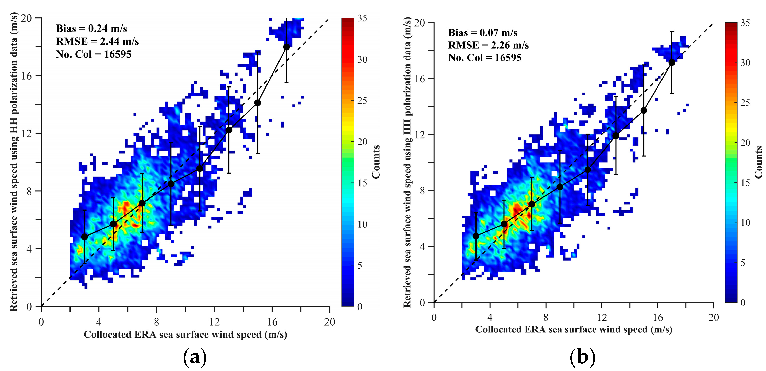
3.2. SSWS Retrieval from QPS HH Polarization Data

For GF-3 QPS HH polarization data, there are no well-developed and validated wind speed retrieval models currently available. The full polarization imaging capability of the GF-3 QPS mode provides a unique opportunity to study the polarization differences between VV and HH polarization data. Therefore, in this section, we study the dependence of the PR between QPS VV and HH polarization data on incidence angles, azimuth angles, and wind speeds. Based on these analyses, we determined an appropriate PR model to retrieve SSWS using the QPS HH polarization data.

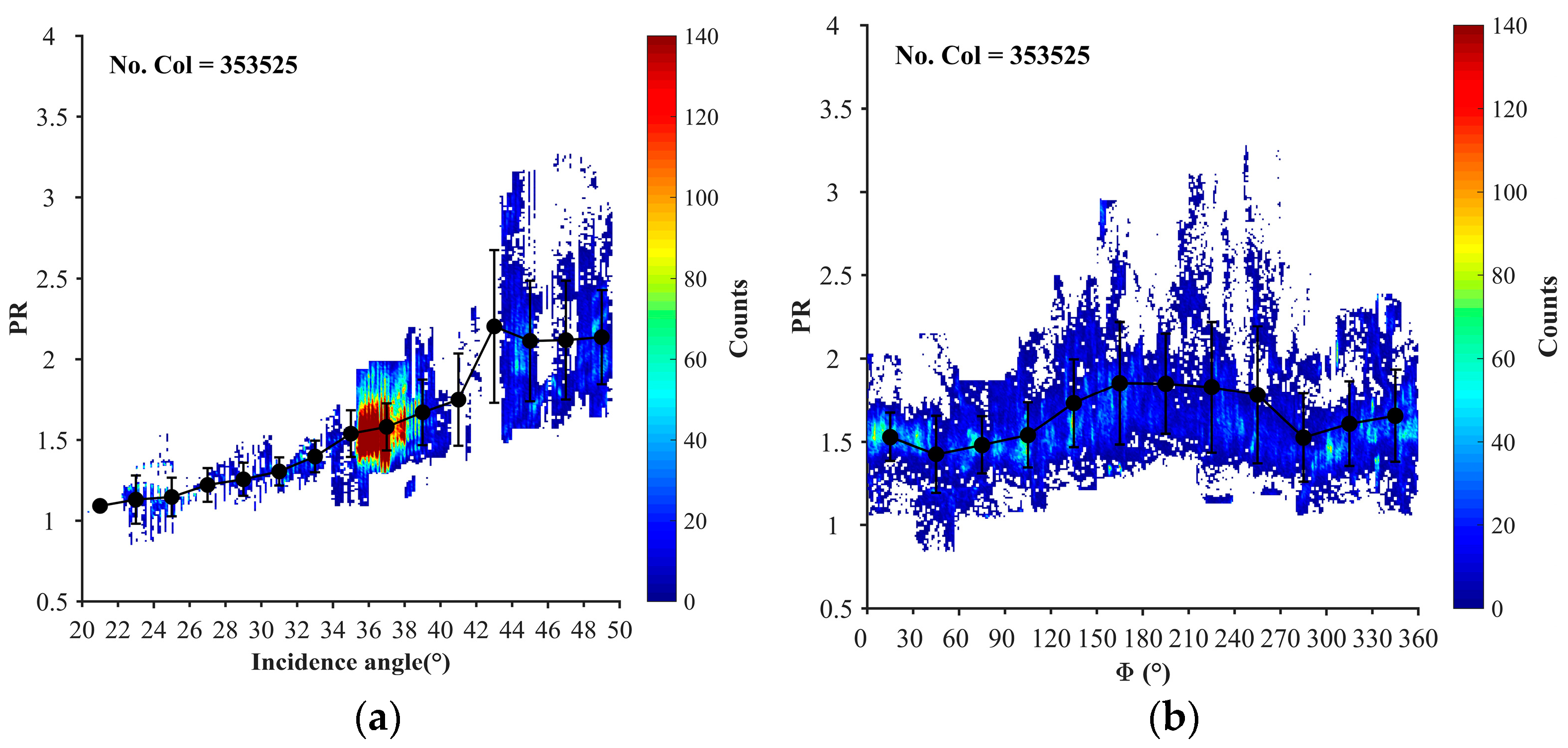
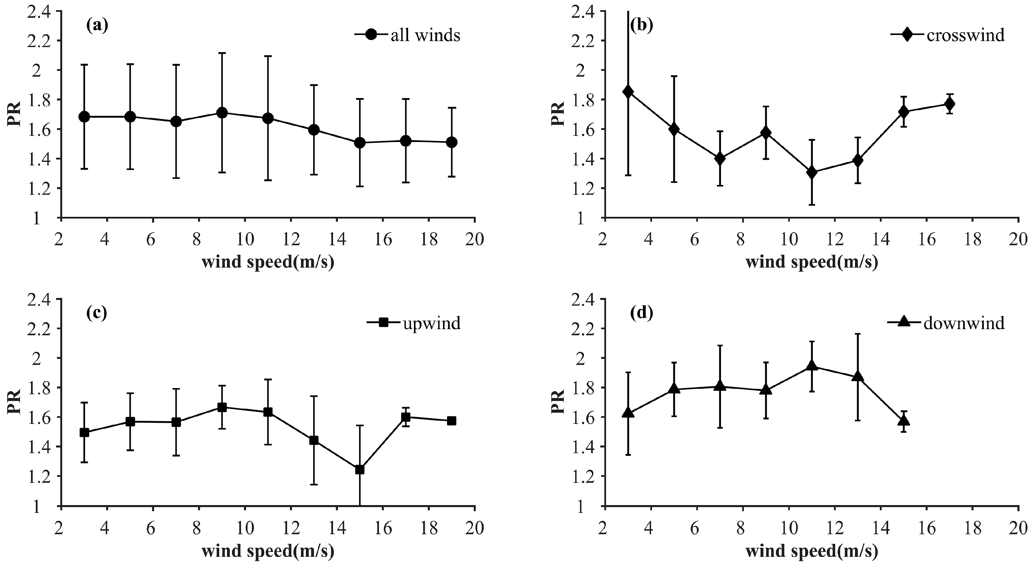
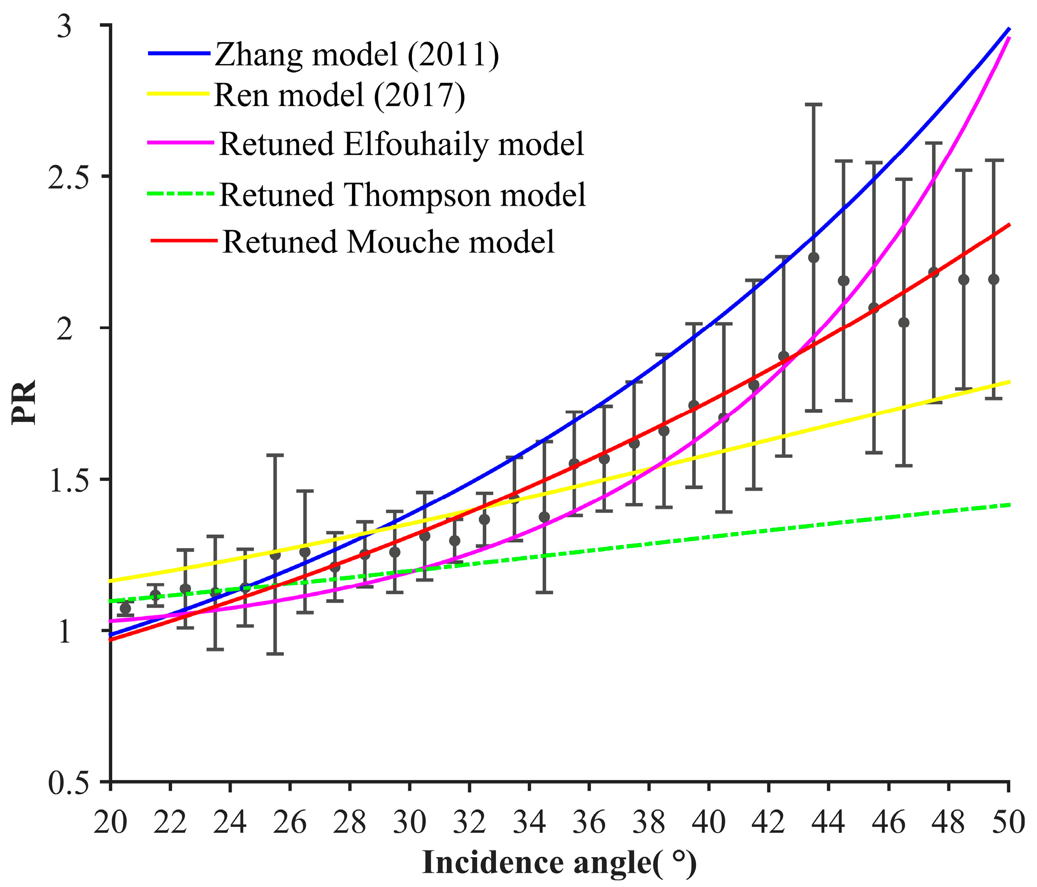
3.2.1. Development of the PR Model for GF-3 QPS HH Polarization Data

Following the usual notation, PR is defined as the ratio of VV NRCS to HH NRCS in a linear unit, given as:
PR = σ VV 0 / σ HH 0
Based on the measurements of GF-3 co-polarization sub-scenes and the collocated ERA-Interim reanalysis wind data, dependences of the PR on the incidence angle, the azimuth angle, and the wind speed were investigated and are shown in Figure 5a,b and Figure 6, respectively.
Figure 5a shows variations in the PR with an incidence angle, and error bars have been overlaid. In the diagram, the PR values present a firmly rising trend with an increasing incidence angle, which indicates that the PR has a significant dependence on the incidence angle. This is consistent with the results found by Ren et al. [44].
In Figure 5b, the dependence of the PR on the azimuth angle (Ф, which is defined in Equation (1)) is shown. The relationship between these two parameters presents a cosine-like variation. The maximum PR value is observed in the downwind direction (Ф = 180°), a secondary maximum value is close to the upwind direction (Ф = 0°), and the minimum is found approximately in the crosswind direction (Ф = 90° or 270°), which suggests that the PR values are dependent on the azimuth angle. This result is different from Ren’s result likely because their analysis only used the QPS data acquired at an SSWS of approximately 7 m/s.
To examine the dependence of the PR on SSWS, variations in the PR along with wind speed at different azimuth angles are studied, as shown in Figure 6. It is found that the mean PR values decrease slightly by approximately 0.2 (in terms of mean value) with increasing wind speed for all azimuth angles (Figure 6a). Fluctuations in the PR with wind speed in upwind (Figure 6c) and downwind (Figure 6d) directions are both weak (the steep drops in the upwind and downwind directions at 15 m/s are caused by the limited amount of data in that wind speed bin) while greater fluctuations are found in the crosswind direction. Overall, we did not find a clear dependence of the PR on SSWS.
In summary, the PR values of QPS VV and HH polarization data show clear dependence on the incidence and azimuth angles but a weak dependence on the SSWS.
Based on the analysis above, we consider fitting two types of PR models for the GF-3 QPS data. The first is the incidence angle-dependent PR model, referred to as the QPS-IA model, and the other is the incidence angle-dependent and azimuth angle-dependent model, referred to as the QPS-AA model.
To date, there are three generally accepted incidence angle-dependent PR models, i.e., the Elfouhaily model [22], the Thompson model [23], and the Mouche model [24], as shown in Equations (4)–(6), respectively. In these equations, α ,   β ,   A ,   B ,   and   C are constant coefficients that need to be tuned, and θ is the incidence angle.
PR ( θ ) = σ VV 0 σ HH 0 = ( 1 + 2   tan 2 θ ) 2 ( 1 + α   sin 2 θ ) 2
PR ( θ ) = σ VV 0 σ HH 0 = ( 1 + 2   tan 2 θ ) 2 ( 1 + β tan 2 θ ) 2
PR ( θ ) = A exp ( B θ ) + C
Using the iterative least squares estimation method, coefficients of the three above equations are fitted for the PR values, which are given in Table 3. Figure 7 shows the comparisons of the three fitted PR models with the true observations of the QPS data. In addition to the three refitted PR models, the other two PR models dependent on incidence angles, i.e., the Zhang model [25], which is derived from RS-2 data, and the Ren model [44], which is based on the GF-3 QPS data, are added to the comparison. The gray solid lines are the error bars of the PR values in the incidence angle bins. In the diagram, the Zhang model increases rapidly with the incidence angle, and its rate of increase is greater than those of the other models, especially when the incidence angle exceeds 34°. Furthermore, the discrepancy among the models increases with an increasing incidence angle. Therefore, the GF-3 PR values are generally lower than the RS-2 PR values at high incidence angles (>34°). On the other hand, the Ren model is too straight and far from the GF-3 QPS PR mean values (gray solid dots), which may be attributed to the QPS data concentrated at incidence angles of 35.5–37.5° degrees in their study. For the three retuned incidence angle-dependent PR models, the retuned Mouche model (red solid line) matches well with the mean PR value in each incidence angle bin and is regarded as the QPS-IA model, as given in Equation (7).
PR ( θ ) = 0.649 exp ( 0.0268 θ ) 0.14
Mouche et al. [24] also proposed another PR model that is dependent on both the incidence angle and the azimuth angle, as shown in Equation (8). For each azimuth angle, the dependence of PR on the incidence angle follows an exponential relationship, as shown in Equation (9). The coefficients C 0 ,   C 1 ,   and   C 2 in Equation (8) correspond to the upwind, crosswind, and downwind directions (Equations (10)–(12)), respectively. This model is retuned for the QPS data and is referred to as the QPS-AA model in the following. Its coefficients are listed in Table 4.
PR ( θ , Φ ) = C 0 ( θ ) + C 1 ( θ ) cos Φ + C 2 ( θ ) cos 2 Φ
PR Φ ( θ ) = A Φ exp ( B Φ θ ) + C Φ
C 0 ( θ ) = ( PR 0 ( θ ) + PR π ( θ ) + 2 PR π / 2 ( θ ) ) / 4
C 1 ( θ ) = ( PR 0 ( θ ) PR π ( θ ) ) / 2
C 2 ( θ ) = ( PR 0 ( θ ) + PR π ( θ ) 2 PR π / 2 ( θ ) ) / 4

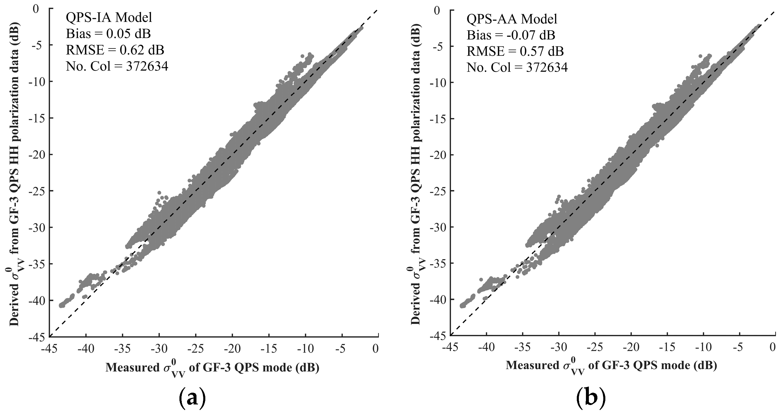
3.2.2. SSWS Retrieval from the QPS HH Polarization Data

Prior to SSWS retrieval using the QPS HH polarization data, we first compared the SAR observed σ VV 0 values with those converted using the two refitted PR models presented above, which are shown in Figure 8a,b, respectively. Generally, the converted σ VV 0 by the two PR models are in good agreement with the observations, which further proves the effectiveness of the two PR models. The QPS-AA model has slightly better performance (with an RMSE of 0.57 dB) than the QPS-IA model (with an RMSE of 0.62 dB).
Then, the two PR models combined with CMOD5.N are used to retrieve SSWS from the QPS HH polarization data and are compared with the ERA-Interim reanalysis model results, as shown in Figure 9a,b. Error bars are overlaid on the scatter plots. In terms of both bias and RMSE, the QPS-AA model yields better SSWS retrieval than the QPS-IA model. Similar to Figure 4, a majority of the data points are concentrated between 2 m/s and 8 m/s. In this range, the retrievals using the QPS-AA model are higher than the ERA-Interim reanalysis wind speed by 0.52 m/s on average. For wind speeds greater than 7 m/s, the SSWS derived from HH polarization data also tends to be lower than the ERA-Interim model results. For high wind speeds (>12 m/s), the amount of data is insufficient to draw reasonable conclusions.

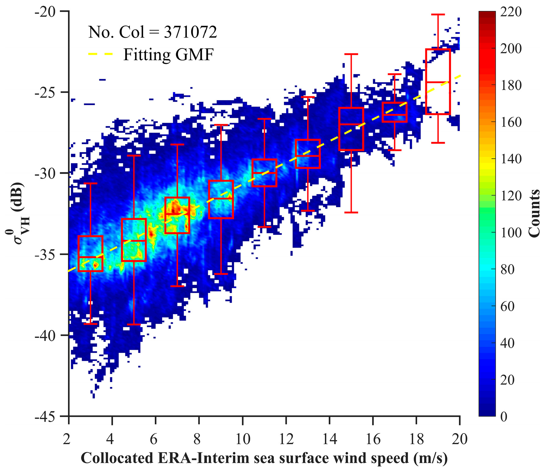
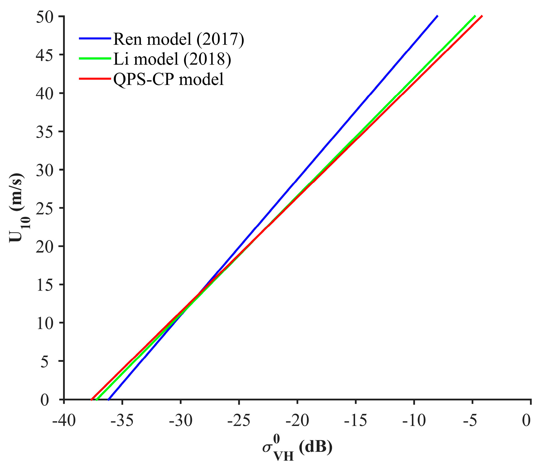
3.3. SSWS Retrieval from QPS VH Polarization Data

Following the analysis of GF-3 QPS co-polarization data, the possibility of deriving SSWS from cross-polarization data is explored. Based on the principle of reciprocity, the VH and HV polarization data are highly similar. In view of many previous studies on SAR SSWS retrieval by polarization data, we choose the VH polarization as the representative cross-polarization to conduct the analysis.
Figure 10 shows the scatter density map of σ VH 0 and the collocated ERA-Interim U 10 , on which box-whisker plots have been overlaid. The lower limits of the box-whisker plots in the low wind speed (approximately 4–5 m/s) suggest that the noise equivalent sigma zero (NESZ) of the GF-3 QPS cross-polarization data is approximately −38 dB to −39 dB. In the diagram, the σ VH 0 median values present a clear linear increasing trend with increasing SSWS. Therefore, a linear function related to the QPS cross-polarization NRCS σ VH 0 (in dB) with the SSWS is derived, as indicated by the yellow dotted line in Figure 10. The linear function used to derive wind speed is called the QPS-CP model afterward and is given in Equation (13).
σ VH 0 = 0.6683 U 10 37.3732
Figure 11 suggests that the performance of the QPS-CP model is very similar to that of our previous result in Reference [41], which are both tuned using the ERA-Interim reanalysis model wind. On the other hand, the QPS-CP model derived from a greater number of collocated samples agrees well with the one proposed by Li et al. [41], which indicates the stability of the statistical analysis in both analyses. The discrepancy between the QPS-CP model and the Ren et al. [44] result is distinct. For SSWSs less than 13 m/s, the QPS-CP model yields higher estimates than the Ren model. For greater SSWSs, the slope of Ren’s linear function is higher than that of the QPS-CP model, which results in higher estimates of the SSWS in severe wind situations. The discrepancies between the two models can be attributed to two reasons. On the one hand, the QPS-CP model was tuned based on the ERA-Interim reanalysis wind model results, while the Ren model is based on the GFS wind data. On the other hand, different amounts of QPS data may also lead to different tuning results of the linear functions.
Figure 12 shows the comparison between the retrieved wind speed using the QPS-CP model and the collocated independent WindSat wind data within a 95% confidence interval. The data with wind speeds less than 2 m/s are discarded from the analysis. The different colors indicate the incidence angles of the QPS data. The comparison yields an RMSE and a bias of 2.02 m/s and 0.1 m/s, respectively. The mean values (black solid dots) of each 2 m/s bin in the diagram show good agreement between the SAR retrieval and WindSat data for SSWSs ranging from 4 m/s to 18 m/s. Notably, however, the retrieved wind speed for the QPS data acquired at incidence angles of less than approximately 27° (11.86%) are mostly larger than the WindSat results, with a high bias of 2.35 m/s and an RMSE of 2.95 m/s. However, the trend in the data acquired at incidence angles greater than approximately 47° (10.39%) is the opposite. The retrieved wind speeds are lower than the WindSat SSWS results, with a bias of −1.07 m/s and an RMSE of 1.70 m/s. The bias and RMSE for data acquired at incidence angles ranging from 27° to 47° are −0.05 m/s and 1.93 m/s, respectively, which are consistent with the results in our previous study [41]. There are two plausible explanations for these discrepancies. On the one hand, the discrepancies indicate that the relation between the QPS cross-polarization NRCS and the SSWS is not fully SSWS dependent and that the incidence angle may also contribute. On the other hand, the radiometric calibration of the QPS cross-polarization data with steep and shallow incidence angles requires particular attention.
As mentioned in the Introduction, SAR cross-polarization data have been extensively used to derive SSWSs for severe tropical storms. However, the above analysis is dedicated to GF-3 QPS data with swath widths of approximately 25–40 km, which is not very useful for typhoon or hurricane observations. However, the difficulty is that the amount of data acquired from GF-3 wide swath data is not sufficient to conduct a similar analysis as that presented above. We, therefore, attempt to directly apply the derived QPS-CP model to the GF-3 Wide ScanSAR (WSC) data. A GF-3 WSC mode data for the typhoon SOULIK was acquired on 19 August 2018, at 8:46 UTC. The data has a swath width of 500 km and a pixel size of 100 m. The incidence angle ranges from 14° to 41°. We applied the QPS-CP model to this WSC data in VH polarization and derived the SSWSs, as shown in Figure 13. The colored arrows represent the GFS SSW data at 9:00 UTC on 19 August. The SAR-derived SSWSs show some agreements with the GFS wind speeds. The averaged GFS wind speed around the typhoon wall is 27.5 m/s, which is slightly higher than the highest SAR-derived SSWS of 24.2 m/s. This example indicates the feasibility of using the QPS-CP model for high SSWS retrieval from GF-3 SAR data. However, the GFS peak wind is 38.76 m/s, whereas the SAR-derived peak wind is only 25.88 m/s. The current QPS-CP model is tuned using the ERA-Interims data while all the wind speeds of collocation samples are less than 20 m/s. It is desired to operate the sensor to acquire data over high wind regions to retune the relation between the NRCS of VH polarization data and SSWS. On the other hand, it seems that the NRCS of VH polarization in this case has weak dependence on incidence angles since the derived SSWS does not transition smoothly from beam to beam. While more ScanSAR data are being acquired, this issue requires further investigation.

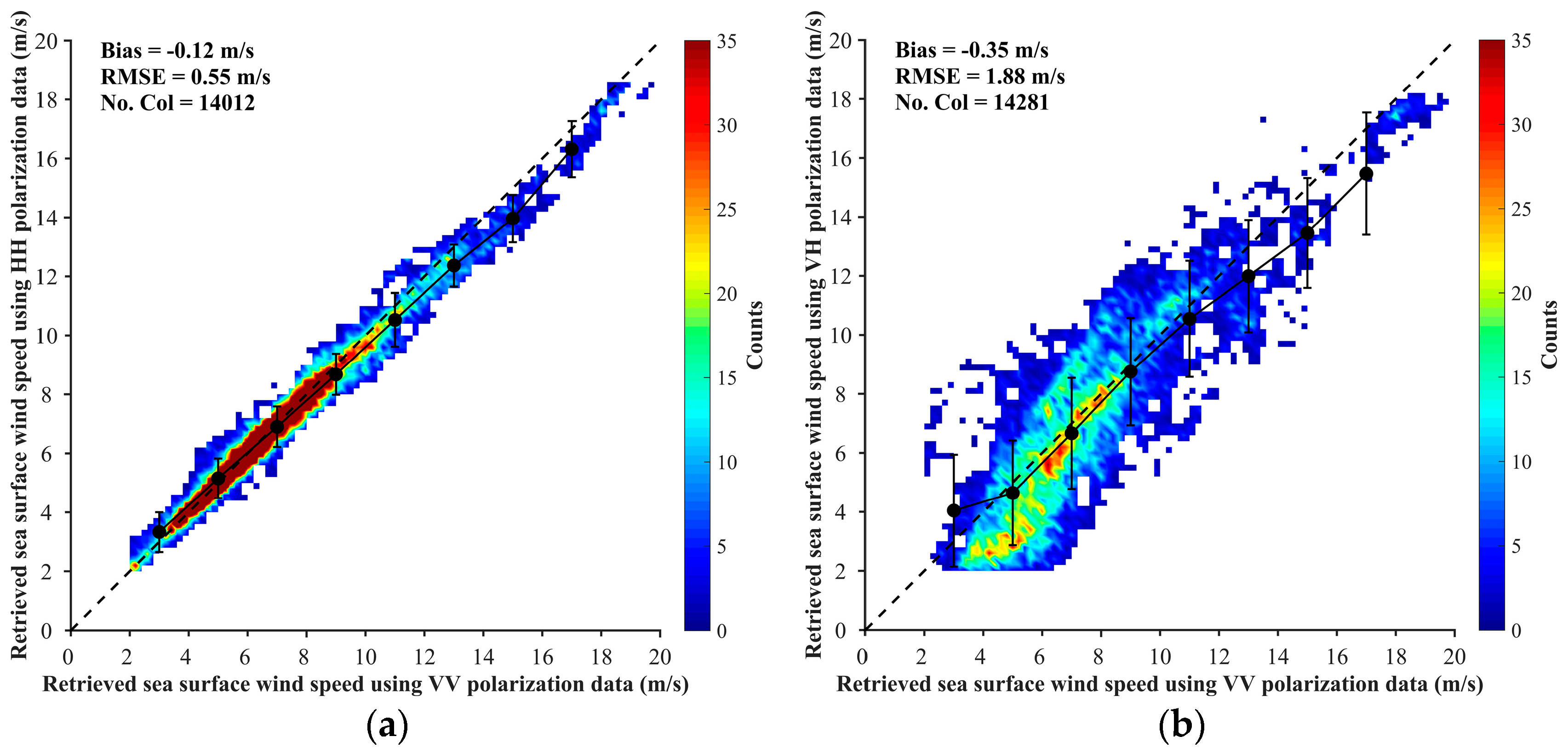
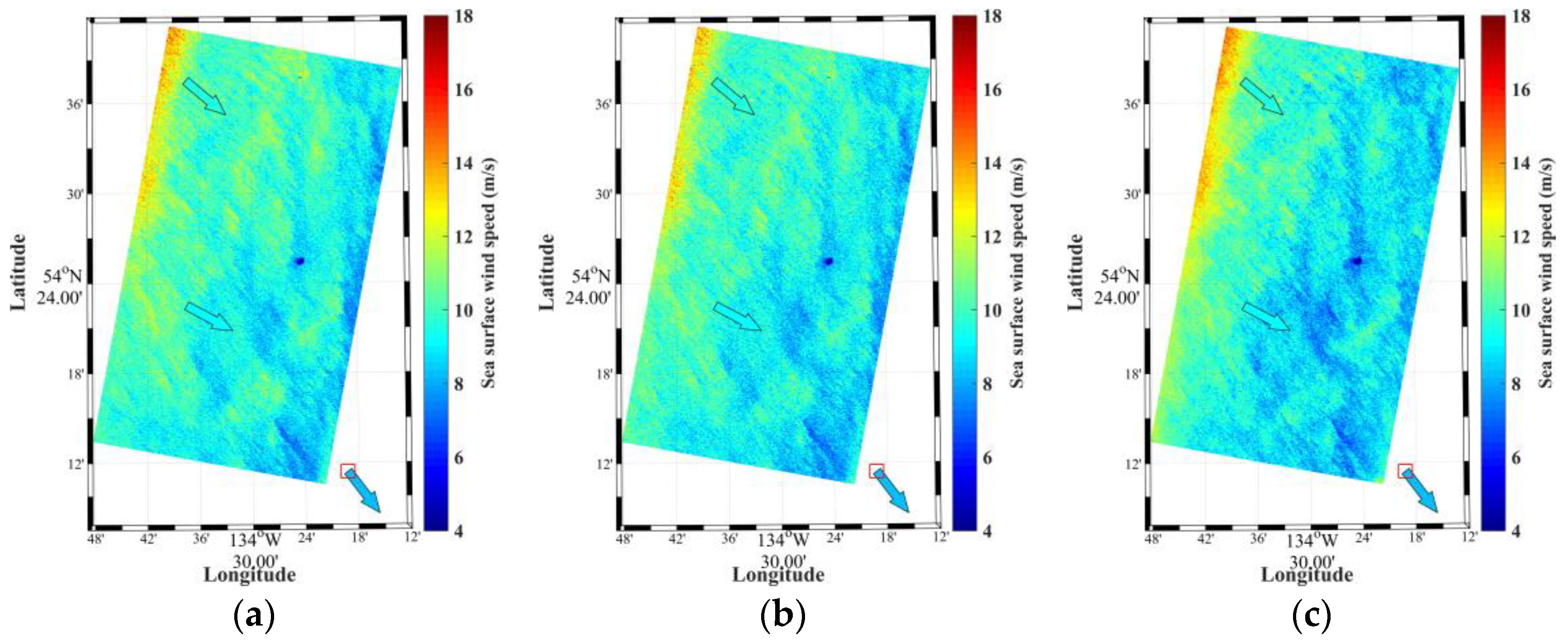
3.4. Intercomparison of SSWS Retrieval from VV, HH, and VH Polarizations of GF-3 QPS Data

Figure 14a,b are comparisons of the retrieved SSWSs based on the VV, HH, and VH polarizations of the GF-3 QPS data. The QPS-AA model and QPS-CP model are used for retrieving the SSWSs from the HH and VH polarization data, respectively. Figure 14a suggests a good SSWS retrieval consistency between the HH and VV polarization data with a bias of −0.12 m/s and an RMSE of 0.55 m/s.
A comparison of retrievals from the VV and VH data is shown in Figure 14b, which yields a bias of −0.35 m/s and an RMSE of 1.88 m/s. For wind speeds between 4 m/s and 12 m/s, for which there is abundant data, the retrievals from the VH and VV polarizations are in good agreement. However, as the wind speed increases, the VH polarization-derived SSWS tends to be lower than VV polarization-derived SSWS.
In addition, an example of wind speed retrieval from three different polarizations of the QPS mode data is shown in Figure 15a–c. The SAR data were acquired at 15:15 UTC on 25 May 2017. The overlaid arrows indicate the WindSat-derived SSW at 15:48 UTC on the same day. The external reference wind directions used for SSWS retrieval from VV and HH polarization data are the collocated ERA-Interim reanalysis model wind directions. The SSWSs of the three polarizations are generally in good agreement especially the VV and HH polarization results. The average wind speed difference is 0.19 m/s between the VV and HH polarizations and 0.3 m/s between the VV and VH polarizations, which are consistent with the overall biases in Figure 14a,b. These results also agree well with the WindSat wind speeds. The nearby Canadian buoy (46205) is in the southeast of the GF-3 SAR image and is marked by a square in the three plots. The buoy measurement of wind speed (15:38 UTC) at 5 m height is converted at 10 m height assuming neutral wind, which results in a value of 8.2 m/s. The buoy wind direction is 323°. The SAR-derived SSWSs closest to the buoy location are 8.2 m/s, 8.0 m/s, and 8.1 m/s (based on a 2 km by 2 km subscene) for the three polarizations.

4. Conclusions

Accurate radiometric calibration is a prerequisite for retrieving exact SSWSs from spaceborne SAR data. Considering that the general accuracy of spaceborne SAR retrieved SSWS data is less than 0.5 m/s, the radiometric calibration accuracy requirement of SAR data is estimated by CMOD5.N. The result shows that, to achieve a bias of less than 0.5 m/s for SSWS retrieval using CMOD5.N, 1.3 dB is the lowest calibration requirement for any C-band SAR. The calibration accuracy verification of QPS mode VV polarization is conducted by investigating the difference (∆σ) between the measured VV NRCS and the simulated VV NRCS, which are calculated based on CMOD5.N using ERA-Interim reanalysis SSWS data. The mean values of ∆σ in each 1° incidence angle bin for incidence angles between approximately 27° and 49° are within ±1.3 dB, which meet the requirements of the wind speed retrieval accuracy with an absolute bias of less than 0.5 m/s. The average mean value of ∆σ in each 1° incidence angle bin is 0.53 dB, which is less than the absolute radiometric error (less than 1.5 dB) for all modes of GF-3 [37] and is also comparable with the absolute calibration accuracy of 0.21 dB for image mode data from ASAR [50], 0.15 dB for RS-2 in all modes [51], and 0.39 dB for stripmap mode data from Sentinel-1 [52]. Therefore, the overall calibration accuracy of GF-3 QPS mode VV polarization is not poor. However, the GF-3 QPS VV polarization data show a high standard deviation (approximately 2.0–2.5 dB) in the absolute calibration factor, which is much higher than those of other spaceborne SAR data. In comparison, the ASAR image mode data have a standard deviation of 0.58 dB [50], and the Sentinel-1 stripmap data have a standard deviation of 0.25–0.45 dB [52,53]. Although our study on this issue is based on simulation experiments, which are not as precise as the radiometric calibration studies using ground truth measurements (e.g., corner reflectors and transponders), our work at least points out the radiometric calibration problems of the GF-3 QPS data that need to be addressed when using these data to retrieve sea surface dynamic parameters.
The comparison of retrieved wind speed data from VV polarization data with ERA-Interim reanalysis wind speed data shows general agreement, with a bias of 0.18 m/s and an RMSE of 2.36 m/s. Because the standard deviations of the radiometric calibration factors of the QPS VV polarization data are rather high, it is understandable why the SSWS comparison yields a high RMSE value. The PR values of the GF-3 QPS data show a clear dependence on the incidence and azimuth angles but weak dependence on the SSWS. Thus, two PR models, an incidence angle-dependent model (the QPS-IA model) and an incidence angle- and azimuth angle-dependent model (the QPS-AA model), have been retuned. A comparison of the converted NRCS of VV polarization with the measured values using the two PR models suggests that the QPS-AA model performs slightly better than the QPS-IA model. The retrieved SSWS from the QPS HH polarization data using the QPS-AA model has very good agreement with that from the QPS VV polarization data, with a bias of −0.12 m/s and an RMSE of 0.55 m/s. We, therefore, recommend the QPS-AA model, which considers both incidence angle and azimuth angle dependence, as the PR model for SSW retrieval from QPS HH polarization data.
The NRCS of the QPS VH polarization shows a linear relationship with increasing SSWS. Therefore, a linear wind speed retrieval function called QPS-CP was fitted. The QPS-CP proposed here has a very similar performance as that proposed in our previous study [41], although the amount of data is different. This finding suggests that the current acquisitions of QPS cross-polarization data are sufficient to derive a stable linear function to derive SSWS directly. However, one should note that any empirical function such as the one proposed here is strongly related to the reference values. In this study, we used the ERA-Interim wind speed as reference of sea surface wind speed. Currently, a higher spatial (31 km) and temporal (hourly) resolution reanalysis model, ERA-5, is also available. On the other hand, along with more acquisitions of the GF-3 SAR data over buoys, developing a more accurate QPS-CP model should be performed. Second, the application of the QPS-CP model to SSWS retrieval shows incidence angle discrepancy. The retrieved SSWSs are consistent with the WindSat results when incidence angles range from 27° to 47°, with a small bias of −0.05 m/s. When incidence angles are less than 27° or greater than 47°, the derived SSWSs are larger or lower than the WindSat measurements, respectively, with absolute biases greater than 1 m/s. However, it is still difficult to determine whether the incidence angle should be another factor for QPS-CP model optimization or the QPS data at low and high incidence angles have some radiometric calibration problems because wind speed retrievals from VV polarization data have been found to be abnormal in this range of incidence angles.
Thus far, based on this study and the recent study of Li et al. [41], we can conclude that SSWS retrieval from different polarizations of the current GF-3 QPS data has accuracy of a bias of less than 0.3 m/s and an RMSE of 2.0 ± 0.2 m/s depending on various comparison datasets. Further improving the accuracy of SSWS retrieval from GF-3 QPS data will depend on dedicated efforts involving radiometric calibration of different beams and polarization channels.

Author Contributions

Conceptualization, X.-M.L.; Formal analysis, T.Z.; Funding acquisition, X.-M.L.; Investigation, T.Z., X.-M.L. and Y.S.; Methodology, T.Z., X.-M.L., Q.F., Y.R. and Y.S.; Project administration, X.-M.L.; Resources, X.-M.L.; Supervision, X.-M.L.; Writing – original draft, T.Z.; Writing – review & editing, X.-M.L., Q.F., Y.R. and Y.S.

Funding

The National Key Research and Development Program of China (2016YFC1401001, 2018YFC1407100) and the National Natural Science Foundation of China (grant no.41471309) funded this research.

Acknowledgments

The authors thank the National Satellite Ocean Application Service for providing GF-3 SAR data. The GF-3 data availability is a concern for scientific communication. So far, as we know that some international scholars have accessed GF-3 SAR data via the ESA-MOST “Dragon” program (http://dragon4.esa.int/page_home.php). We would also like to acknowledge the ECMWF, the Fisheries and Oceans Canada and Remote Sensing Systems for offering wind field dataset. The ERA-Interim reanalysis wind data are free available via https://apps.ecmwf.int/datasets/data/interim-full-daily/levtype=sfc/. The GFS model data are accessed from NOAA via https://www.ncdc.noaa.gov/data-access/model-data/model-datasets/global-forcast-system-gfs. Website of downloading WindSat data is http://www.remss.com/missions/windsat/. The wind data of buoy number C46205 are downloaded from http://www.dfo-mpo.gc.ca/index-eng.htm.

Conflicts of Interest

The authors declare no conflict of interest.

References

  1. Pond, S.; Pickard, G.L. Currents with Friction; Wind-driven Circulation. In Introductory Dynamical Oceanography, 2nd ed.; Pond, S., Pickard, G.L., Eds.; Elsevier Publishing: Amsterdam, The Netherlands, 2013; pp. 100–162. [Google Scholar]
  2. Mattie, M.G.; Lichy, D.E.; Beal, R.C. Seasat detection of waves, currents and inlet discharge. Int. J. Remote Sens. 1980, 1, 377–398. [Google Scholar] [CrossRef]
  3. Vesecky, J.F.; Stewart, R.H. The observation of ocean surface phenomena using imagery from the SEASAT synthetic aperture radar: An assessment. J. Geophys. Res.-Oceans 1982, 87, 3397–3430. [Google Scholar] [CrossRef]
  4. Gerling, T.W. Structure of the surface wind field from the Seasat SAR. J. Geophys. Res. 1986, 91, 2308–2320. [Google Scholar] [CrossRef]
  5. Lehner, S.; Horstmann, J.; Koch, W.; Rosenthal, W. Mesoscale wind measurements using recalibrated ERS SAR images. J. Geophys. Res.-Oceans 1998, 103, 7847–7856. [Google Scholar] [CrossRef] [Green Version]
  6. Koch, W. Directional analysis of SAR images aiming at wind direction. IEEE Trans. Geosci. Remote Sens. 2004, 42, 702–710. [Google Scholar] [CrossRef]
  7. Wang, Y.R.; Li, X.M. Derivation of sea surface wind directions from TerraSAR-X data using the Local Gradient method. Remote Sens. 2016, 8, 53. [Google Scholar] [CrossRef]
  8. Levy, G. Boundary layer roll statistics from SAR. Geophys. Res. Lett. 2001, 28, 1993–1995. [Google Scholar] [CrossRef] [Green Version]
  9. Zhao, Y.; Li, X.M.; Sha, J. Sea surface wind streaks in spaceborne synthetic aperture radar imagery. J. Geophys. Res.-Oceans 2016, 121, 6731–6741. [Google Scholar] [CrossRef]
  10. Holt, B. SAR imaging of the ocean surface. In Synthetic Aperture Radar Marine User’s Manual; Apel, J.R., Jackson, C.R., Eds.; U.S. Department of Commerce: Washington, DC, USA, 2004; pp. 25–80. [Google Scholar]
  11. Stoffelen, A.; Anderson, D. Scatterometer data interpretation: Derivation of the transfer function CMOD4. J. Geophys. Res. 1997, 102, 5767–5780. [Google Scholar] [CrossRef]
  12. Quilfen, Y.; Chapron, B.; Elfouhaily, T.; Katsaros, K.; Tournadre, J. Observation of tropical cyclones by high-resolution scatterometry. J. Geophys. Res. 1998, 103, 7767–7786. [Google Scholar] [CrossRef] [Green Version]
  13. Hersbach, H.; Stoffelen, A.; De Haan, S. An improved C-band scatterometer ocean geophysical model function: CMOD5. J. Geophys. Res. 2007, 112, C03006. [Google Scholar] [CrossRef]
  14. Hersbach, H. Comparison of C-Band scatterometer CMOD5.N equivalent neutral winds with ECMWF. J. Atmos. Oceanic Technol. 2010, 27, 721–736. [Google Scholar] [CrossRef]
  15. Elyouncha, A.; Neyt, X.; Stoffelen, A.; Verspeek, J. Assessment of the corrected CMOD6 GMF using scatterometer data. Remote Sens. Ocean Sea Ice Coast. Waters Large Water Reg. 2015, 9638. [Google Scholar] [CrossRef]
  16. Stoffelen, A.; Verspeek, J.; Vogelzang, J.; Verhoef, A. The CMOD7 Geophysical Model Function for ASCAT and ERS Wind Retrievals. IEEE J. Sel. Top. Appl. Earth Obs. Remote Sens. 2017, 10, 2123–2134. [Google Scholar] [CrossRef]
  17. Ren, Y.Z.; Lehner, S.; Brusch, S.; Li, X.M.; He, M.X. An algorithm for the retrieval of sea surface wind fields using X-band TerraSAR-X data. Int. J. Remote Sens. 2012, 33, 7310–7336. [Google Scholar] [CrossRef]
  18. Li, X.M.; Lehner, S. Algorithm for sea surface wind retrieval from TerraSAR-X and TanDEM-X data. IEEE Trans. Geosci. Remote Sens. 2014, 52, 2928–2939. [Google Scholar] [CrossRef]
  19. Isoguchi, O.; Shimada, M. An L-Band Ocean Geophysical Model Function Derived From PALSAR. IEEE Trans. Geosci. Remote Sens. 2009, 47, 1925–1936. [Google Scholar] [CrossRef]
  20. Phillips, O.M. Spectral and equilibrium properties of the equilibrium range in the wind-generated gravity waves. J. Fluid Mech. 1985, 156, 505–531. [Google Scholar] [CrossRef]
  21. Monaldo, F.M.; Thompson, D.R.; Pichel, W.G.; Clemente, P. A Systematic Comparison of Quikscat and SAR Ocean Surface Wind Speeds. IEEE Trans. Geosci. Remote Sens. 2004, 42, 283–291. [Google Scholar] [CrossRef]
  22. Elfouhaily, T. Physical Modeling of Electromagnetic Backscatter from the Ocean Surface; Application to Retrieval of Wind Fields and Wind Stress by Remote Sensing of the Marine Atmospheric Boundary Layer. Ph.D. Thesis, Univ. Paris VII, Paris, France, 1996. [Google Scholar]
  23. Thompson, D.R.; Elfouhaily, T.M.; Chapron, B. Polarization ratio for microwave backscattering from the ocean surface at low to moderate incidence angles. In Proceedings of the IEEE International Geoscience and Remote Sensing (IGARSS), Seattle, WA, USA, 6–10 July 1998; pp. 1671–1673. [Google Scholar]
  24. Mouche, A.; Hauser, D.; Daloze, J.F.; Guerin, C. Dual-polarization measurements at C-band over the ocean: Results from airborne radar observations and comparison with ENVISAT ASAR data. IEEE Trans. Geosci. Remote Sens. 2005, 43, 753–769. [Google Scholar] [CrossRef]
  25. Zhang, B.; Perrie, W.; He, Y.J. Wind speed retrieval from RADARSAT-2 quad-polarization images using a new polarization ratio model. J. Geophys. Res.-Oceans 2011, 116, C08008. [Google Scholar] [CrossRef]
  26. Yang, X.F.; Li, X.F.; Pichel, W.G.; Li, Z.W. Comparison of Ocean Surface Winds from ENVISAT ASAR, MetOp ASCAT Scatterometer, Buoy Measurements, and NOGAPS Model. IEEE Trans. Geosci. Remote Sens. 2011, 49, 4743–4750. [Google Scholar] [CrossRef]
  27. Komarov, A.S.; Zabeline, V.; Barber, D.G. Ocean surface wind speed retrieval from C-band SAR images without wind direction input. IEEE Trans. Geosci. Remote Sens. 2014, 52, 980–990. [Google Scholar] [CrossRef]
  28. Stopa, J.E.; Mouche, A.A.; Chapron, B.; Collard, F. Sea State Impacts on Wind Speed Retrievals From C-Band Radars. IEEE J. Sel. Top. Appl. Earth Observ. Remote Sens. 2017, 10, 2147–2155. [Google Scholar] [CrossRef]
  29. Reppucci, A.; Lehner, S.; Schulz-Stellenfleth, J. Tropical Cyclone Parameters Derived from Synthetic Aperture Radar (SAR) Images. In Proceedings of the 2006 IEEE International Symposium on Geoscience and Remote Sensing, Denver, CO, USA, 31 July–4 August 2006; pp. 2220–2223. [Google Scholar] [CrossRef]
  30. Vachon, P.W.; Wolfe, J. C-Band Cross-Polarization Wind Speed Retrieval. IEEE Geosci. Remote Sens. Lett. 2011, 8, 456–459. [Google Scholar] [CrossRef]
  31. Hwang, P.A.; Zhang, B.; Toporkov, J.V.; Perrie, W. Comparison of composite Bragg theory and quad-polarization radar backscatter from RADARSAT-2: With applications to wave breaking and high wind retrieval. J. Geophys. Res. Oceans 2010, 115, C08019. [Google Scholar] [CrossRef]
  32. Zhang, B.; Perrie, W. Cross-Polarized Synthetic Aperture Radar: A New Potential Measurement Technique for Hurricanes. Bull. Am. Meteorol. Soc. 2012, 93, 531–541. [Google Scholar] [CrossRef] [Green Version]
  33. Van Zadelhoff, G.J.; Stoffelen, A.; Vachon, P.W.; Wolfe, J.; Horstmann, J.; Belmonte-Rivas, M. Retrieving hurricane wind speeds using cross-polarization C-band measurements. Atmos. Meas. Tech. 2014, 7, 437–449. [Google Scholar] [CrossRef] [Green Version]
  34. Horstmann, J.; Falchetti, S.; Wackerman, C.; Maresca, S.; Caruso, M.J.; Graber, H.C. Tropical Cyclone Winds Retrieved from C-Band Cross-Polarized Synthetic Aperture Radar. IEEE Trans. Geosci. Remote Sens. 2015, 53, 2887–2898. [Google Scholar] [CrossRef]
  35. Hwang, P.A.; Perrie, W.; Zhang, B. Cross-Polarization Radar Backscattering from the Ocean Surface and Its Dependence on Wind Velocity. IEEE Geosci. Remote Sens. Lett. 2014, 11, 2188–2192. [Google Scholar] [CrossRef]
  36. Hwang, P.A.; Stoffelen, A.; Zadelhoff, G.J.V.; Perrie, W.; Zhang, B.; Li, H.; Shen, H. Cross-polarization geophysical model function for C-band radar backscattering from the ocean surface and wind speed retrieval. J. Geophys. Res. Oceans 2015, 120, 893–909. [Google Scholar] [CrossRef] [Green Version]
  37. Sun, J.; Yu, W.; Deng, Y. The SAR Payload Design and Performance for the GF-3 Mission. Sensors 2017, 17, 2419. [Google Scholar] [CrossRef] [PubMed]
  38. Wang, T.; Zhang, G.; Yu, L.; Zhao, R.; Deng, M.; Xu, K. Multi-Mode GF-3 Satellite Image Geometric Accuracy Verification Using the RPC Model. Sensors 2017, 17, 2005. [Google Scholar] [CrossRef] [PubMed]
  39. Chang, Y.; Li, P.; Yang, J.; Zhao, J.; Zhao, L.; Shi, L. Polarimetric Calibration and Quality Assessment of the GF-3 Satellite Images. Sensors 2018, 18, 403. [Google Scholar] [CrossRef] [PubMed]
  40. Zhang, Q. System design and key technologies of the GF-3 satellite. Acta Geod. Cartogr. Sin. 2017, 46, 269–277. [Google Scholar] [CrossRef]
  41. Li, X.M.; Zhang, T.; Huang, B.; Jia, T. Capabilities of Chinese Gaofen-3 Synthetic Aperture Radar in Selected Topics for Coastal and Ocean Observations. Remote Sens. 2018, 10, 1929. [Google Scholar] [CrossRef]
  42. Wang, H.; Yang, J.; Mouche, A.; Shao, W.; Zhu, J.; Ren, L.; Xie, C. GF-3 SAR Ocean Wind Retrieval: The First View and Preliminary Assessment. Remote Sens. 2017, 9, 694. [Google Scholar] [CrossRef]
  43. Shao, W.; Sheng, Y.; Sun, J. Preliminary Assessment of Wind and Wave Retrieval from Chinese Gaofen-3 SAR Imagery. Sensors 2017, 17, 1705. [Google Scholar] [CrossRef]
  44. Ren, L.; Yang, J.; Mouche, A.; Wang, H.; Wang, J.; Zheng, G.; Zhang, H. Preliminary Analysis of Chinese GF-3 SAR Quad-Polarization Measurements to Extract Winds in Each Polarization. Remote Sens. 2017, 9, 1215. [Google Scholar] [CrossRef]
  45. Horstmann, J.; Koch, W.; Lehner, S.; Tonboe, R. Wind retrieval over the ocean using synthetic aperture radar with C-band HH polarization. IEEE Trans. Geosci. Remote Sens. 2000, 38, 2122–2131. [Google Scholar] [CrossRef]
  46. Schulz-Stellenfleth, J.; Lehner, S. Measurement of 2-D sea surface elevation fields using complex synthetic aperture radar data. IEEE Trans. Geosci. Remote Sens. 2004, 42, 1149–1160. [Google Scholar] [CrossRef]
  47. Gaiser, P.W.; Germain, K.M.S.; Twarog, E.M.; Poe, G.A.; Purdy, W.; Richardson, D.; Grossman, W.; Jones, W.L.; Spencer, D.; Golba, G.; et al. The WindSat spaceborne polarimetric microwave radiometer: Sensor description and early orbit performance. IEEE Trans. Geosci. Remote Sens. 2004, 42, 2347–2361. [Google Scholar] [CrossRef]
  48. Hilburn, K.A.; Meissner, T.; Wentz, F.J.; Brown, S.T. Ocean Vector Winds from WindSat Two-Look Polarimetric Radiances. IEEE Trans. Geosci. Remote Sens. 2016, 54, 918–931. [Google Scholar] [CrossRef]
  49. Portabella, M.; Stoffelen, A. On Scatterometer Ocean Stress. J. Atmos. Ocean. Technol. 2009, 26, 2. [Google Scholar] [CrossRef]
  50. Miranda, N.; Rosich, B.; Meadows, P.J.; Haria, K.; Small, D.; Schubert, A.; Lavalle, M.; Collard, F.; Johnsen, H.; Guarnieri, A.M. The EnviSAT ASAR Mission: A Look Back At 10 Years of Operation; European Space Agency Special Publication: Paris, France, 2013. [Google Scholar]
  51. Williams, D.; LeDantec, P.; Chabot, M.; Hillman, A.; James, K.; Caves, R.; Thompson, A.; Vigneron, C.; Wu, Y. RADARSAT-2 Image Quality and Calibration Update. In Proceedings of the 10th European Conference on Synthetic Aperture Radar (EUSAR), Berlin, Germany, 3–5 June 2014; pp. 1–4. [Google Scholar]
  52. Schwerdt, M.; Schmidt, K.; Ramon, N.T.; Alfonzo, G.C.; Döring, B.J.; Zink, M.; Prats-Iraola, P. Independent Verification of the Sentinel-1A System Calibration. IEEE J. Sel. Top. Appl. Earth Observ. 2016, 9, 994–1007. [Google Scholar] [CrossRef]
  53. Schwerdt, M.; Schmidt, K.; Tous Ramon, N.; Klenk, P.; Yague-Martinez, N.; Prats-Iraola, P.; Zink, M.; Geudtner, D. Independent System Calibration of Sentinel-1B. Remote Sens. 2017, 9, 511. [Google Scholar] [CrossRef]
Figure 1. Geographical locations of the 3170 GF-3 QPS mode data used in this study.
Remotesensing 11 00813 g001
Figure 2. The differences in simulated NRCSs of VV polarization using CMOD5.N assuming an absolute bias of 0.5 m/s in (a) upwind and (b) crosswind directions.
Remotesensing 11 00813 g002
Figure 3. Variation in the Δ σ (gray dots) with an incidence angle for the GF-3 QPS mode data acquired from October 2016 to May 2018. The σ VV _ sim 0 and σ VV _ obs 0 values are within the 95% confidence interval. The two dashed back lines indicate the lowest radiometric calibration accuracy (1.3 dB) of SAR data that should be met for SSWS retrieval with a bias of less than 0.5 m/s.
Remotesensing 11 00813 g003
Figure 4. Comparison of the retrieved SSWSs by QPS VV polarization data with the collocated ERA-Interim reanalysis SSWS.
Remotesensing 11 00813 g004
Figure 5. Dependences of the PR of QPS data on (a) the incidence angle and (b) the azimuth angle.
Remotesensing 11 00813 g005
Figure 6. Dependences of the PR of QPS data on wind speed in (a) all winds, (b) crosswind condition, (c) upwind condition, and (d) downwind condition.
Remotesensing 11 00813 g006
Figure 7. Comparisons of the different incidence angle-dependent PR (between VV and HH) models for the GF-3 QPS data. The Zhang model [25] was developed for the Radarsat-2 full polarimetric data.
Remotesensing 11 00813 g007
Figure 8. Comparisons of the measured σ VV 0 and the converted σ VV 0 from HH polarization data using the (a) QPS-IA model and (b) QPS-AA model.
Remotesensing 11 00813 g008
Figure 9. Comparisons of the retrieved SSWS by QPS HH polarization data using the PR models of (a) QPS-IA and (b) QPS-AA with the collocated ERA-Interim reanalysis SSWS.
Remotesensing 11 00813 g009
Figure 10. Scatter plot of the GF-3 QPS σ VH 0 and the collocated ERA-Interim reanalysis SSWS. The red box-whisker plots are calculated from the σ VH 0 for each 2 m/s SSWS bin. The upper and lower extremes of each box-whisker plot are equal to Q3+1.5*IQR and Q3-1.5*IQR, respectively, and the interquartile range (IQR) is equal to Q3-Q1. A linearly fitted GMF (Equation (13)) is overlaid on the plot.
Remotesensing 11 00813 g010
Figure 11. Simulation of retrieved SSWSs from QPS VH polarization data using the linear functions of Ren et al. [44], Li et al. [41], and the QPS-CP model.
Remotesensing 11 00813 g011
Figure 12. Comparison of retrieved SSWS values from GF-3 QPS VH polarization data using the QPS-CP model and the collocated WindSat measurements.
Remotesensing 11 00813 g012
Figure 13. The retrieved SSWS of Typhoon SOULIK by the GF-3 WSC mode VH polarization data acquired at 8:46 UTC on 19 August 2018, using the QPS-CP model in Equation (13). The overlaid color arrows are the collocated GFS wind model results at 9:00 UTC on the same day.
Remotesensing 11 00813 g013
Figure 14. SSWS values retrieved from the VV polarization of GF-3 QPS data versus those from (a) the HH polarization and (b) the VH polarization.
Remotesensing 11 00813 g014
Figure 15. Examples of SSWS values derived from QPS VV (a), HH (b), and VH (c) polarization data acquired on 25 May 2017, at 15:15 UTC. The collocated WindSat wind vectors within the coverage of the GF-3 QPS image are overlaid. The red square marks the location of the Canadian buoy C46205, on which the color arrow indicates the measured wind speed and direction.
Remotesensing 11 00813 g015
Table 1. Summary of GF-3 SSWS retrieval results.
Wang et al. [42]Shao et al. [43]Li et al. [41]
Number of scenesSS (26)
QPSI (3)
QPII (5)
SS + QPS (224)QPS (2841)
Time spanJanuary 2017–April 2017September 2016–March 2017September 2016–Novermber 2017
Validation datasetBuoy DataBuoy DataERA DataWindSat Data
No. of collocated data pairsVV: 14
HH: 42
VV: 16
HH: 42
VV: 1805
HH: 1055
VV: 3304
VH: 2986
Comparison results (m/s)VV
bias: −0.15
RMSE: 2.34
HH
bias: 0.93
RMSE: 2.5
VV
RMSE: 1.4
HH
RMSE: 1.9
VV
RMSE: 2.0
HH
RMSE: 2.2
VV
bias: −0.15
RMSE: 1.72
VH
bias: −0.33
RMSE: 1.83
MethodVV: CMOD5.N
HH: CMOD5.N + PR model from Zhang et al. [25]
VV: CMOD5.N
HH: CMOD5.N + PR model (derived from Radarsat-2 images)
VV: CMOD5.N
VH: derived linear model
Table 2. Technical specifications of GF-3 QPSI and QPSII modes.
ModeIncidence Angle (°)Nominal Resolution (m)Swath Width (km)
QPSI20–41825
QPSII20–382540
Table 3. The fitted coefficients of three incidence angle-dependent PR models (Equations (4)–(6)) for GF-3 QPS data: α is for the Elfouhaily model, β is for the Thompson model and A, B, and C are for the Mouche model.
CoefficientValue
α2.103
β1.57
A0.649
B0.0268
C−0.14
Table 4. The fitted coefficients of the Mouche et al. [24] PR model (Equation (8)) for GF-3 QPS mode data. The coefficients A i ,   B i ,   and   C i correspond to the three different wind direction conditions: upwind (0), crosswind ( π / 2 ), and downwind ( π ).
CoefficientValue
A 0 0.2788
B 0 1.9197
C 0 0.593
A π / 2 1.2369
B π / 2 0.8688
C π / 2 −0.6728
A π 6.5839
B π 0.329
C π −6.3922

