Article

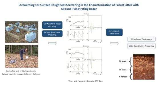
Accounting for Surface Roughness Scattering in the Characterization of Forest Litter with Ground-Penetrating Radar

by
Frédéric André
1,†,
François Jonard
1,2,*,†,
Mathieu Jonard
1,
Harry Vereecken
2 and
Sébastien Lambot
1
1
Earth and Life Institute, Université catholique de Louvain, 1348 Louvain-la-Neuve, Belgium
2
Agrosphere (IBG-3), Institute of Bio- and Geosciences, Forschungszentrum Jülich GmbH, 52425 Jülich, Germany
*
Author to whom correspondence should be addressed.
These authors contributed equally to this work.
Remote Sens. 2019, 11(7), 828; https://doi.org/10.3390/rs11070828
Submission received: 15 February 2019 / Revised: 31 March 2019 / Accepted: 3 April 2019 / Published: 7 April 2019
(This article belongs to the Special Issue Recent Progress in Ground Penetrating Radar Remote Sensing)

Abstract

:
Accurate characterization of forest litter is of high interest for land surface modeling and for interpreting remote sensing observations over forested areas. Due to the large spatial heterogeneity of forest litter, scattering from litter layers has to be considered when sensed using microwave techniques. Here, we apply a full-waveform radar model combined with a surface roughness model to ultrawideband ground-penetrating radar (GPR) data acquired above forest litter during controlled and in situ experiments. For both experiments, the proposed modeling approach successfully described the radar data, with improvements compared to a previous study in which roughness was not directly accounted for. Inversion of the GPR data also provided reliable estimates of the relative dielectric permittivity of the recently fallen litter (OL layer) and of the fragmented litter in partial decomposition (OF layer) with, respectively, averaged values of 1.35 and 3.8 for the controlled experiment and of 3.9 and 7.5 for the in situ experiment. These results show the promising potentialities of GPR for efficient and non-invasive characterization of forest organic layers.

Graphical Abstract

1. Introduction

Accurate soil surface characterization is essential for the understanding and the modeling of the various processes occurring at the soil-vegetation-atmosphere interface. In particular, soil water content is a fundamental soil state variable in many fields such as hydrology, soil and water resource management or meteorology. Therefore, L-band (1–2 GHz) remote sensing missions like the ESA Soil Moisture and Ocean Salinity (SMOS) or the NASA Soil Moisture Active Passive (SMAP) satellites have been especially designed for the large scale measurement of this key variable [1,2]. Yet, though soil water content estimations with reasonable accuracy are generally obtained from remote sensing data over grasslands and crops [3,4], much larger uncertainties are usually associated with corresponding estimates for forested areas mainly due to the presence of litter on the forest floor [5,6,7]. Indeed, this layer, consisting essentially of shed vegetative parts and organic matter in various stages of decomposition at the soil surface, was found to significantly reduce the sensitivity of the remote sensing signal to the water content of the underlying mineral soil [5,7,8,9,10]. Furthermore, forest litter is also acknowledged to have a significant influence on the backscattered signal of synthetic aperture radar (SAR) used in other microwave remote sensing missions (e.g., Sentinel-1) to determine biophysical properties of forest canopies, leading potentially to inaccuracies and bias in the estimations of canopy parameters (e.g., tree height, canopy architecture, aboveground biomass and water content) [11,12,13]. Consequently, the presence of litter has to be accounted for in the electromagnetic models used to process microwave remote sensing data acquired over forests [8,10,14,15,16]. Knowledge of the electromagnetic properties and their spatiotemporal dynamics of this compartment is required for proper modeling of remote sensing microwave data. However, although the effects of the forest litter on microwave remote sensing are now well recognized and despite the research efforts undertaken over the past few years in that direction (e.g., [14,17]), in situ experiments related to this topic remain scarce.
Besides, soil organic layers are important components of forest ecosystems, notably with regard to carbon balance or to water and nutrient cycling as well as to soil protection or population dynamics of ground vegetation and soil fauna [18,19,20,21,22,23,24]. These matters require detailed characterization of humic horizons, especially in the context of global warming and climate change feedback effects [25,26]. In addition, forest litter thickness and composition usually present a relatively large spatial variability under the combined influence of stand characteristics with climatic, biological and anthropogenic factors [27,28,29,30]. Nevertheless, methods traditionally used to characterize forest litter and to capture its spatial variability are tedious, time consuming and disturbing or destructive.
Given its ability to provide efficient and non-invasive characterization of soil and materials, ground penetrating radar (GPR) appears as being a particularly convenient tool to characterize litter layers with fine spatial and/or temporal resolutions over relatively large areas. Moreover, this geophysical technique could also be used to both study the effects of litter on the microwave signal from proximal measurements and determine litter constitutive properties. This information could then subsequently be used in remote sensing radiative transfer models. Nevertheless, few studies have investigated the potentialities of GPR to characterize litter. In a first study, Winkelbauer et al. [31] successfully retrieved the total thickness of humus horizons and could reconstruct its spatial variability using a time domain GPR system equipped with a 800 MHz centre-frequency antenna. However, these authors could not delineate the different humus horizons, presumably as a result of the rather low operating frequency combined with the limited dielectric contrast between horizons and their generally small thicknesses. More recently, using an off-ground ultrawideband stepped-frequency continuous-wave (SFCW) GPR and resorting to full-wave inversion of the radar data [32], André et al., demonstrated the ability of the technique to retrieve litter layer thicknesses and to provide reliable estimates of their constitutive properties in both controlled [33] and in situ [34] conditions.
In other respects, surface roughness may strongly affect backscattered electromagnetic signals by engendering diffuse reflection, also referred to as scattering, while most of the energy would be reflected in the specular direction on a smooth surface. As a result, either for remote or proximal sensing data, surface roughness effects have to be considered in signal processing and have been a matter of intense research work for many years. Rough surface scattering may be modeled through either semi-empirical, analytical or numerical approaches. Semi-empirical methods consist of simple physically-based equations with parameters fitted experimentally and their validity is usually restricted to the conditions from which they have been established. Analytical approaches are based on a physical description of wave scattering on a rough surface using approximations and/or assumptions so as to derive close form equations for modeling the backscatter, and their applicability is thereby limited to the conditions for which these assumptions are valid. In contrast, numerical methods solve directly the Maxwell equations for a numeric physical reconstruction of the investigated surface to provide the results of the scattering on that surface. Therefore, numerical methods are more accurate than the two former approaches and are usually considered as references. Yet, they are much more computationally intensive methods, which limits their usage compared to semi-empirical and analytical approaches, especially in an inversion framework. In the specific case of off-ground GPR, Jonard et al. [35] combined the full-waveform GPR model of Lambot et al. [32] with the Ament roughness model derived from the Kirchhoff scattering theory [36,37]. Despite the abundant literature on surface roughness effects on electromagnetic signals, only a few studies focused on the scattering and emission from litter layers. Among these works, Della Vecchia et al. [38] included the contribution of litter in forest radiative transfer models using an effective medium approach by considering the litter layer as a mixture of leaves, water and air and they accounted for its roughness through IEM, while Lawrence et al. [39] used a FEM approach for modeling rough surface scattering and emission of soil and litter layers. André et al. [33,34] considered frequency dependence of litter effective electrical conductivity to account for the effects of both relaxation and scattering phenomena on the radar signal.
In the present paper, we apply the combined full-waveform and roughness radar model proposed by Jonard et al. [35] to the GPR data from the controlled and in situ experiments of André et al. [33,34] in order to investigate the ability of the approach to properly reconstruct litter horizons, and to evaluate thereby the potentiality of the technique to provide quantitative characterization of litter for both surface roughness and horizon constitutive properties. The results of the present approach including a physical description of scattering through a roughness model are compared with those obtained previously by considering frequency dependence of effective electrical conductivity of litter to account for scattering together with dielectric losses.

2. Material and Methods

This section describes the experimental setups, the electromagnetic model used to process the GPR data and the statistics considered to analyze the results. The symbols used to represent the different parameters are listed in Table 1 along with a brief description of their meaning.

2.1. Experimental Setups

Both the controlled and the in situ experiments were carried out in the “Bois de Lauzelle”, located nearby the city of Louvain-la-Neuve in central Belgium.
The controlled experiment was performed on 25 July 2012 within a beech stand situated on a leached brown soil (Luvisol according to the Food and Agricultural Organization of the United Nations (FAO) classification) with a moder type humus composed of well-developed recently fallen (OL) and fragmented (OF) litter layers [40]. The setup consisted in a square wood frame 1.0 m × 1.0 m wide and 0.2 m high placed on a flat area after removal of the organic horizons, the mixed organo-mineral A horizon constituting therefore the bottom layer (lower half-space in the model). A first radar measurement was performed without the litter layers to characterize the properties of this A horizon. Litter was then collected in the surrounding area and was placed into the wood frame according to three different litter configurations: (1) a single OL layer, (2) a single OF layer and (3) an OF layer overlaid by an OL layer (Figure 1). For each configuration, litter was progressively added so as to consider different litter thickness levels, namely, nine OL levels (with 2.5, 3.8, 5.4, 6.3, 7.8, 8.9, 10.3, 12.8 and 17.0 cm for OL thickness), four OF levels (with 2.6, 3.9, 5.0 and 6.3 cm for OF thickness) and four OL-OF levels (with 4.7, 6.0, 7.2, and 8.8 cm for OL + OF thickness). A GPR measurement was performed after each litter addition so as to acquire radar data for each level and the height of the radar antenna above the litter surface ( h 0 ) and the litter thickness ( h 1 ) were then measured to the nearest millimeter with a measuring tape using a cardboard plane placed horizontally at the litter surface: h 0 corresponds to the vertical distance between the antenna aperture and the cardboard, while h 1 was determined by subtracting from the wood frame height (i.e., 0.2 m, see above) the vertical distance measured between the cardboard and the wood frame top. The litter volumetric and gravimetric water contents were determined using the oven-drying method at 105 ° C for at least 48 h. The measured volumetric water content amounted to 1.4% and 22.8% for the OL horizon and the OF horizon, respectively.
The in situ experiment was conducted on 19 June 2014 along a 100 m length transect crossing stands of various deciduous and coniferous tree species, namely, pure western hemlock (Tsuga heterophylla (Raf.) Sarg.) stands, a mixed hemlock and common beech (Fagus sylvatica L.) stand, a clearing, a mixed deciduous stand with common beech, northern red oak (Quercus rubra L.) and pedunculate oak (Quercus robur L.), and a Norway spruce (Picea abies (L.) H. Karst) stand. GPR measurements and litter ground truth data were collected at 21 locations along the transect, in situations contrasting in terms of litter thickness and species composition. The encountered humus types ranged from acidic mull under the deciduous trees to moder in the coniferous stands.
GPR measurements were carried out at three different positions around each location so as to capture the local spatial variability of litter properties. In addition, radar measurements were repeated twice at each position in order to integrate measurement errors likely to arise from small movements of the antenna held manually during data acquisition (see Section 2.2). After radar measurements, litter was collected by monolith sampling at each GPR measurement location using a square 0.09 m 2 area metal frame and placed in hermetic plastic bags for bulk density and volumetric water content determination in the laboratory. OL and OF litter layer thicknesses were measured to the nearest millimeter in the middle of each side of the sampling square, using a measuring tape. Finally, litter was removed over wider areas (c.a., 1.0 m × 1.0 m) centered on each sampling location and a second set of radar data was collected for characterizing the properties of the organo-mineral A horizon, which was considered as the bottom layer of the litter profile (i.e., lower half-space of the electromagnetic model configuration). Contrary to the controlled experiment, both the OL and OF litter layers were systematically present for these natural, undisturbed, situations and only the OL-OF litter configuration (see Figure 1c) was considered when processing the GPR data in the presence of litter.
Pictures of the setups for both experiments are presented in Figure 2. We refer to [33] and to [34] for detailed descriptions of the controlled and in situ experiments, respectively.

2.2. Radar Measurements

For both the controlled and the in situ experiments, the radar measurements were carried out using an ultra wideband stepped-frequency continuous-wave radar connected to a transmitting and receiving doubled-ridge horn antenna (BBHA 120 A, Schwarzbeck Mess-Elektronik, Schönau, Germany) operating at about 30 cm above the medium. The antenna has a 14 × 24 cm 2 aperture area and is 22 cm high. Its nominal frequency range is 0.8 to 5.2 GHz and the isotropic gain ranges from 4.4 to 14.0 dBi. The antenna was connected to the reflection port of a vector network analyzer (VNA, ZVL, Rohde & Schwarz, Munich, Germany) with a high quality N-type 50- Ω coaxial cable. The VNA was calibrated at the connection between the coaxial cable and the antenna using a standard Open-Short-Match (OSM) calibration kit. The frequency-dependent complex ratio S 11 ( f ) between the returned and the emitted signals was measured sequentially at 734 evenly stepped frequencies from 0.8 to 5.2 GHz with a frequency step of 6 MHz, f being the frequency. For the the controlled experiment, the antenna was fixed on a rigid fiberglass tube to ensure its stability during the measurements. In contrast, the antenna was held manually by the operator during the in situ experiment, the forest floor micro-relief and the rather high stand density making difficult the use of an antenna support in this case.

2.3. Radar Data Processing

2.3.1. Radar Model

The antenna being located in the far-field region in both experiments (see [41]), the distribution of the backscattered field over the antenna aperture is homogeneous and the far-field model proposed by Lambot et al. [32] can be applied. In this approach, the antenna is described using (1) a single point source and receiver located at its phase centre and (2) global reflection and transmission, frequency-dependent coefficients to account for the internal antenna variations of impedance. The radar equation is formulated in the frequency domain as [32,42]:
S 11 ( f ) = b ( f ) a ( f ) = R 0 ( f ) + T s ( f ) G x x ( f ) T i ( f ) 1 G x x ( f ) R s ( f )
where S 11 ( f ) is the measured complex ratio between the backscattered b ( f ) and the incident a ( f ) fields at the VNA reference plane, R 0 ( f ) is the global reflection coefficient of the antenna in free space, T i ( f ) and T s ( f ) are the global transmission coefficients for the field incident from the VNA reference calibration plane onto the point source and for the field incident from the layered medium onto the field point, respectively, accounting for the gain and phase delay, and R s ( f ) is the global reflection coefficient for the field incident from the layered medium onto the field point leading in particular to the interactions between the antenna and the medium. G x x ( f ) is a Green’s function representing the response of the air-subsurface system and is formulated as an exact solution of the 3-D Maxwell’s equations for electromagnetic waves propagating in planar layered media. It is defined as the x-directed component of the reflected electric field for a unit-strength x-directed electric source and it is derived using a recursive scheme to compute the transverse electric (TE) and magnetic (TM) global reflection coefficients of the multilayered medium in the spectral domain [43,44]. The transformation back to the spatial domain is performed by evaluating numerically a semi-infinite integral using a fast evaluation method [45]. The antenna transfer functions are determined from radar measurements over well characterized medium configurations for which the corresponding Green’s functions can be computed [32,46].
Rearranging Equation (1), it is possible to filter the antenna effects out of the raw radar data and obtain in this way the observed Green’s function G x x m e a s ( f ) corresponding to the medium response only:
G x x m e a s ( f ) = S 11 ( f ) R 0 ( f ) S 11 ( f ) R s ( f ) + T ( f ) R 0 ( f ) R s ( f ) ,
where T ( f ) = T s ( f ) T i ( f ) .

2.3.2. Model Configurations

The GPR data acquired directly above the A horizon (i.e., before placing litter in the wood frame for the controlled experiment, and after litter removal in the in situ experiment) were processed considering a two-layer electromagnetic model in order to characterize the A horizon. The first layer represents the air layer between the antenna and the soil surface. Its electrical conductivity and relative dielectric permittivity values were set to the theoretical values σ 0 = 0 Sm 1 and ε r , 0 = 1, respectively, and its thickness corresponds to the sum of the distance between the antenna phase center and its aperture ( p c = 7.14 cm) with the antenna height ( h 0 ). The second layer is the lower half-space and represents the A horizon. Its electrical conductivity was set to σ A = 0 Sm 1 , referring to the findings of [47]. Accordingly, the corresponding radar data were inverted for h 0 and A horizon relative dielectric permittivity ( ε r , A ) focusing on the surface reflection (see Section 2.3.3).
The model configuration used to analyze the GPR data acquired in the presence of litter was adapted as a function of the litter configuration. A three-layer electromagnetic model was considered for the single OL layer and the single OF layer configurations of the controlled experiment, while a four-layer model was adopted to process the data for the controlled OL-OF configuration as well as those of the in situ experiment. As for the A horizon configuration, the first layer corresponds to the air layer between the antenna phase center and the litter surface and the lower half-space represents the A horizon. The relative dielectric permittivity of this latter horizon was set to the value retrieved from inversion of the signal in the absence of litter. The intermediate layer(s) correspond(s) to OL and/or OF litter.
André et al. [33,34] showed that proper modeling of radar data collected above litter requires frequency dependence of medium properties to be considered in order to account for both scattering and dielectric losses occurring within litter horizons. In these works, radar data were successfully reproduced by the electromagnetic model when the frequency dependence of litter effective electrical conductivity was described by the following linear equation:
σ ( f ) = σ 0.8 GHz + a ( f 0.8 × 10 9 ) ,
where σ 0.8 GHz is the reference electrical conductivity at 0.8 GHz and a is the linear variation rate of σ ( f ) . Furthermore, as evidenced by the findings of the previous studies, σ 0.8 GHz was considered as equal to 0 Sm 1 . Indeed, dielectric losses due to relaxation of water molecules become essentially significant above 1 GHz, the relaxation frequency of free water being around 17 GHz.
Jonard et al. [35] adapted the electromagnetic model to account for surface roughness. In this model, the scattering losses in the specular direction due to the reflection on the rough surface are considered by multiplying the global reflection coefficients by a scattering loss factor ( ρ ), which is based on the Rayleigh parameter expressed as a function of frequency and is formulated as:
ρ = e 1 2 4 π s r cos γ i λ 2 ,
where s r is the standard deviation of the surface height, γ i is the incidence angle and λ is the free space wavelength of the incident wave. Then, the modified TE- and TM-mode reflection coefficients, R T E R and R T M R , accounting for the reduction of the energy reflected in the specular direction are defined as:
R T E ( T M ) R = ρ R T E ( T M ) F ,
with R T E F and R T M F being the corresponding global reflection coefficients for a smooth surface. Equation (5) assumes a Gaussian distribution for the surface heights with negligible sharp edge and shadowing effects. The model also considers the absence of multiple scattering [37].
For the present study, the incidence is normal ( γ i = 0 ) and the model is applied to the spectral-domain global reflection coefficients of the first interface (i.e., litter surface) of the layered medium. Both the controlled and the in situ data sets were processed using this approach in order to investigate the ability of the model to describe radar data collected above litter and to evaluate its performances with regard to the preceding approach. Several model parameterizations were tested, considering either exclusively the roughness model to account for the dispersive properties of litter or applying it jointly with the linear frequency dependent model presented in Equation (3). In all cases, the magnetic permeability μ of each layer was assumed as equal to that of free space (i.e., μ 0 = 4 π × 10 7 Hm 1 ), which holds for nonmagnetic materials as found in litter and soils in most environments [48,49].

2.3.3. Model Inversion

As aforementioned, radar data inversion for the dielectric permittivity of the A horizon after litter removal was carried out in the time domain by focusing on the surface reflection, adopting the approach proposed by [47]. According to this procedure, the objective function to be minimized is formulated as:
ϕ 1 ( b ) = | g x x m e a s g x x m o d | T | g x x m e a s g x x m o d | ,
where g x x m e a s ( t ) = g x x m e a s ( t ) | t m i n t m a x and g x x m o d ( t , b ) = g x x m o d ( t , b ) | t m i n t m a x are, respectively, the observed and simulated Green’s functions in the time domain over the [ t m i n t m a x ] time window including the surface reflection, b is the vector of parameters to be estimated (i.e., h 0 and ε r , A ). Optimization was carried out using the local Levenberg–Marquardt algorithm [50].
Inversion of the GPR data collected above litter was performed in the frequency domain by minimizing the objective function defined as follows:
ϕ 2 ( b ) = | G x x m e a s G x x m o d | T | G x x m e a s G x x m o d | ,
where G x x m e a s ( f ) and G x x m o d ( f , b ) are, respectively, the observed and simulated Green’s functions in the frequency domain. In this case, the optimized parameters b correspond to the electromagnetic properties and the thicknesses of the litter layers (i.e., ε r , OL , ε r , OF , a OL , a OF , h OL , h OF , s r ) and the antenna height h 0 . Besides, a simplified model was also tested by neglecting a OL and/or a OF , in order to investigate the relevance of accounting for the frequency dependence of the effective electrical conductivity of the litter layer(s) when applying the roughness model as well as to reduce the number of unknowns. Given the complex topography of the objective function and the large dimension of the parameter space, inversion of these data was carried out by combining sequentially the global multilevel coordinate search (GMCS) algorithm [51] with the Levenberg–Marquardt algorithm [52,53].

2.4. Statistics

For result comparison, the same statistical tests and measures of agreement as reported by André et al. [34] were used to examine the correspondence between estimated and measured values of litter layer thicknesses for the in situ experiment. Statistical tests consisted in a paired Student’s t-test and in a linear regression between two sets of values and the selected measures of agreement were the Pearson’s correlation coefficient (r), the root mean square error ( R M S E ) and the fractional bias ( F B ) defined as follows by Janssen et al. [54]:
F B = E ¯ M ¯ 1 / 2 ( E ¯ + M ¯ ) ,
where E ¯ and M ¯ are, respectively, the means of the estimated and measured values of the considered parameter.
The paired Student’s t-test and F B quantify the bias between compared values. The regression analysis tests for the significance of the deviation of the intercept and of the slope from 0 and 1, respectively. If the slope is close to 1, an intercept significantly different from zero reflects the presence of systematic differences between compared values, while deviation of the slope from 1 indicates proportional bias. Linear regression coefficients were determined through total least squares to account for the fact that both the dependent and the independent regression variables (i.e., the estimated and measured litter thicknesses) were associated with errors [55]. Confidence intervals of regression coefficients were established using the bootstrap percentile method considering 10,000 replicated computations [56]. According to this procedure, the lower and upper interval limits are, respectively, the 250th (10,000 × α /2) and the 9750th (10,000 × (1− α /2)) ordered values of the replications, α being the significance level (fixed to 0.05). Finally, the correlation coefficient quantifies the strength of the linear relationship between the two compared variables and the R M S E expresses the discrepancy between paired values.
Such statistics were not considered for the controlled experiment for which graphical comparisons of estimates with measurements and with previous results are more straightforward than for the in situ experiment given the lower number of observations and the better agreement found between measured and estimated litter thicknesses (see below).

3. Results and Discussion

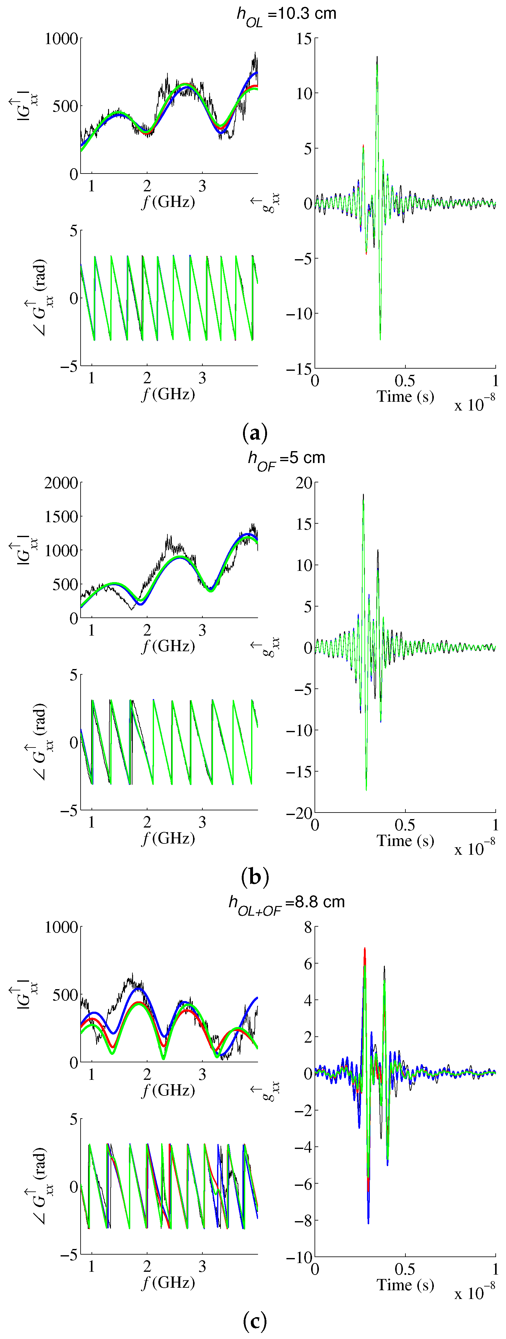
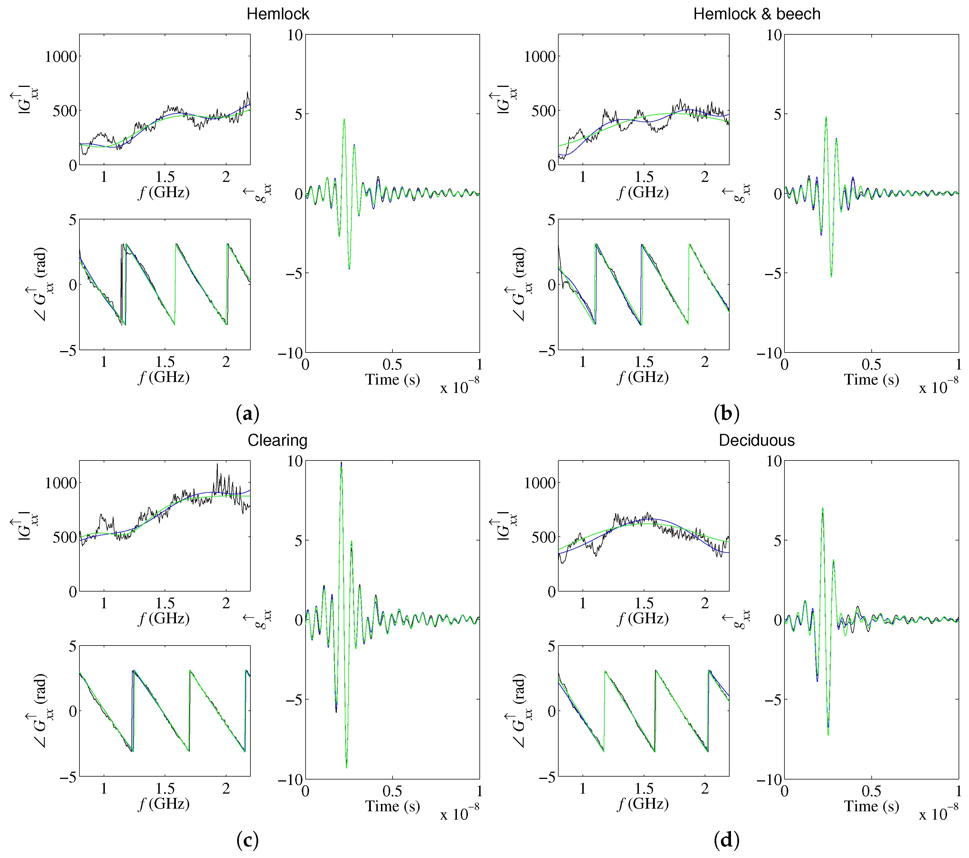
3.1. Radar Signal Modeling

Full-wave inversion of the GPR signal was used to evaluate the applicability of the proposed radar model accounting for surface roughness to forest litter characterization. Measured Green’s functions (see Equation (2)) and modeled Green’s functions obtained from radar data inversion are presented in Figure 3 and Figure 4 for the controlled and the in situ experiments, respectively. Modeled Green’s functions reported by André et al. [33,34] for the model considering only frequency dependence of litter effective electrical conductivity are also shown for comparison. Though the GPR data were acquired between 0.8 and 5.2 GHz, radar signal inversions focused over the 0.8–4 GHz and the 0.8–2.2 GHz bands for the controlled and the in situ experiments, respectively, due to the presence of noise in the data at higher frequencies. This noise would notably result from small movements of the antenna during the measurements, especially for the in situ experiment for which the antenna was held manually by the operator (see above).
For the controlled experiment, close correspondence is generally observed between the measured and the modeled Green’s functions, as illustrated in Figure 3 with data selected for each of the three considered litter configurations. In each case, the phase in the frequency domain and, as a result, the propagation time in the time domain are well reproduced by the model. On the other hand, some differences appear between the amplitudes of the measured and modeled Green’s functions, especially in the more complex cases (i.e., OL-OF configuration). These differences are particularly noticeable in the frequency domain, while in the time domain, quite good agreement is found for the main reflections and most of the discrepancies between measured and modeled Green’s functions are observed at larger propagation times, corresponding to the lower half-space. Besides, comparing modeled Green’s functions, good correspondence is also generally found between the model considering only frequency dependence of litter effective electrical conductivity (blue curves), the model accounting for both surface roughness and frequency dependence of litter effective electrical conductivity (red curves) and the model considering surface roughness only (green curves). Yet, pronounced discrepancies between model versions are sometimes observed, as notably in Figure 3c for the OL-OF configuration. These discrepancies mainly occur between the model considering only frequency dependence and the models accounting for surface roughness, while close correspondence is found between the two model versions including surface roughness (i.e., with or without consideration of frequency dependence). Comparison of the models through examination of the values of the objective functions at optimum parameter estimates ( ϕ 2 ) confirms the preceding observations and reveals that the models accounting for surface roughness often present smaller ϕ 2 values and, therefore, closer agreement than the model considering only frequency dependence of effective electrical conductivity (Figure 5a). Such observations would indicate the significance of accounting for surface roughness when modeling radar data acquired above forest litter. In contrast, the relatively small differences among both model versions including surface roughness suggest irrelevance of considering frequency dependence of litter effective electrical conductivity when accounting for roughness. This will be corroborated by analysis of the parameter inversion results (see Section 3.2). These findings are of interest for the characterization of litter layers from radar data as neglecting frequency dependence parameters a OL and a OF allows to reduce the complexity of the inverse problem, leading thereby to potentially more stable estimates of the other litter properties.
Based on the results from the controlled experiment showing irrelevance of considering frequency dependence of litter effective electrical conductivity when surface roughness is included in the electromagnetic model and for the sake of conciseness, only the model accounting exclusively for surface roughness was considered when processing GPR data from the in situ experiment. As for the controlled conditions, generally close correspondence between measured and modeled Green’s functions was found for in situ data, especially in the time domain and for the phase in the frequency domain while more noticeable discrepancies appear for the amplitude in the frequency domain. This is illustrated in Figure 4 with data from four contrasted situations along the measurement transect (i.e., pure hemlock stand, mixed hemlock-beech stand, clearing, and mixed deciduous stand). Similarly, good agreement is generally observed between the model accounting for frequency dependence of litter effective electrical conductivity proposed by André et al. [34] (blue curves) and the model considering surface roughness (green curves) though discrepancies between both models are also present, especially for the amplitude in the frequency domain. Contrary to the controlled experiment, the comparison of the two model versions based on the objective function values at parameter optimum shows no systematic ranking among the different measurement locations along the transect (Figure 5b). Moreover, as shown by the generally overlapping errors bars depicting the 95% confidence intervals for ϕ 2 , no significant differences are observed among performances of both model versions in terms of agreement with the data.

3.2. Estimates of Litter Properties

3.2.1. Litter Layer Thicknesses

Inversion estimates of litter layer thicknesses are compared to corresponding measured values in Figure 6 and Figure 7 for the controlled and the in situ experiment, respectively. For the controlled experiment, the results are distinguished for the different litter configurations using separate marker types, namely, triangles for single OL layer (see Figure 1a), squares for single OF layer (see Figure 1b) and circles for OL-OF litter (see Figure 1c). Furthermore, results are presented for the model proposed by André et al. [33] considering only frequency dependence of litter effective electrical conductivity (blue markers), for the model accounting for both surface roughness and frequency dependence of litter effective electrical conductivity (red markers) and for the model considering surface roughness only (green markers). For the in situ experiment, marker colors are used to distinguish the different stand compositions at measurement locations. As stated before, only the OL-OF litter configuration (see Figure 1c) was considered for this latter experiment.
For the controlled experiment, close correspondence is generally observed between measured litter thicknesses h 1 and corresponding inverse estimates (Figure 6a). R M S E values found when accounting for roughness only amount to 22.6 × 10 3 m, to 4.9 × 10 3 and to 8.0 × 10 3 for the OL, OF and OL-OF configurations, respectively.
The larger R M S E value for OL litter mainly results from systematic underestimation of litter thicknesses for this configuration. Differences in considering the position of litter surface between the model and for litter thickness ground truth measurements might explain these observations. Indeed, a cardboard plane placed on litter was used as a reference for litter surface for determination of litter thickness ground truth values (see Section 2.1). As a result, litter surface was assumed in this case as corresponding to the top of peaks of surface roughness. In contrast, in the models accounting for roughness, litter surface was considered as the average level of the roughness peaks and troughs, the roughness coefficient s r being defined as the standard deviation of the surface height. Therefore, thickness estimates provided by the model considering roughness are expected to have lower values than corresponding ground truth measurements. It is worth to note that the two models accounting for roughness, with and without consideration of frequency dependence of litter effective electrical conductivity, generally provide identical (i.e., to the neatest millimeter) thickness estimates. One exception is the case with the largest litter thickness for which the model considering roughness only provides a much lower thickness estimated value than the model accounting for both roughness and frequency dependence. This outlier point would presumably arise from an inversion problem. Similarly as for the comparison with the ground truth thickness values, the models accounting for roughness provide systematically lower estimates of OL litter thickness compared to the values retrieved by André et al. [33] with the model considering only frequency dependence of litter apparent electrical conductivity. In the latter model, litter surface is defined as the air-litter interface and the litter roughness peaks are then part of the litter layer thickness, which corresponds to the reference adopted to determine ground truth thicknesses. As a result, closer agreement ( R M S E = 8.5 × 10 3 m) was found by André et al. [33] between estimated and measured OL litter thickness than observed in the present study with the roughness model. Yet, adding estimations of roughness peak heights derived from s r coefficient to OL thickness estimates obtained when considering roughness improves the agreement with measured thickness values. This is illustrated in Figure 6a by the error bars representing 1.96 × s r which, according to the assumption of Gaussian distribution considered for surface height variations due to roughness, would correspond to the intervals containing 95% of the peak and trough amplitude values around the average surface height level. The upper limit of this interval is in most cases (except the outlier point) close to the 1:1 line and/or to the André et al. [33] thickness estimate values, indicating that “roughness thickness” would at least partly explain the underestimation of OL litter layer thickness noticed when accounting for roughness.
Contrary to the OL configuration, systematic h 1 underestimation is not found for the OF and OL-OF litter configurations for which good agreement between estimated and measured litter thickness values is observed. The absence of underestimation for the OF configuration would result from the lower levels of OF litter roughness as revealed by the smaller corresponding s r estimates compared with OL litter (see below). The explanation for the absence of underestimation is less obvious for the OL-OF configuration. It could notably arise from the larger complexity of the inverse problem compared with the single litter layer configurations due to the larger set of parameters to be estimated, potentially giving rise to larger uncertainties affecting the estimations. In other respects, compared to the model proposed by André et al. [33], OF and OL-OF litter thickness estimates from the models considering roughness show closer agreement with ground truth measurements, especially for the largest thickness levels. As already pointed out above when comparing the objective functions (see Section 3.1), such observations would indicate that accounting for roughness would allow for improved modeling of radar data collected over forest litter compared with the model based on frequency dependence of litter effective electrical conductivity, presumably as a result of a more physical description of the scattering phenomena occurring at the rough surface.
Regarding the individual OL and OF layers for the OL-OF litter configuration, poorer agreements are found between estimated and measured thicknesses h O L and h O F (Figure 6b,c). For the OL layer, such results could partly arise from the quite narrow range of thickness values considered for this configuration, which imperil the identification of any significant relationship between both sets of values. Besides, the relatively limited dielectric contrast between the OL and the OF litters (see below) leading to inaccurate delineation of the two layers through signal inversion may also explain the weak correspondence between thickness estimations and measurements, which is corroborated by the rather close correspondence found for total litter thickness h 1 for the same configuration (Figure 6a). Indeed, such a close correspondence for h 1 , defined as h O L + h O F , indicates that total litter layer is well reconstructed and, therefore, that overestimations observed for h O L are compensated by underestimations for h O F , and inversely.
Finally, it is worth noting that divergences between litter thickness estimations and corresponding ground truth values may also partly result from inaccuracies in the measurement of litter thicknesses. These inaccuracies have been quantified below for the in situ experiment through repetitions of the litter layer thickness measurements at each location.
For the in situ experiment, plots presenting estimated litter layer thickness as a function of ground truth values present larger dispersion of the points around the 1:1 line than observed for the controlled experiment (Figure 7). The corresponding statistics are presented in Table 2 for both the complete data set and a restricted data set for which the two points presenting extreme high measured values for h OL and h 1 in the mixed hemlock-beech stand were not considered to avoid misinterpretation of the results due to the predominant influence of these two points on the statistics compared with the other observations.
R M S E values found for h OL are close to 1 cm while values ranging from 1.5 cm to 2 cm are observed for h OF and h 1 . For h OL , these R M S E values are in agreement with that found above for the controlled experiment as well as with those reported by André et al. [33,34]. Regarding h OF and h 1 , R M S E values correspond with results for the in situ experiment using the model considering only frequency dependence of litter effective electrical conductivity [34], while they are up to three times higher than the values obtained for the controlled experiment (see above and [33]). On the other hand, in contrast to R M S E , correlation coefficients r indicate closer agreement between estimated and measured thicknesses for h 1 and h OF than for h OL . Looking at the restricted data set so as to avoid the strong influence of the two extreme points, r values found for h OL , h OF and h 1 are 0.352, 0.628 and 0.709, respectively. As already mentioned above for the OL-OF litter configuration of the controlled experiment, the nonsignificant correlation values observed for h OL would notably result from the quite narrow range of values encountered for this parameter. Indeed, the range of values for h OL is of the same order of magnitude as its measurement and estimation errors as depicted in Figure 7a by the horizontal and the vertical error bars representing 95% confidence intervals to average measured and estimated values, respectively. It also explains the nonsignificant values obtained for the corresponding regression coefficients. For h OF , points are distributed around the 1:1 line for the lowest thickness levels corresponding to the deciduous stand situations, indicating on average good agreement between measurements and estimations in these cases. In contrast, as h O F increases, a tendency to underestimate the parameter is observed (Figure 7b). As a result, an intercept close to 0 and a slope lower than 1 are found for the regression between estimated and measured h OF . A pattern similar to that of h OF is observed for total litter thickness ( h 1 ) but with a regression slope closer to 1 (Figure 7c), revealing that underestimations noticed above for h OF are partly compensated by overestimations for h OL and suggesting thereby inaccurate delineation of OL and OF litter horizons through GPR signal inversion. Yet, as confirmed by the F B and paired t-test statistics showing negative values, though non significant, a general tendency to underestimate litter thickness occur when surface roughness is accounted for in the electromagnetic model, while it was not the case when only frequency dependence of litter effective electrical conductivity was considered [34]. These observations evoke the results presented above for h OL in controlled conditions, showing that underestimation of litter layer thickness could be corrected through consideration of the surface roughness coefficient estimates ( s r ). Applying the same correction to in situ h 1 estimates substantially improves the agreement between estimated and measured values, both visually (Figure 7d) and statistically with regression slopes getting closer to 1 and a noticeable decrease of t-ratio and F B values compared with uncorrected h 1 . The correlation coefficients also slightly increase (Table 2). Nevertheless, in spite of the relatively good agreement between corrected estimations and measurements of h 1 , significant discrepancies between both sets of values are found in some cases, which may arise from a limited dielectric contrast between litter and the A horizon at these locations as often observed along the measurement transect (Figure 9a). A particularly marked h 1 underestimation is observed for a point of the mixed hemlock-beech stand presenting the largest values for litter thickness. Besides a weak dielectric contrast among horizons, the presence of large roots in the OF horizon may also explain such an observation. Indeed, these large roots may significantly affect the GPR signal while the electromagnetic model used in the present study consider litter as a planar layered medium and does not allow to account for such local objects, which could therefore influence the reconstruction of litter horizons through GPR data inversion. Finally, as already aforementioned for the controlled experiment, it is important to note that, aside these modeling errors, local spatial variations of litter layer thicknesses combined with difficulties in their visual delineation may also lead to measurement errors giving rise to divergences between thickness estimates and ground truth values. Significant measurement errors occurred in some cases as attested by the rather large horizontal error bars sometimes observed in Figure 7, representing confidence intervals to the average measured thickness values.
These results are similar to those obtained when considering only frequency dependence of litter effective electrical conductivity [34], the most noticeable changes being the higher values generally found in the present study for the correlation coefficients between estimated and measured thicknesses. Therefore, taking into account the effect of surface roughness, the electromagnetic model did not substantially improve the retrieval of litter layer thicknesses. Yet, accounting for this effect should potentially allow for a more physical description of scattering due to litter roughness, leading thereby to improved modeling of the GPR signal, as already pointed out above when comparing the objective functions (see Section 3.1). This will be further investigated in the next section by examining estimates of litter constitutive properties.

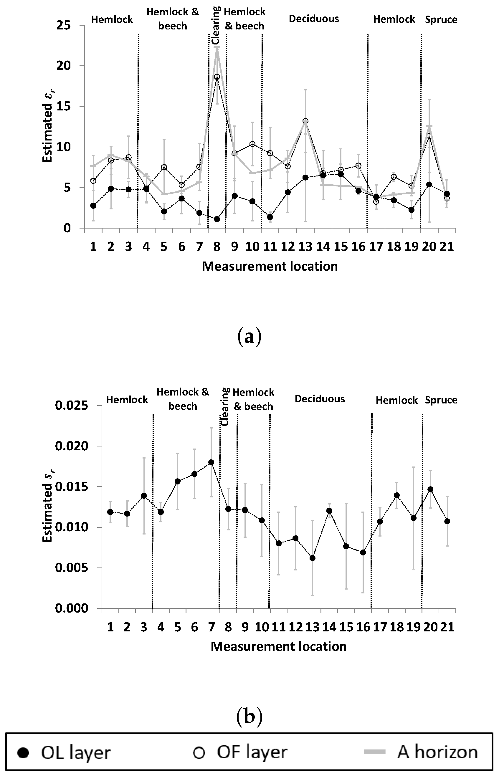
3.2.2. Litter Constitutive Properties

Estimates of litter electromagnetic properties retrieved from GPR data inversion are presented in Figure 8 and Figure 9 for the controlled and the in situ experiments, respectively.
For the controlled experiment, parameter estimates are plotted as a function of measured litter thickness. As above, the results are distinguished for the different litter configurations using separate marker types and estimates from the models accounting for surface roughness with (red markers) or without (green markers) consideration of frequency dependence of litter effective electrical conductivity are compared with results reported by André et al. [33] considering frequency dependence only (blue markers).
Estimates of OL litter relative dielectric permittivity ( ε r , OL ) when accounting for roughness show quite stable values for all litter thickness levels of the OL configuration, except for the largest thickness case for which a much higher estimated value is observed when considering roughness only (Figure 8a). Excluding this outlier point, ε r , OL estimates average out to 1.35, which is in accordance with the average value of 1.19 obtained by André et al. [33] without accounting for roughness. In contrast, ε r , OL estimates for the OL-OF configuration are often larger than corresponding values found by André et al. [33]. Inaccurate delineation of OL and OF horizons leading to overestimation of the thickness of the OL layer thickness, which thereby encroaches on the OF layer presenting higher relative dielectric permittivity values (see below), may explain these results. The fact that these observations occur only when accounting for roughness might arise from limited OL layer thicknesses (around 2 cm) considered for the OL-OF configuration. Indeed, values sometimes up to more than 1 cm retrieved for the estimates of the surface roughness coefficient s r would indicate that, in these cases, most of the layer thickness is considered as part of roughness itself by the model. This may induce a tendency to overestimate OL layer thickness when reconstructing horizons through GPR signal inversion. Yet, this explanation essentially holds for the observation OL-OF with the penultimate largest OL-OF thickness level, as overestimation of h OL accompanied by marked underestimation of h OF are found in that case only (see Figure 6b,c). Another possible explanation would be less stable parameter estimates associated with the higher complexity of the inverse problem given the rather large number of parameters to be estimated. Regarding OF litter, ε r , OF estimates for the OF and the OL-OF configurations are generally within similar ranges of values though a bit lower for OL-OF, with averages of 5.4 (4.27 without considering the estimation for the last observation of the OF configuration which appears to be an outlier) and 3.46, respectively (Figure 8b). These results are in agreement with findings of André et al. [33]. As already discussed by these authors, the higher values observed for ε r , OF compared to ε r , OL should at least partly result from both the higher water content and the higher density of OF layer.
Whatever the litter configuration, values retrieved for the rate of variation of effective electrical conductivity with frequency (a) are generally much lower for the model accounting for both surface roughness and frequency dependence compared with the model of André et al. [33] considering frequency dependence only with, in most of the cases, a estimates for the former model close to the lower bound of the optimization interval for this parameter (i.e., a = [10 13 10 8 ] SHz 1 m 1 ) (Figure 8c). Furthermore, the few cases for which a estimates from the model considering roughness are in agreement with values reported by André et al. [33] generally present estimations of surface roughness coefficient ( s r ) equal or close to 0 m (Figure 8d). Such observations would indicate that the electromagnetic phenomena considered through parameter a in the André et al. model, or at least the major part of them, are accounted for by coefficient s r when roughness is included in the model. This would mean that dielectric losses presumed as occurring in OF litter by André et al. [33,34], notably due to its higher water content compared to OL litter, would also be accounted for by coefficient s r , in addition to scattering resulting from surface roughness. Therefore, these results suggest that scattering and dielectric losses could generally not be characterized apart even when considering roughness and frequency dependence together in the model, both phenomena being accounted for either through parameter a or, as in most cases here, through coefficient s r .
Estimations of surface roughness coefficient s r for the OL configuration range from 0.4 cm for the lowest thickness level up to more than 1.0 cm for the largest ones, though quite stable values around 0.7 cm are observed for the intermediate thicknesses (Figure 8d). In contrast, for the OF and OL-OF configurations, a continuous increase of s r estimates is observed as litter thickness increases. For the OF configuration, s r estimates remain quite small with values increasing from 0 cm for the smallest litter thickness to 0.6 cm for the largest one. Such small values for the roughness coefficient may be attributed to the relatively smoother surface of OF litter compared with OL litter. Estimates of s r for the OL-OF configuration vary from 0 cm to 1.1 cm, which is in agreement with the range of values observed for the same coefficient for the OL configuration. In other respects, these increasing values of the roughness coefficients with OF and OL-OF litter thickness correspond to similar trends reported by André et al. [33] for parameters a for the same litter configurations (see Figure 8c). As already suggested above when discussing results for a estimates, this might further indicate that coefficient s r explains at least a part of the signal information initially accounted for by parameter a in the model version proposed by André et al. [33].
For the in situ experiment, parameter estimates are presented in Figure 9 as a function of measurement location along the transect.
Variations of the estimates of litter relative dielectric permittivity ( ε r ) along the transect show rather similar general patterns for both the OL and the OF layers, though variations are much pronounced for the OF layer (Figure 9a). Furthermore, values retrieved for the OL layer ( ε r , OL ) are in most cases lower than estimations for the OF layer ( ε r , OL ) at the corresponding location, with average values of 3.9 and 7.5, respectively. As already pointed out and discussed in the previous works [33,34], such differences of dielectric permittivity both among litter layers and among measurement locations should be at least partly ascribed to, respectively, vertical and horizontal spatial variations of physical litter properties, such as water content and bulk density. Yet, these differences are generally not significant due to the quite large variability of ε r estimates observed for most locations as shown by the 95% intervals to the estimates represented by the errors bars. This local variability of the estimates would itself also partly result from contrasted litter properties among the positions used as pseudoreplicates around each measurement location (see Section 2.1).
As presented in Figure 9b, estimates for the surface roughness coefficient s r show strong variations along the transect, in particular with generally lower values, around 0.7 cm, observed for the deciduous stand compared with the other measurement locations which are all characterized by the presence of coniferous species, except the clearing. These differences between deciduous and coniferous species might notably arise from contrasted litter thicknesses, the former species presenting the thinnest litter layers (see Figure 7). Such a positive effect of litter thickness on s r is consistent with the increasing estimated values of this parameter as litter thickness increases observed above for the controlled experiment (see Figure 8d). Finally, s r estimates around 0.7 cm for the deciduous stand are in agreement with corresponding estimates for the controlled experiment, concerning also a deciduous species, namely, beech.

4. Conclusions and Perspectives

A full-waveform radar modeling approach combined with the Ament roughness model was applied to radar data collected above litter in order to investigate its ability to provide quantitative characterization of forest floor organic layers in terms of their surface roughness and their constitutive properties. Radar data were acquired using an ultrawideband (0.8–4.0 GHz) off-ground GPR system both over artificially reconstructed litter horizons and over in situ, undisturbed, litter in stands of various tree species. The radar model used to invert the data considers all antenna effects, including antenna-medium interactions, and describes wave propagation in a three-dimensional layered medium using Green’s functions. The performances of the proposed combined full-waveform and roughness radar model are compared with those of a similar approach adopted in previous works by considering frequency dependence of litter effective electrical conductivity to account for litter scattering properties instead of a roughness model.
For both the controlled and the in situ experiments, the proposed modeling approach successfully reproduced radar data, showing agreement between measured and modeled signals at least equivalent and even often better than that obtained previously using the effective electrical conductivity frequency dependent model. Such improved performances for the present approach would arise from a better physical description of scattering through the roughness model than when considering frequency dependence of litter effective electrical conductivity. Litter thickness was generally retrieved with accuracies around 1 cm for the OL layer and around 1.5 cm for the OF layer as well as for the total litter in cases where both horizons were present, which corresponds to the accuracy levels reported in the previous studies. Yet, in the present study, such precisions were reached provided correction of the estimations for litter thickness by the corresponding values retrieved for the surface roughness coefficient. Estimates for this coefficient averaged to 0.7 cm and 1.3 cm for deciduous and coniferous litters, respectively. In other respects, when litter consisted of two overlaid OL and OF horizons, inaccurate delineation of both layers was generally observed at least partly due to limited dielectric contrast between OL and OF litter, as also mentioned in previous works. Besides, inversion of radar data also provided reliable estimates of litter electromagnetic properties with relative dielectric permittivities of OL and OF litter averaging, respectively, 1.35 and 3.8 for the controlled experiment and 3.9 and 7.5 for the in situ, which are in agreement with corresponding findings using the litter effective electrical conductivity frequency dependent approach.
These results show the promising potentialities of GPR for efficient and non-invasive characterization of forest organic layers. It could notably be used in ecological studies as an alternative to the time consuming and disturbing conventional methods used for humus description and sampling in other to capture the spatial and/or temporal variability of litter characteristics over extended areas. Furthermore, litter electromagnetic and scattering properties as provided by GPR signal inversion constitute valuable information for the processing of remote sensing data collected over forested areas, to be used either as direct inputs of the remote sensing models or as reference data for the calibration and the validation of their litter module.

Author Contributions

F.A., F.J. and M.J. ellaborated the methodological approach. F.A. and F.J. analyzed the data. F.A., F.J., M.J. and S.L. provided scientific expertise. H.V. acquired funding for the project. F.A. and F.J. wrote the paper.

Funding

This research was funded by the German Research Foundation (DFG), grant number JO 1262/2-1 and the Fonds de la Recherche Scientifique—FNRS (Belgium), grant number FC 64434. The APC was funded by Forschungszentrum Jülich GmbH.

Acknowledgments

We are grateful to the editorial board and to the three anonymous reviewers for their constructive comments and suggestions that allowed us to significantly improve an earlier version of the manuscript.

Conflicts of Interest

The authors declare no conflict of interest.

References

  1. Entekhabi, D.; Njoku, E.G.; O’Neill, P.E.; Kellogg, K.H.; Crow, W.T.; Edelstein, W.N.; Entin, J.K.; Goodman, S.D.; Jackson, T.J.; Johnson, J.; et al. The soil moisture active passive (SMAP) mission. Proc. IEEE 2010, 98, 704–716. [Google Scholar] [CrossRef]
  2. Kerr, Y.H.; Waldteufel, P.; Wigneron, J.P.; Delwart, S.; Cabot, F.; Boutin, J.; Escorihuela, M.J.; Font, J.; Reul, N.; Gruhier, C.; et al. The SMOS mission: New tool for monitoring key elements of the global water cycle. Proc. IEEE 2010, 98, 666–687. [Google Scholar] [CrossRef]
  3. Saleh, K.; Wigneron, J.P.; Waldteufel, P.; de Rosnay, P.; Schwank, M.; Calvet, J.C.; Kerr, Y.H. Estimates of surface soil moisture under grass covers using L-band radiometry. Remote Sens. Environ. 2007, 109, 42–53. [Google Scholar] [CrossRef]
  4. Wigneron, J.P.; Kerr, Y.; Waldteufel, P.; Saleh, K.; Escorihuela, M.J.; Richaume, P.; Ferrazzoli, P.; de Rosnay, P.; Gurney, R.; Calvet, J.C.; et al. L-band microwave emission of the biosphere (L-MEB) model: Description and calibration against experimental data sets over crop fields. Remote Sens. Environ. 2007, 107, 639–655. [Google Scholar] [CrossRef]
  5. Grant, J.P.; Wigneron, J.P.; Van de Griend, A.A.; Kruszewski, A.; Sobjaerg, S.S.; Skou, N. A field experiment on microwave forest radiometry: L-band signal behaviour for varying conditions of surface wetness. Remote Sens. Environ. 2007, 109, 10–19. [Google Scholar] [CrossRef]
  6. Panciera, R.; Walker, J.P.; Kalma, J.; Kim, E. A proposed extension to the soil moisture and ocean salinity level 2 algorithm for mixed forest and moderate vegetation pixels. Remote Sens. Environ. 2011, 115, 3343–3354. [Google Scholar] [CrossRef]
  7. Kurum, M.; O’Neill, P.E.; Lang, R.H.; Cosh, M.H.; Joseph, A.T.; Jackson, T.J. Impact of conifer forest litter on microwave emission at L-band. IEEE Trans. Geosci. Remote Sens. 2012, 50, 1071–1084. [Google Scholar] [CrossRef]
  8. Guglielmetti, M.; Schwank, M.; Maetzler, C.; Oberdoerster, C.; Vanderborght, J.; Fluehler, H. FOSMEX: Forest soil moisture experiments with microwave radiometry. IEEE Trans. Geosci. Remote Sens. 2008, 46, 727–735. [Google Scholar] [CrossRef]
  9. Schwank, M.; Guglielmetti, M.; Matzler, C.; Fluhler, H. Testing a new model for the L-band radiation of moist leaf litter. IEEE Trans. Geosci. Remote Sens. 2008, 46, 1982–1994. [Google Scholar] [CrossRef]
  10. Grant, J.P.; Van de Griend, A.A.; Schwank, M.; Wigneron, J.P. Observations and modeling of a pine forest floor at L-band. IEEE Trans. Geosci. Remote Sens. 2009, 47, 2024–2034. [Google Scholar] [CrossRef]
  11. Wang, Y.; Day, J.L.; Davis, F.W. Sensitivity of modeled C- and L-band radar backscatter to ground surface parameters in Loblolly pine forest. Remote Sens. Environ. 1998, 66, 331–342. [Google Scholar] [CrossRef]
  12. Townsend, P.A. Estimating forest structure in wetlands using multitemporal SAR. Remote Sens. Environ. 2002, 79, 288–304. [Google Scholar] [CrossRef]
  13. Roberts, J.W.; Tesfamichael, S.; Gebreslasie, M.; van Aardt, J.; Ahmed, F.B. Forest structural assessment using remote sensing technologies: An overview of the current state of the art. South. Hemisph. For. J. 2007, 69, 183–203. [Google Scholar] [CrossRef]
  14. Grant, J.P.; Saleh-Contell, K.; Wigneron, J.P.; Guglielmetti, M.; Kerr, Y.H.; Schwank, M.; Skou, N.; de Griend, A.A.V. Calibration of the L-MEB model over a coniferous and a deciduous forest. IEEE Trans. Geosci. Remote Sens. 2008, 46, 808–818. [Google Scholar] [CrossRef]
  15. Kasischke, E.S.; Tanase, M.A.; Bourgeau-Chavez, L.L.; Borr, M. Soil moisture limitations on monitoring boreal forest regrowth using spaceborne L-band SAR data. Remote Sens. Environ. 2011, 115, 227–232. [Google Scholar] [CrossRef]
  16. Kurum, M.; Lang, R.H.; O’Neill, P.E.; Joseph, A.T.; Jackson, T.J.; Cosh, M.H. A first-order radiative transfer model for microwave radiometry of forest canopies at L-band. IEEE Trans. Geosci. Remote Sens. 2011, 49, 3167–3179. [Google Scholar] [CrossRef]
  17. Rahmoune, R.; Ferrazzoli, P.; Kerr, Y.H.; Richaume, P. SMOS level 2 retrieval algorithm over forests: Description and generation of global maps. IEEE J. Sel. Top. Appl. Earth Obs. Remote Sens. 2013, 6, 1430–1439. [Google Scholar] [CrossRef]
  18. Tamai, K.; Abe, T.; Araki, M.; Ito, H. Radiation budget, soil heat flux and latent heat flux at the forest floor in warm, temperate mixed forest. Hydrol. Process. 1998, 12, 2105–2114. [Google Scholar] [CrossRef]
  19. Sayer, E.J. Using experimental manipulation to assess the roles of leaf litter in the functioning of forest ecosystems. Biol. Rev. 2006, 81, 1–31. [Google Scholar] [CrossRef]
  20. Jonard, M.; André, F.; Jonard, F.; Mouton, N.; Proces, P.; Ponette, Q. Soil carbon dioxide efflux in pure and mixed stands of oak and beech. Ann. For. Sci. 2007, 64, 141–150. [Google Scholar] [CrossRef] [Green Version]
  21. Jonard, M.; Augusto, L.; Morel, C.; Achat, D.L.; Saur, E. Forest floor contribution to phosphorus nutrition: experimental data. Ann. For. Sci. 2009, 66, 510. [Google Scholar] [CrossRef]
  22. Gerrits, A.M.J.; Pfister, L.; Savenije, H.H.G. Spatial and temporal variability of canopy and forest floor interception in a beech forest. Hydrol. Process. 2010, 24, 3011–3025. [Google Scholar] [CrossRef]
  23. Ponge, J.F. Plant-soil feedbacks mediated by humus forms: A review. Soil Biol. Biochem. 2013, 57, 1048–1060. [Google Scholar] [CrossRef]
  24. Jonard, M.; Nicolas, M.; Coomes, D.A.; Caignet, I.; Saenger, A.; Ponette, Q. Forest soils in France are sequestering substantial amounts of carbon. Sci. Total Environ. 2017, 574, 616–628. [Google Scholar] [CrossRef] [Green Version]
  25. Kruse, J.; Simon, J.; Rennenberg, H. Soil respiration and soil organic matter decomposition in response to climate change. In Developments in Environmental Science; Matyssek, R., Clarke, N., Cudlin, P., Mikkelsen, T.N., Tuovinen, J.-P., Wieser, G., Paoletti, E., Eds.; Elsevier: Amsterdam, The Netherlands, 2013; Volume 13, pp. 131–149. [Google Scholar] [CrossRef]
  26. Jonard, F.; Bircher, S.; Demontoux, F.; Weihermüller, L.; Razafindratsima, S.; Wigneron, J.P.; Vereecken, H. Passive L-band microwave remote sensing of organic soil surface layers: A tower-based experiment. Remote Sens. 2018, 10, 304. [Google Scholar] [CrossRef]
  27. Yanai, R.D.; Stehman, S.V.; Arthur, M.A.; Prescott, C.E.; Friedland, A.J.; Siccama, T.G.; Binkley, D. Detecting change in forest floor carbon. Soil Sci. Soc. Am. J. 2003, 67, 1583–1593. [Google Scholar] [CrossRef]
  28. Jonard, M.; André, F.; Ponette, Q. Modeling leaf dispersal in mixed hardwood forests using a ballistic approach. Ecology 2006, 87, 2306–2318. [Google Scholar] [CrossRef]
  29. Jonard, M.; André, F.; Ponette, Q. Tree species mediated effects on leaf litter dynamics in pure and mixed stands of oak and beech. Can. J. For. Res. Revue Can. Rech. For. 2008, 38, 528–538. [Google Scholar] [CrossRef]
  30. Andivia, E.; Rolo, V.; Jonard, M.; Formánek, P.; Ponette, Q. Tree species identity mediates mechanisms of top soil carbon sequestration in a Norway spruce and European beech mixed forest. Ann. For. Sci. 2016, 73, 437–447. [Google Scholar] [CrossRef] [Green Version]
  31. Winkelbauer, J.; Volkel, J.; Leopold, M.; Bernt, N. Methods of surveying the thickness of humous horizons using ground penetrating radar (GPR): An example from the Garmisch-Partenkirchen area of the Northern Alps. Eur. J. For. Res. 2011, 130, 799–812. [Google Scholar] [CrossRef]
  32. Lambot, S.; Slob, E.C.; van den Bosch, I.; Stockbroeckx, B.; Vanclooster, M. Modeling of ground-penetrating radar for accurate characterization of subsurface electric properties. IEEE Trans. Geosci. Remote Sens. 2004, 42, 2555–2568. [Google Scholar] [CrossRef]
  33. André, F.; Jonard, M.; Lambot, S. Non-invasive forest litter characterization using full-wave inversion of microwave radar data. IEEE Trans. Geosci. Remote Sens. 2015, 53, 828–840. [Google Scholar] [CrossRef]
  34. André, F.; Jonard, F.; Jonard, M.; Lambot, S. In situ characterization of forest litter using ground-penetrating radar. J. Geophys. Res. G Biogeosci. 2016, 121, 879–894. [Google Scholar] [CrossRef]
  35. Jonard, F.; Weihermüller, L.; Vereecken, H.; Lambot, S. Accounting for soil surface roughness in the inversion of ultrawideband off-ground GPR signal for soil moisture retrieval. Geophysics 2012, 77, H1–H7. [Google Scholar] [CrossRef]
  36. Ament, W.S. Toward a theory of reflection by a rough surface. Proc. IRE 1953, 41, 142–146. [Google Scholar] [CrossRef]
  37. Beckmann, P.; Spizzichino, A. The Scattering of Electromagnetic Waves from Rough Surfaces; Artech House Inc.: Norwood, MA, USA, 1987; p. 511. [Google Scholar]
  38. Della Vecchia, A.; Ferrazzoli, P.; Wigneron, J.P.; Grant, J.P. Modeling forest emissivity at L-band and a comparison with multitemporal measurements. IEEE Geosci. Remote Sens. Lett. 2007, 4, 508–512. [Google Scholar] [CrossRef]
  39. Lawrence, H.; Demontoux, F.; Wigneron, J.; Paillou, P.; Wu, T.; Kerr, Y.H. Evaluation of a numerical modeling approach based on the finite-element method for calculating the rough surface scattering and emission of a soil layer. IEEE Geosci. Remote Sens. Lett. 2011, 8, 953–957. [Google Scholar] [CrossRef]
  40. Brahy, V.; Delvaux, B. Estimation des quantités d’ammonium et de bases cationiques mobilisées à partir de dix sols forestiers wallons, suite à des apports croissants d’acide. In Vérification de la Pertinence de L’utilisation du Modèle Gibbsitique pour Prédire L’activité en Al3+ Critique. Convention RW-UCL: Estimation des Niveaux et Charges Critiques de Polluants Acidifiants au Niveau des éCosystèmes Forestiers en Région Wallonne; Rapport final; Université catholique de Louvain: Louvain -la-Neuve, Belgium, 2000; 147p. [Google Scholar]
  41. Tran, A.; André, F.; Craeye, C.; Lambot, S. Near-field or far-field full-wave ground penetrating radar modeling as a function of the antenna height above a planar layered medium. Prog. Electromagn. Res. 2013, 141, 415–430. [Google Scholar] [CrossRef]
  42. Lambot, S.; André, F. Full-wave modeling of near-field radar data for planar layered media reconstruction. IEEE Trans. Geosci. Remote Sens. 2014, 52, 2295–2303. [Google Scholar] [CrossRef]
  43. Michalski, K.A.; Mosig, J.R. Multilayered media Green’s functions in integral equation formulations. IEEE Trans. Antennas Propag. 1997, 45, 508–519. [Google Scholar] [CrossRef]
  44. Slob, E.C.; Fokkema, J. Coupling effects of two electric dipoles on an interface. Radio Sci. 2002, 37, 1073. [Google Scholar] [CrossRef]
  45. Lambot, S.; Slob, E.; Vereecken, H. Fast evaluation of zero-offset Green’s function for layered media with application to ground-penetrating radar. Geophys. Res. Lett. 2007, 34, L21405. [Google Scholar] [CrossRef]
  46. Lambot, S.; Antoine, M.; Vanclooster, M.; Slob, E.C. Effect of soil roughness on the inversion of off-ground monostatic GPR signal for noninvasive quantification of soil properties. Water Resour. Res. 2006, 42, W03403. [Google Scholar] [CrossRef]
  47. Lambot, S.; Weihermüller, L.; Huisman, J.A.; Vereecken, H.; Vanclooster, M.; Slob, E.C. Analysis of air-launched ground-penetrating radar techniques to measure the soil surface water content. Water Resour. Res. 2006, 42, W11403. [Google Scholar] [CrossRef]
  48. Matysek, D.; Raclavska, H.; Raclavsky, K. Correlation between magnetic susceptibility and heavy metal concentrations in forest soils of the eastern Czech Republic. J. Environ. Eng. Geophys. 2008, 13, 13–26. [Google Scholar] [CrossRef]
  49. Magiera, T.; Parzentny, H.; Róg, L.; Chybiorz, R.; Wawer, M. Spatial variation of soil magnetic susceptibility in relation to different emission sources in southern Poland. Geoderma 2015, 255–256, 94–103. [Google Scholar] [CrossRef]
  50. Moré, J. The Levenberg-Marquardt algorithm: Implementation and theory. In Numerical Analysis; Watson, G.A., Ed.; Springer: Berlin/Heidelberg, Germany, 1978; Volume 630, Lecture Notes in Mathematics, Section 10; pp. 105–116. [Google Scholar] [CrossRef]
  51. Huyer, W.; Neumaier, A. Global optimization by multilevel coordinate search. J. Glob. Optim. 1999, 14, 331–355. [Google Scholar] [CrossRef]
  52. Lambot, S.; Javaux, M.; Hupet, F.; Vanclooster, M. A global multilevel coordinate search procedure for estimating the unsaturated soil hydraulic properties. Water Resour. Res. 2002, 38, 1224. [Google Scholar] [CrossRef]
  53. Lambot, S.; Slob, E.C.; van den Bosch, I.; Stockbroeckx, B.; Scheers, B.; Vanclooster, M. Estimating soil electric properties from monostatic ground-penetrating radar signal inversion in the frequency domain. Water Resour. Res. 2004, 40, W04205. [Google Scholar] [CrossRef]
  54. Janssen, P.H.M.; Heuberger, P.S.C. Calibration of process-oriented models. Ecol. Model. 1995, 83, 55–66. [Google Scholar] [CrossRef]
  55. Markovsky, I.; Van Huffel, S. Overview of total least-squares methods. Signal Process. 2007, 87, 2283–2302. [Google Scholar] [CrossRef] [Green Version]
  56. Efron, B.; Tibshirani, R. An Introduction to the Bootstrap; Taylor & Francis Ltd.: Boca Raton, FL, USA, 1994; p. 456. [Google Scholar]
Figure 1. Schemes of the experimental setup for (a) the single recently fallen (OL) layer, (b) the single fragmented (OF) layer and (c) the OL-OF litter configurations. Adapted from [33].
Remotesensing 11 00828 g001
Figure 2. Pictures of the experimental setups for the (a) controlled (from [33]) and (b) in situ experiments.
Remotesensing 11 00828 g002
Figure 3. Measured (black curves) and modeled Green’s functions in the frequency and the time domains for selected litter thickness levels of the (a) OL, (b) OF and (c) OL-OF configurations of the controlled experiment. The blue curves correspond to modeled Green’s functions for the model considering only frequency dependence of litter effective electrical conductivity, reported by André et al. [33], the red curves represent modeled Green’s functions for the model accounting for both surface roughness and frequency dependence of litter effective electrical conductivity, and the green curves are modeled Green’s functions for the model considering surface roughness only.
Remotesensing 11 00828 g003
Figure 4. Measured (black curves) and modeled Green’s functions in the frequency and the time domains for four contrasted situations of the in situ experiment: (a) litter of pure hemlock stand, (b) litter of mixed hemlock-beech stand, (c) litter in the clearing and (d) litter of the mixed deciduous stand. The blue curves represent the modeled Green’s functions for the model considering only frequency dependence of litter effective electrical conductivity, reported by André et al. [34], and the green curves are the modeled Green’s functions for the model accounting for surface roughness only.
Remotesensing 11 00828 g004
Figure 5. Variations of the objective function logarithm at optimum parameter estimates (log 10 ( ϕ 2 )) as a function (a) of measured litter thickness for the controlled experiment and (b) of measurement location along the transect of the in situ experiment.
Remotesensing 11 00828 g005
Figure 6. Comparison of inversion estimates of litter layer thicknesses (a) h 1 , (b) h O L and (c) h O F with corresponding measured values for the controlled experiment. Results are presented for the model considering only frequency dependence of litter effective electrical conductivity reported by André et al. [33] (blue markers), for the model accounting for both surface roughness and frequency dependence of litter effective electrical conductivity (red markers) and for the model considering surface roughness only (green markers). Marker types specify litter configurations. The dashed line is the 1:1 line. Error bars for h 1 are 1.96 × s r estimates; for the sake of legibility, these are shown for OL litter only.
Remotesensing 11 00828 g006
Figure 7. Comparison of inversion estimates for (a) OL litter layer thickness h OL , for (b) OF litter layer thickness h OF and for (c) total litter thickness h 1 with corresponding measured values, and of (d) total litter thickness estimates corrected by surface roughness coefficient ( h 1 + 1.96 × s r ) with measured total litter thickness, for the in situ experiment. The OL-OF litter configuration (see Figure 1c) is considered. Marker colors specify stand composition at each measurement location. Vertical and horizontal error bars represent 95% confidence intervals for the six estimated values and for the four measured values at each location, respectively. The dashed line is the 1:1 line.
Remotesensing 11 00828 g007
Figure 8. Variations of the estimates of the relative dielectric permittivity (a) of OL litter ( ε r , OL ) and (b) of OF litter ( ε r , OF ), (c) of the rate of variation of litter electrical conductivity with frequency (log 10 (a)) and (d) of the standard deviation of litter surface height ( s r ) as a function of measured litter thickness of the controlled experiment. The OL, OF and OL-OF litter configurations (see Figure 1) are considered for, respectively, the OL, OF and OLOF litter types. Results are presented for the model considering only frequency dependence of litter effective electrical conductivity reported by André et al. [33] (blue markers), for the model accounting for both surface roughness and frequency dependence of litter effective electrical conductivity (red markers) and for the model considering surface roughness only (green markers). Marker types specify litter configurations.
Remotesensing 11 00828 g008
Figure 9. Variations of estimates (a) of the relative dielectric permittivity of the OL and OF litter layers ( ε r , OL , ε r , OF ) and of the A horizon ( ε r , A ) and (b) of the standard deviation of the surface height ( s r ) as a function of measurement location along the transect of the in situ experiment. The OL-OF litter configuration (see Figure 1c) is considered. Error bars represent 95% confidence intervals for the six estimated values at each location.
Remotesensing 11 00828 g009
Table 1. List of parameter symbols and their meaning.
SymbolDescription
ffrequency (Hz)
λ free space wavelength of the incident wave (m)
p c antenna phase center (m)
S 11 ( f ) complex ratio between the backscattered and the incident electromagnetic fields (−)
R 0 ( f ) global reflection of the radar antenna in free space (−)
R s ( f ) global reflection for the field incident from the layered medium onto the field point (−)
T i ( f ) global transmission coefficient for the field incident from the VNA reference calibration plane onto the point source (−)
T s ( f ) global transmission coefficient for the field incident from the layered medium onto the field point (−)
G x x ( f ) frequency domain Green’s function, representing the response of the air-subsurface system (−)
g x x ( t ) time domain Green’s function (−)
R T E F transverse electric global reflection coefficient for multilayered medium with smooth surface (−)
R T M F transverse magnetic global reflection coefficient for multilayered medium with smooth surface (−)
R T E R transverse electric global reflection coefficient for multilayered medium with rough surface (−)
R T M R transverse magnetic global reflection coefficient for multilayered medium with rough surface (−)
ρ scattering loss factor (−)
γ i incidence angle (rad)
s r standard deviation of the litter surface height (m)
h 0 height of the radar antenna above litter surface (m)
h OL thickness of the OL litter layer (m)
h OF thickness of the OF litter layer (m)
h 1 litter thickness (m)
= h OL for the OL litter configuration (see Figure 1a)
= h OF for the OF litter configuration (see Figure 1b)
= h OL + h OF for the OL-OF litter configuration (see Figure 1c)
σ 0 air layer electrical conductivity, set to 0 Sm 1
σ 0.8 GHz , OL OL litter layer electrical conductivity at 0.8 GHz, set to 0 Sm 1
σ 0.8 GHz , OF OF litter layer electrical conductivity at 0.8 GHz, set to 0 Sm 1
σ A A horizon electrical conductivity, set to 0 Sm 1
ε r , 0 air layer relative dielectric permittivity, set to 1 (−)
ε r , OL OL litter layer relative dielectric permittivity (−)
ε r , OF OF litter layer relative dielectric permittivity (−)
ε r , A A horizon relative dielectric permittivity (−)
a OL linear variation rate of OL litter layer effective electrical conductivity with frequency (SHz 1 m 1 )
a OF linear variation rate of OF litter layer effective electrical conductivity with frequency (SHz 1 m 1 )
Table 2. Statistical comparisons between measured and inversely estimated litter layer thicknesses for the in situ experiment.
ParameterPaired t-Test FB a RMSE b
(m)
r c (p-Value)Total Least Squares Regression
t -Ratio ( p -Value)Intercept [CI95] dSlope [CI95] d
All Data
h OL −0.098(0.923)−0.00040.0090.585(0.005)−0.006[−0.028; 0.017]1.10[0.26; 1.82]
h OF −0.094(0.926)−0.00100.0170.630(0.002)0.009[−0.004; 0.022]0.59[0.26; 0.89]
h 1 = h OL + h OF −0.137(0.892)−0.00270.0200.740(0.001)0.010[−0.010; 0.033]0.69[0.37; 0.99]
h 1 + 1.96 × s r 0.006(0.996)−0.00010.0160.760(0.001)0.013[−0.007; 0.039]0.80[0.45; 1.10]
Restricted Data Set
h OL −0.100(0.922)−0.00030.0080.352(0.139)−0.013[−0.072; 0.035]1.38[−0.43; 3.55]
h OF −0.076(0.940)−0.00070.0150.628(0.004)0.008[−0.008; 0.020]0.66[0.31; 1.01]
h 1 = h OL + h OF −0.132(0.896)−0.00200.0160.709(0.001)0.005[−0.017; 0.027]0.80[0.46; 1.12]
h 1 + 1.96 × s r −0.029(0.977)0.00050.0140.737(0.001)0.007[−0.014; 0.032]0.92[0.56; 1.24]
a Fractional bias (see Equation (8)), b Root mean square error, c Pearson’s correlation coefficient, d 95% confidence interval established using the bootstrap percentile method (see Section 2.4.)

