Article

Synthesis of Leaf-on and Leaf-off Unmanned Aerial Vehicle (UAV) Stereo Imagery for the Inventory of Aboveground Biomass of Deciduous Forests

1
State Key Laboratory of Remote Sensing Science, Institute of Remote Sensing and Digital Earth, Chinese Academy of Sciences, Beijing 100101, China
2
University of Chinese Academy of Sciences, Shijingshan District, Beijing 100049, China
3
Department of Geographical Sciences, University of Maryland, College Park, MD 20740, USA
4
Institute of Forest Resource Information Technique, Chinese Academy of Forestry, Beijing 100091, China
*
Author to whom correspondence should be addressed.
Remote Sens. 2019, 11(7), 889; https://doi.org/10.3390/rs11070889
Submission received: 14 February 2019 / Revised: 3 April 2019 / Accepted: 9 April 2019 / Published: 11 April 2019
(This article belongs to the Special Issue UAV Applications in Forestry)

Abstract

:
Applications of stereo imagery acquired by cameras onboard unmanned aerial vehicles (UAVs) as practical forest inventory tools are hindered by the unavailability of ground surface elevation. It is still a challenging issue to remove the elevation of ground surface in leaf-on stereo imagery to extract forest canopy height without the help of lidar data. This study proposed a method for the extraction of forest canopy height through the synthesis of UAV stereo imagery of leaf-on and leaf-off, and further demonstrated that the extracted forest canopy height could be used for the inventory of deciduous forest aboveground biomass (AGB). The points cloud of the leaf-on and leaf-off stereo imagery was firstly extracted by an algorithm of structure from motion (SFM) using the same ground control points (GCP). The digital surface model (DSM) was produced by rasterizing the point cloud of UAV leaf-on. The point cloud of UAV leaf-off was processed by iterative median filtering to remove vegetation points, and the digital terrain model (DTM) was generated by the rasterization of the filtered point cloud. The mean canopy height model (MCHM) was derived from the DSM subtracted by the DTM (i.e., DSM-DTM). Forest AGB maps were generated using models developed based on the MCHM and sampling plots of forest AGB and were evaluated by those of lidar. Results showed that forest AGB maps from UAV stereo imagery were highly correlated with those from lidar data with R2 higher than 0.94 and RMSE lower than 10.0 Mg/ha (i.e., relative RMSE 18.8%). These results demonstrated that UAV stereo imagery could be used as a practical inventory tool for deciduous forest AGB.

Graphical Abstract

1. Introduction

Forests cover approximately 30% of the total land area and account for 80% of Earth’s total plant biomass [1,2]. Forests’ ecosystems contribute 75% of the terrestrial gross primary production (GPP) and contains more carbon in plants and soils than those contained in the atmosphere [2,3]. Therefore, knowledge of the distribution and biomass density of forests is critical for understanding the global carbon balance and, further, for research on climate change.
Several satellite missions aiming at the monitoring of forest aboveground biomass (AGB) have been launched or scheduled, such as the L-band synthetic aperture radar (SAR) onboard the advanced land observing satellite (ALOS) launched by the Japanese Space Agency (JAXA) in 2006 [4], the advanced land observing satellite 2 (ALOS-2) equipped with an enhanced L-band SAR (PALSAR-2) [5], the BIOMASS mission of European Space Agency specifically designed for the measurements of forest AGB and its changes [6], and so on. In addition to these satellite missions, several regional maps of forest AGB or related forest structure parameters have been released [7,8,9]. For example, Blackard et al [10] mapped the forest AGB of the United States of America using the ground inventory, the Moderate Resolution Imaging Spectroradiometer (MODIS) data, and other ancillary data; Saatchi et al [11] mapped the total carbon stock in the live biomass of all tropical forests by extrapolating the in situ inventory and the Geoscience Laser Altimeter System (GLAS) footprints using optical and microwave imagery. However, Rodríguez-Veiga et al [12] reported obvious discrepancies in existing forest biomass stock maps with in-situ observations in Mexico. As pointed out by Hall, F.G., et al. [13], these existing global or regional datasets were only approximations based on combining land cover types and representative values instead of measurements of actual forest aboveground biomass.
The importance of uncertainty analysis for remote sensing-derived forest AGB estimates has been recognized in last decade [14,15]. The high-quality ground reference data is the prerequisite of the mapping of forest AGB and the uncertainty analysis [16,17]. As pointed out by Lu et al [16], the identification of sensitive variables should be based on correlation analysis between ground reference data and potential variables; the estimation model was developed by relating ground reference data with selected variables; the model evaluation and uncertainty analysis also relies on the ground reference data.
The collection of ground reference data is always carried out through field measurements over forest plots. The structure parameters of each tree within the plots are recorded, including diameters at breast height, tree species, and the heights of selected representative trees. This collection of ground reference data is time-consuming, labor-intensive, and the number of sampling plots is always limited due to the cost. Moreover, uncertainties associated with this kind of data collection also exist. For example, the uncertainties caused by the inaccurate positioning of sample plot centers or corners due to the low signal quality of global positioning systems (GPS) [18,19,20]; the measurement of tree heights is always interrupted by the complex forests vertical structures preventing surveyors targeting tree canopy tops correctly from the ground [21]; another uncertainty that appears when relating with the remote sensing dataset is that the boundary of the sampling plot cannot exactly coincide with the boundary of remote sensing pixels. Although field measurements are associated with these uncertainties, they are considered to be the most accurate source of data we can obtain. Therefore, we cannot completely eliminate field measurements, but we can reduce the number of sample plots and make the data collection and biomass estimation more efficient and effective with the help of other tools.
The stereo imagery acquired by optical sensors onboard an Unmanned Aerial Vehicle (UAV) could be one choice for the collection of reference data of forest AGB. Studies on the measurements of forest spatial structures using stereo imagery have been booming in recent years due to the rapid development of UAV platforms and the automatic processing algorithms of stereo imagery [22,23,24,25,26,27]. The stereo images acquired by consumer-grade cameras are good enough for stereoscopic processing using algorithms from computer vision [26]. This facilitated the application of low-cost UAV with low payload capability in the acquisition of stereo imagery.
The application of UAV stereo imagery as a practical sampling tool of forest AGB is hindered by the unavailability of ground surface elevation under forest canopies. The results derived from stereo imagery are the digital surface model (DSM) of the forest canopy top. A digital terrain model (DTM) of the ground surface under forest from other data sources is needed to extract the forest’s vertical structures. Many studies on the extraction of forest spatial structures using airborne stereo imagery used the DTM from lidar data [28,29,30]. In this way, the application of UAV stereo imagery is limited within the area where the lidar DTM is available.
Some studies reported that point cloud of stereo imagery acquired in leaf-off conditions could see the ground surface through the deciduous forest canopy [26,31]. Our previous studies evaluated the impact of forward overlaps and image resolutions for the mapping of forest three-dimensional structures using UAV stereo imagery [32], and also reported the estimation of the forest leaf area index using height and canopy cover extracted from UAV stereo imagery [33]. This study reported our new results on the inventory of forest aboveground biomass over deciduous forest through the synthesis of leaf-on and leaf-off UAV stereo imagery by taking lidar data as references.

2. Test Sites and Data Preparation
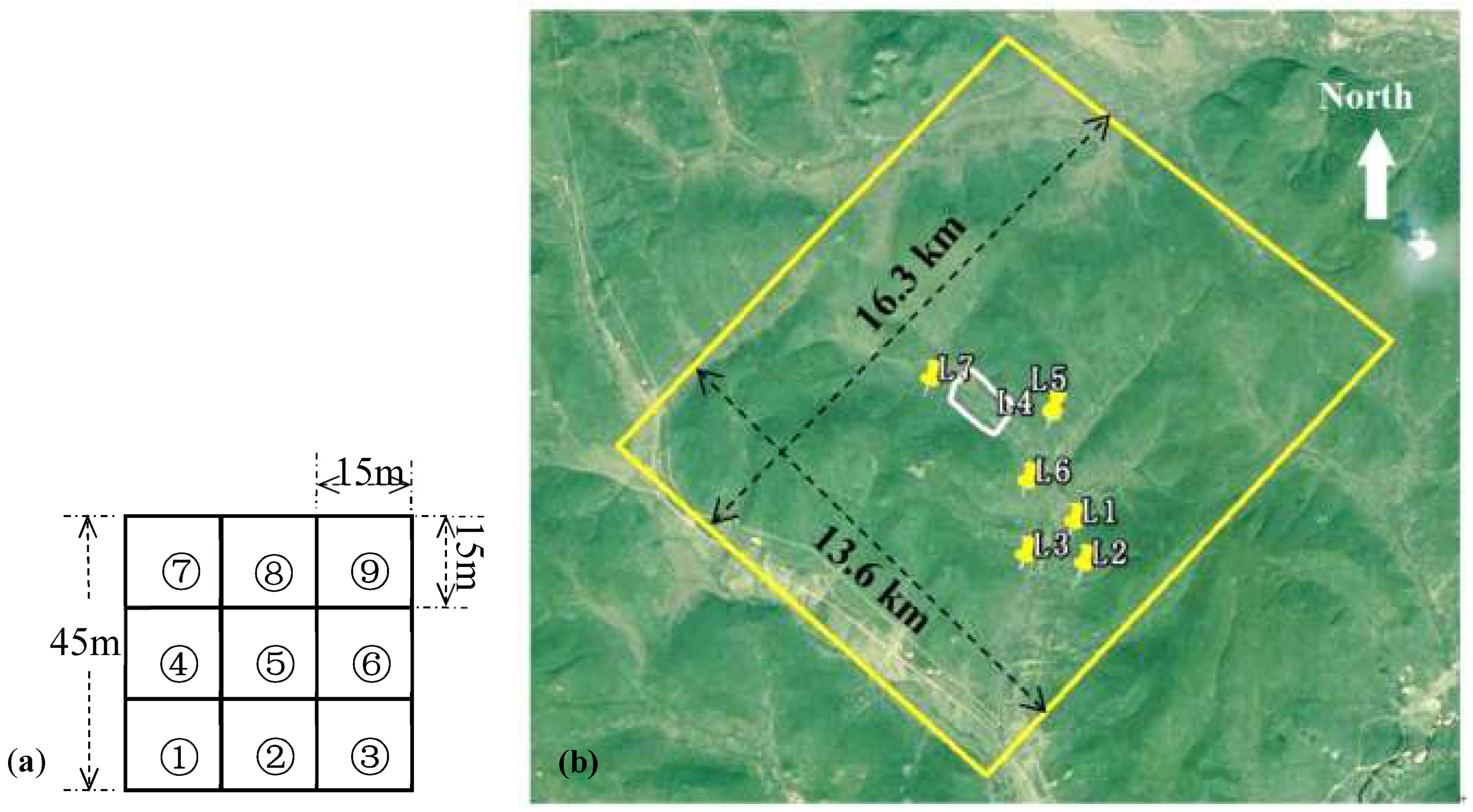
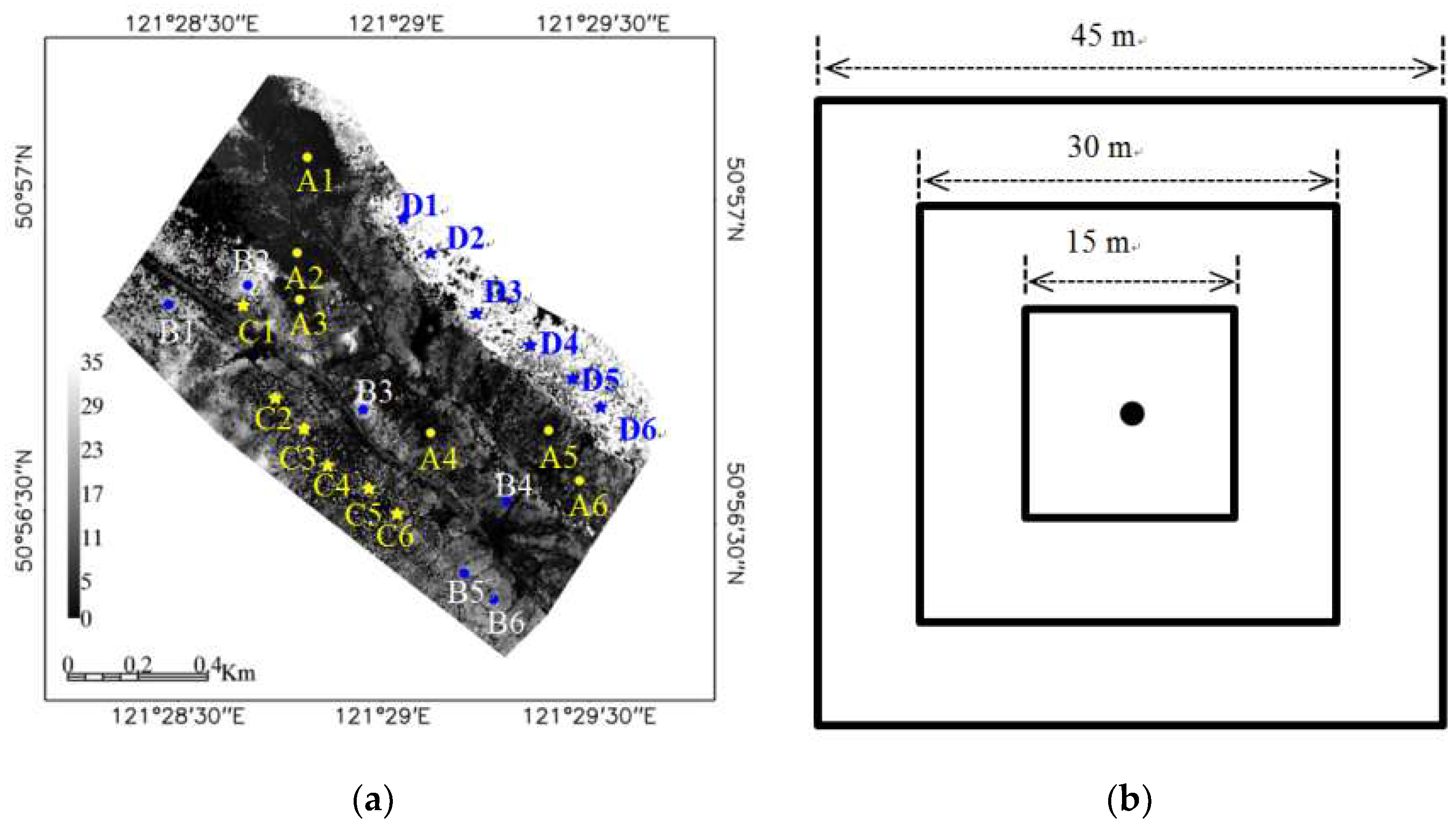
2.1. Test Sites

The study area is located at the Genhe forest bureau in the Inner Mongolia Autonomous Region of China (50°56′N, 121°29′E) on the northwest slope of Daxing’an Mountains. This area is on the southern border of boreal forest and belongs to the frigid-temperate zone of the coniferous forest vegetation. The elevation of this area ranges between 650 m–1269 m. The annual mean temperature is −5.4 °C, while the minimum temperature is −52.6 °C. This area is referred to as the cold polar of China. The annual mean precipitation is 450~550 mm, 60% of which occurs during July and August. The soil type is brown coniferous forest soil with a thickness of 30 cm~40 cm. 83.7% of the area is covered by forest. The dominant tree species is larch (Larix gmelinii). The main broadleaf deciduous species include white birch (Betula platyphlla) and aspen (populous davidiana). In the study area, the maximum height of the Dhurian larch is about 35 m and the maximum diameter at breast height (DBH) is about 40 cm.

2.2. Inventory of Ground Reference

The field sampling was carried out between 10 August and 15 August 2013 by a team under previous project using a plot size of 45 m × 45 m [34]. Each plot was divided into nine subplots with a size of 15 m × 15 m and subplots were numbered serially as shown in Figure 1a. The diameter at the breast height (DBH) of each tree was measured by DBH tape. The heights of the canopy tops and canopy bottoms of each tree were measured by laser range finder. The crown width of each tree at the directions of south to north and east to west were measured by taps. The positions of plot corners were measured by GPS with differential correction, while the relative position of each tree (with DBH > 5.0 cm) within the plots was measured by total stations. In total, seven plots were measured and there were two species of trees located within the plots, i.e. white birch and larch. The biomass of each tree was calculated using the measured DBH and tree heights and the published allometric equations, as shown in Table 1 [35]. The forest AGB of each subplot was the summation of aboveground biomass of all trees divided by the corresponding spatial area. The maximum, minimum, standard deviation, and average forest AGB of all subplots were 184.44 Mg/ha, 21.84 Mg/ha, 39.44 Mg/ha, 74.97 Mg/ha, respectively.

2.3. Forest AGB Maps from Lidar Data

The lidar system onboard Yun-5 aircraft was the Leica ALS60 (Leica Geosystems, Heerbrugg, Switzerland) system working at 1064 nm and a 166 kHz pulse rate at 1800 m above ground level (AGL). The Yun-5 aircraft carried both the GPS receivers and Inertial Navigation System (INS) simultaneously for recording accurate positions and attitudes of the platform. Three returns were recorded, i.e. first, second and last. The positioning accuracy was estimated as vertical error <15 cm and horizontal error <50 cm by comparing with the ground control points (GCPs) from Real Time Kinematic (RTK) measurements. The Lidar data used in this study was collected from 30 August to 14 September 2012 with a point density of about 2~4 points/m2. Please refer to [36] for more details on Lidar data acquisition.
The lidar point clouds were classified as ground, vegetation, and others using TerraScan software (TerraSolid Ltd, Helsinki, Finland, http://www.terrasolid.com/home.php) [37]. The DTM of the ground surface with a pixel size of 0.5 m was produced through the rasterization of the ALS ground points. The first return of the ALS point cloud was rasterized to produce a digital surface model (DSM) with a pixel size of 0.5m. If only one point was located within a pixel, the elevation of the point was used as the pixel value. If there were more than one point within a pixel, the mean height of vegetation points was used as the pixel value. The difference between DSM and DTM was the mean canopy height model (MCHM). The pixels with heights of <2.0 were set as 0.0 m to exclude shrubs and non-woody vegetation. The mean forest height of each plot was calculated by averaging all MCHM pixels, including both bare ground and vegetation pixels. The mean forest height of each subplot was correlated with the corresponding biomass density to build an estimation model of forest AGB. There were, in total, 63 subplots from 7 sampling plots. All subplots were numbered from 1 to 63 according to their serial number within each plot and the serial number of each plot. The 32 subplots with odd numbers were used to develop an estimation model of forest AGB and the rest of the 31 subplots were used for model validation. Considering that the forest AGB is linearly correlated with forest stocking volume, which is correlated with forest height in the power form as indicated in [38], the power function was chosen to develop an estimation model of forest AGB. Figure 2a shows that the determination coefficient (R2) between mean forest heights and field-measured forest AGB was 0.80, with a root mean square error (RMSE) of 24.4 Mg/ha, while Figure 2b shows that the R2 between field measurement and model predicted forest AGB of the validation plots was 0.74 with a RMSE of 16.9 Mg/ha. The MCHM map with a resolution of 15 m was produced in the same way as the calculation of the mean forest height of each plot. Then the forest AGB map produced using the developed model and MCHM, with a resolution of 15 m, is shown in Figure 2c.

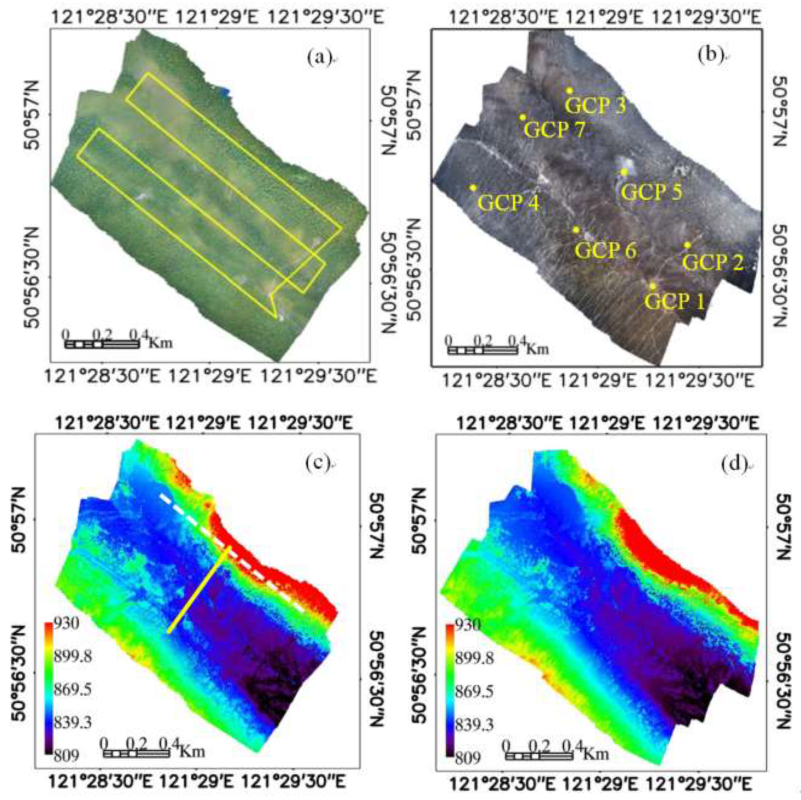
2.4. Collections of UAV Stereo Imagery

The acquisition system of stereo imagery was built on a six-rotor helicopter [27]. The camera mounted on the helicopter pointing at nadir was a Sony NEX-5T, which could collect images with 16.10 megapixels. The ground station associated with the UAV system enabled to automatically program the flying routes and the positions to take photos according to system settings, including focal lengths of camera, flying heights, forward overlaps, side overlaps, and flying speeds. The duration of each flight was determined by the battery capacity. Taking the battery of 16000 mAh used in this study for example, it was about 18–20 minutes flying at about 300 m AGL with a flying speed of 10 m/s. The forward overlap used in this study was about 90% while the side overlap was about 60%. The stereo imagery used in this study was collected by flying along the same routes on 25 August 2014 and 5 May 2015, corresponding to leaf-on and leaf-off seasons, respectively. The focal length and shutter speed used in image collection was 16 mm and 1/600 s, respectively. 776 images stored in the RGB format were used in this study. The spatial resolution or the ground sample distance (GSD) of the stereo imagery was about 8.6 cm.

2.5. Stereoscopic Processing

The stereo images were processed using the Agisoft Photoscan software package (version 1.2.2, build 2294, 64 bit). The processing algorithm was procedures of structure from motion (SfM). The three-dimensional modeling equations used in SfM only need relative positions and orientations of the camera, which can be calculated using identified matching points. The point cloud in local relative coordinate systems can be determined based on the numerous overlapping stereo images [39]. The real three-dimensional model was produced by transforming the relative point cloud into geo-referenced coordinates using GCP. Correspondingly, there were three basic steps involved in the stereo processing: (a) Image alignments, i.e. the relative positions and orientations of images were estimated using the key points extracted from images through analyses of image textures; (b) dense point cloud generation, i.e. based on the estimated relative positions and orientations of images—the depth information for each camera was calculated and then combined into a single dense point cloud. Five levels of quality of point densification are provided in the software, including lowest, low, medium, high, or ultra-high. The ultra-high level was used in this study to get the densest point cloud. (c) Coordinates transformation, i.e. the geo-referenced coordinates of point cloud was calculated from the relative coordinates using GCP. Three options were provided in step (b) to determine the filtering degree, including “mild,” “aggressive,” and “moderate.” For forested areas, the “mild” was recommended because the sparse single trees were always filtered out as noise by the other two settings. The default values of other parameters were used in this study.
The field measurement of GCP using GPS with differential correction was time-consuming in field work. The longitude, latitude, and elevation of GCPs used in this study were directly collected on the very height resolution (VHR) images in Google Earth™. The same GCPs were used for the stereo imagery of both leaf-on and leaf-off to minimize their divergence. The spatial distributions and the positioning errors of GCPs were shown in the results section.

3. Methods

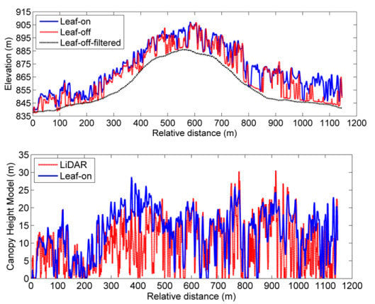
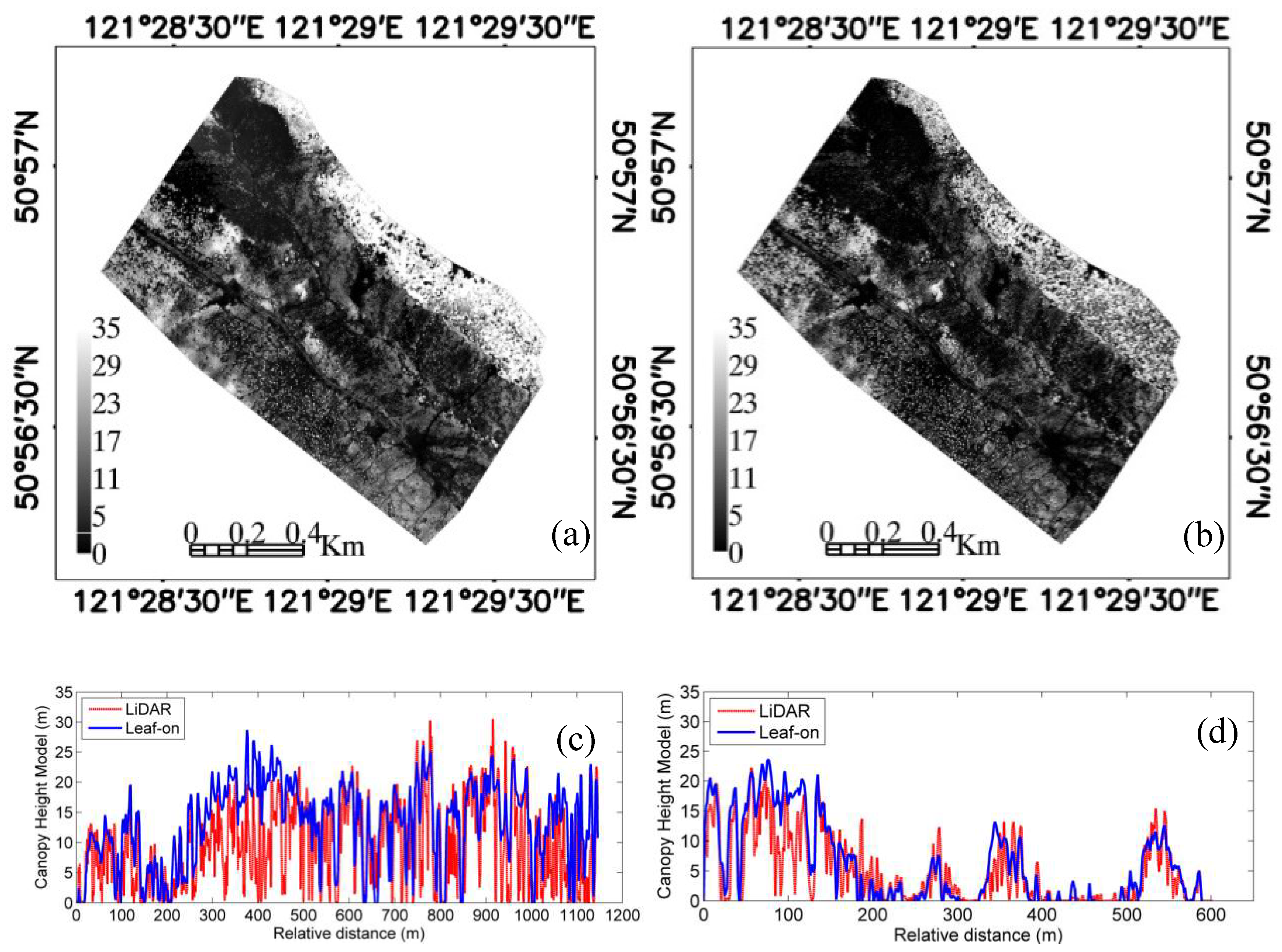
3.1. Extraction of Canopy Height Model

The direct results of the stereoscopic processing of images acquired in the leaf-off season are point clouds located on the vegetation and ground surfaces. The prerequisite of DTM extraction is to remove vegetation points. A simple automatic algorithm based on iterative median filtering (IMF) is used to identify ground points from the point cloud of the stereo imagery acquired on leaf-off season. The algorithm is described as follows:
(1) Point cloud is rasterized to produce an elevation image with a given pixel size, such as 5.0 m;
(2) The elevation image is filtered by median filter with a given window size, such as 13 × 13;
(3) The filtered elevation image serves as a template to screen out point cloud; points above the template are discarded if their vertical distance to the template is larger than a given threshold, such as 1.5 m;
(4) the remained point cloud is processed by repeating steps (1)–(3) until the number of discard points is smaller than a given threshold, such as 1%.
The DSM of the forest canopy top could be generated by rasterizing the point cloud of leaf-on with a resolution of 0.5 m in the same way as the rasterization of lidar point cloud. The DTM could be produced by the rasterization and interpolation of the filtered point cloud of leaf-off. Therefore, the MCHM could be extracted by subtracting DTM from DSM.

3.2. Mapping of Forest AGB Using MCHM of UAV Stereo Imagery

Considering the fact that the UAV stereo imagery should be available before the field work of tree measurements, this study proposed to determine positions of field sampling plots on the MCHM of UAV stereo imagery and ortho-rectified mosaic images, because they can provide information about the spatial distribution of forest canopy heights, forest densities, tree species and so on. For the coverage of as full a dynamic range of forest AGB as we can, four types of sampling plots were selected, including low and sparse forests (referred to as type A), low and dense forests (referred to as type B), two-layer forests with sparse higher trees (referred to as type C) and high and dense forests (referred to as type D). Six field sampling plots were selected for each type.
The time-cost of field measurements for each plot is directly determined by the size of sampling plots. More time is needed for a larger sampling plot because more trees located within plots should be measured. What is the proper size of sampling plots of the field measurements for the mapping of forest AGB using UAV stereo imagery? In order to answer this question, considering the plot size of field measurement used in this study as in Section 2.2, three sizes of sampling plots were used in this study, i.e. concentric square plots with sizes of 15 m × 15 m, 30 m × 30 m and 45 m × 45 m.
The field sampling plots described in Section 2.2 were not located within the coverage of UAV stereo imagery, as show in Figure 1b. Therefore, the values of forest AGB of sampling plots had to be collected from the forest AGB map of lidar produced in the Section 2.3. For 15 m × 15 m plots, the value of forest AGB can be directly collected from the forest AGB map of lidar. For 30 m × 30 m (or 45 m × 45 m) plots, the average of all four (or nine) pixels in forest AGB map of lidar covered by the sampling plot are used as a sampling of forest AGB in the model development. The prediction models were developed by taking the mean pixel values of MCHM of stereo imagery and the forest AGB of sampling plots as explanatory and response variables, respectively. The three MCHM maps with the spatial resolutions of 15 m × 15 m, 30 m × 30 m and 45 m × 45 m were produced using the UAV MCHM with a resolution of 0.5 m in the same as the producing of lidar MCHM maps. The three forest AGB maps of UAV stereo imagery were further generated using the UAV MCHM maps and the corresponding prediction models. The three forest AGB maps of UAV stereo imagery were evaluated by taking that of lidar data as reference. The evaluation was carried out using the pixel by pixel comparison between the forest AGB maps of UAV and those of lidar.

4. Results

4.1. UAV Stereo Imagery

Figure 3 showed the ortho-rectified mosaic images and DSM of UAV stereo imagery acquired in leaf-on and leaf-off seasons over the test site. The reported density of point cloud extracted from the UAV stereo imagery of leaf-on and leaf-off was 32.4 point/m2 and 35.9 point/m2, respectively. The UAV trajectory was overlaid on Figure 3a showed as yellow lines. The coverage area was about 1.52 km2 with a 1.6 km length and 0.95 km width. Both the leaf-on and leaf-off stereo imagery were collected along the same trajectory within one flight with an effective duration of flight of about 12 minutes. One obvious difference between leaf-on and leaf-off was that more roads were visible in Figure 3b than in Figure 3a. There were no harvesting activities that occurred between the two flights, but the snow covered the ground, and the leaves were off during the collection of early spring images.
The accuracy of GCP was shown in Table 2. The standard deviation of GCP in leaf-off season along the direction from west to east was 0.59 m, while that along the direction from south to north was 0.48 m. The vertical accuracy was 0.8 m. For GCP in leaf-on season, the vertical accuracy was 0.83 m, while the horizontal accuracy was 0.34 m and 0.32 m along the direction from west to east and the direction from south to north, respectively.
The accuracy of GCP reported in Table 1 indicated the relative co-registration errors between the UAV imagery of Leaf-on and Leaf-off. The absolution positioning error is evaluated by making an accurate co-registration between the DSM of Leaf-on and that of lidar using the method proposed in [40]. The results show that the horizontal offset between the two DSM is about 3.63 pixel (3.63 pixel * 0.5 m/pixel = 1.815 m) and 0.67 pixel (0.67 pixel * 0.5 m/pixel = 0.335 m) along the X and Y directions, respectively. For the field plot with a size of 15 m × 15m or even larger, the positioning error was only about 1/10 of plot size, which is acceptable.

4.2. Extraction of Forest Canopy Heights

Figure 4 shows the results of the extraction of ground surfaces using leaf-off stereo imagery by the IMF at different aspects. The number and percentage of points removed in each iteration is shown in Figure 4a. It is clear that the vegetation points are mostly removed in the first two iterations. The number of removed points decreased gradually after each iteration and was lower than 1% after the fifth iteration. Figure 4b shows the identification of ground points along a profile over flat terrain conditions. The profile is a subset of the point cloud along the X direction (from west to east) with a length of 115 m. It could be seen that the identified points gradually approached the ground surface. The difference between iterations becomes very weak after the third iteration. Figure 4c depicts the vertical distribution of points over a forest stand of 30 m × 30 m. The vertical distribution of the remaining points concentrates gradually on the ground surface. Figure 4 showed that the elevation of ground surface can be extracted well by the IMF algorithm in both flat and mountainous areas.
The MCHM extracted by the synergy of point cloud of leaf-on stereo imagery and the filtered point cloud of leaf-off stereo imagery is shown in Figure 5. Figure 5a,b are the leaf-on UAV MCHM and lidar MCHM, respectively. The two images look nearly identical at a first glance. These results demonstrated that the elevation of ground surface extracted from the point cloud of leaf-off stereo imagery by IMF was enough. In addition, the point cloud of leaf-on stereo imagery and leaf-off stereo imagery has been co-registered accurately enough by the GCPs; otherwise, there would be terrain-related errors remained in Figure 5a caused by their mis-registration.
The comparison between the leaf-on UAV MCHM and lidar MCHM is shown in Figure 5c,d along two profiles which are identical to Figure 4d,e respectively. The changing trends of forest heights along profiles of leaf-on UAV MCHM and lidar MCHM were consistent. The pixels where the leaf-on UAV MCHM was higher than the lidar MCHM could be attributed to the bad penetration abilities of stereo imagery over higher tree neighboring those pixels. The pixels where the leaf-on UAV MCHM was lower than lidar MCHM were caused by a failure to catch the canopy tops of trees neighboring those pixels.

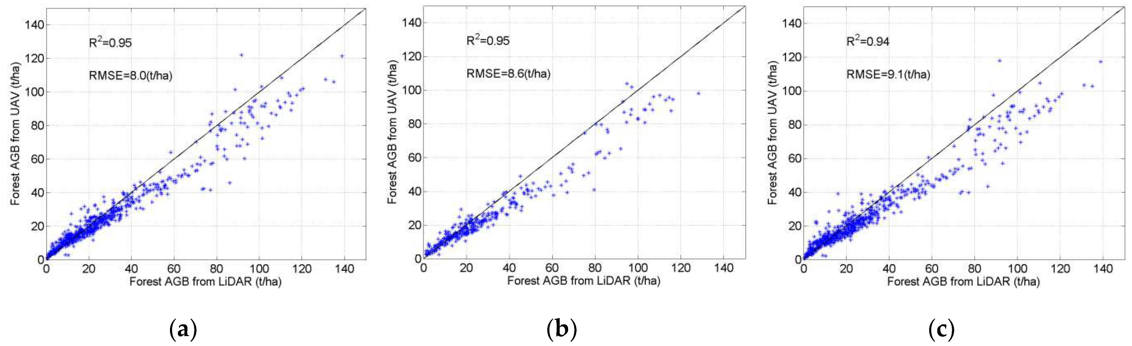
4.3. Model Development and Validation of Forest AGB Maps of UAV

The positions of 24 sampling plots are shown in Figure 6a. The symbols of yellow dots, blue dots, yellow stars, and blue stars represent the sampling plots of type A, type B, type C, and type D, respectively. Three concentric square plots with different sizes as shown in Figure 6b are setup at each position to evaluate the effects of plot size on the accuracy of prediction models based on UAV stereo imagery. The MCHM images of four 45 m × 45 m sampling plots representing four stand categories are shown in Figure 7. Figure 7a to Figure 7d are the MCHM of the UAV stereo imagery with a resolution of 0.5 m corresponding to the sampling plots of A1, B1, C1, and D1. Figure 7e to Figure 7h are the vertical distribution of points corresponding to Figure 7a to Figure 7d.
The prediction models of forest AGB using mean forest heights from UAV stereo imagery take the form of power functions as that of lidar. The model coefficients and accuracy are shown in Table 3. The scattering plot of the forest AGB from lidar against that predicted by the prediction models is given in Figure 8. Both Table 3 and Figure 8 show that the differences of prediction accuracy from the models developed at different plot sizes are not obvious in terms of R2. The accuracy differences in terms of RMSE are also weak, which is about 1.8 Mg/ha between 15 m × 15 m and 30 m × 30 m, and 1.4Mg/ha between 30 m × 30 m and 45 m × 45 m. Figure 9 shows that the forest AGB of sampling plots scattered evenly among the dynamic range from 0 to 140 Mg/ha. The results show that the dynamic range of forest AGB can be covered by sampling plots selected on MCHM of UAV and ortho-rectified mosaic image.
Three maps of forest AGB from UAV are produced by the three prediction models developed at sampling plot sizes of 15 m × 15 m, 30 m × 30 m and 45 m × 45 m. Figure 9 shows the validation of forest AGB maps by taking those of lidar as a reference. The three forest AGB maps of the UAV stereo images are highly correlated with those of the lidar data with correlation coefficients (R2) larger than 0.94 and the root mean square errors (RMSEs) are smaller than 10 Mg/ha. No obvious differences or trends of the estimation accuracy of forest AGB are observed along with the changes of sampling plot sizes. The results indicate that the field sampling plots with a size of 15 m × 15 m are large enough, at least over the research area of this study, for the mapping of forest AGB using UAV stereo imagery.

5. Discussions

5.1. Extraction of Ground Surface

Four parameters are needed in the proposed IMF algorithm, i.e. the pixel size used in the rasterization of point cloud, the window size used in median filtering, the threshold of vertical distance to the template, and the number of iterations. The requirement for pixel size is not rigorous. The ranges from 1.0 m to 10.0 m are acceptable for stereo imagery with a resolution smaller than 0.1 m, as used in this study. There will be no sufficient number of points for the interpolation if the pixel size is too small, while the small terrain features will be missed if the pixel size is too large.
The IMF algorithm is also not sensitive to the filtering window size. The ranges from 3 × 3 to 15 × 15 are all acceptable. The difference between different window sizes is the work efficiency. More iterations are needed for smaller window sizes because most features of forests’ vertical structures are retained. A filtering widow size that is too large is not suggested because detailed terrain features will be missed, as in the case of the large pixel size used in the rasterization.
The threshold of vertical distance to the template is a critical parameter of IMF because points having a vertical distance larger than the threshold are directly discarded. The larger threshold will slow down the filtering process while a smaller threshold will remove the point of the ground surface on the slope. The minimum of the threshold should be the integrated consideration of terrain slopes, pixel size, and filtering window size to guarantee that the threshold is larger than the elevation fluctuation of ground surfaces. In this study, the fixed threshold was used because the elevation dynamics over the coverage area are narrow. In future studies, it would be worthwhile to adjust the threshold adaptively for application over larger areas with broader dynamics of ground surface elevations.
The last parameter of IMF is the number of iterations. The results in this study showed that the filtering should be stopped when the number of points removed is lower than 1% of the original point number. This parameter, in fact, is not particularly important because the intermediate results can be saved in the filtering process. Users can determine which one is the best result by comparing these intermediate results.

5.2. The applicable Areas of UAV Stereo Imagery

The applicable area of this study is limited to deciduous forests. This limitation is mainly due to the availability of ground surface elevations under forest canopies because the leaf-off conditions increase the probability to see through the forest canopies over the deciduous forest. In fact, the description of forest spatial structures mainly comes from the UAV stereo imagery of leaf-on. The UAV stereo imagery is anticipated to also have good performance over evergreen forest areas if a high quality elevation dataset of the ground surface under the forest canopy is available or over sparse forest areas like savanna or forest shelterbelts.

5.3. Uncertainties

It must be noted that some kinds of uncertainties existed in this study. The most obvious uncertainty is the mis-match of acquisition dates of data used in this study. The lidar data was collected in 2012, the field measurements were carried out in 2013, and the UAV stereo imagery was collected in 2014 and 2015. Considering that the forest structure is, in fact, derived from leaf-on stereo imagery, the time interval between lidar and UAV stereo imagery is about two years. No obvious or severe human disturbances occurred in these two year. The forest growth is slow because the growing season of this area is only about four months from late May to early September. It could be anticipated that the correlation between forest biomass from lidar and that from UAV stereo imagery might be improved or at least might not be decreased if these two datasets were acquired in the same period.
Another uncertainty is the different point density. The point density of lidar data is about 2 ~ 4 points/m2 while that of the UAV stereo imagery is higher than 30 points/m2. The holes within forest canopies can be observed on the DSM of the lidar data, with a resolution of 0.5 m. The point cloud of UAV stereo imagery was rasterized into the DSM with a resolution of 0.5 m to reduce the uncertainty of unmatched point densities.
In this study, the forest AGB measurements for the developments of prediction models of UAV stereo imagery was collected on the forest AGB maps of lidar data, due to the unavailability of field measurements within the coverage of UAV stereo imagery. Although the analysis was carried out on the forest AGB, the comparison was in fact equivalently made on the vertical forest structures detected by UAV stereo imagery and those detected by lidar data. The uncertainties, exhibited on fine resolutions such as 15 m × 15 m, as shown in Figure 9, could be attributed to their different performances of the detection of forest vertical structures. For example, the small gaps between crowns could be seen by lidar data but missed by UAV stereo imagery, as shown in Figure 5c,d. Inversely, the lidar data was easily affected by the gaps within crowns, while the UAV stereo imagery could describe crowns with good geometrical shapes by overpassing those gaps within crowns. In future studies, the UAV stereo imagery should be further evaluated against the field measurements of trees.

6. Conclusion

The application of UAV stereo imagery as a practical sampling tool of forests is limited by the ground surface elevation under the forest canopy. Most studies on the extraction of forest spatial structures using UAV stereo imagery used the DTM from lidar data. Therefore, they are mostly limited within the area where the lidar DTM is available. In this study, we proposed a new way to extract the deciduous forest canopy height without the help of the lidar DTM. The central idea is that the synthesis of UAV stereo imagery acquired under leaf-on and leaf-off condition. The point cloud derived from the leaf-off UAV stereo imagery was firstly processed by the proposed algorithm of iterative median filtering to remove points from forests. The digital terrain model (DTM) was produced by the rasterization of filtered point cloud. The digital surface model (DSM) of the forest canopy top was generated by rasterizing the point cloud derived from the leaf-on UAV stereo imagery. The mean forest canopy height model (MCHM) was derived from the DSM subtracted by the DTM. The results showed that the terrain information in the DSM could be removed in the MCHM.
The extracted MCHM was further used for the mapping of forest AGB. Results showed that forest AGB maps from UAV stereo imagery were highly correlated with those from the lidar data with R2 higher than 0.94 and RMSE lower than 10.0 Mg/ha. The underestimation of AGB by UAV data was observed. The reason for this underestimation should be explored over more test sites in the future.

Author Contributions

Conceptualization, W.N.; methodology, W.N. and J.D.; software, J.D.; validation, W.N., Y.P. and X.T.; formal analysis, W.N.; investigation, W.N.; resources, Z.Z.; data curation, W.N.; writing—original draft preparation, W.N.; writing—review and editing, G.S.; visualization, W.N. and J.D.; project administration, E.C.; funding acquisition, Z.L.

Funding

This work was funded in part by the National Key R&D Program of China under Grant 2017YFA0603002, National Basic Research Program of China (Grant No. 2013CB733404, 2013CB733401), and in part by the National Natural Science Foundation of China (Grant Nos. 41471311, 41371357, 41301395).

Acknowledgments

Special thanks to the forest field inventory team members for the valuable field inventory data including Qiang Wang, Li Zhao, Xiyun Mu, Kan Huang, Chunmei Li, Da Huo, Changlong Li, Bin Sun, Lu Wang, Yun Guo, Yu Zhang, Xiaohong Li, Chong Ren, Min Yan, Lan Li, Wangfei Zhang, Kailong Hu and Hui Song.

Conflicts of Interest

The authors declare no conflict of interest.

References

  1. Kindermann, G.E.; Mcallum, I.; Fritz, S.; Obersteiner, M. A global forest growing stock, biomass and carbon map based on FAO statistics. Silva Fenn. 2008, 42, 387–396. [Google Scholar] [CrossRef]
  2. Pan, Y.D.; Birdsey, R.A.; Fang, J.Y.; Houghton, R.; Kauppi, P.E.; Kurz, W.A.; Phillips, O.L.; Shvidenko, A.; Lewis, S.L.; Canadell, J.G.; et al. A Large and Persistent Carbon Sink in the World’s Forests. Science 2011, 333, 988–993. [Google Scholar] [CrossRef] [PubMed]
  3. Beer, C.; Reichstein, M.; Tomelleri, E.; Ciais, P.; Jung, M.; Carvalhais, N.; Rodenbeck, C.; Arain, M.A.; Baldocchi, D.; Bonan, G.B.; et al. Terrestrial Gross Carbon Dioxide Uptake: Global Distribution and Covariation with Climate. Science 2010, 329, 834–838. [Google Scholar] [CrossRef]
  4. Rosenqvist, A.; Shimada, M.; Ito, N.; Watanabe, M. ALOS PALSAR: A Pathfinder mission for global-scale monitoring of the environment. IEEE Trans. Geosci. Remote Sens. 2007, 45, 3307–3316. [Google Scholar] [CrossRef]
  5. Rosenqvist, A.; Shimada, M.; Suzuki, S.; Ohgushi, F.; Tadono, T.; Watanabe, M.; Tsuzuku, K.; Watanabe, T.; Kamijo, S.; Aoki, E. Operational performance of the ALOS global systematic acquisition strategy and observation plans for ALOS-2 PALSAR-2. Remote Sens. Environ. 2014, 155, 3–12. [Google Scholar] [CrossRef]
  6. Le Toan, T.; Quegan, S.; Davidson, M.W.J.; Balzter, H.; Paillou, P.; Papathanassiou, K.; Plummer, S.; Rocca, F.; Saatchi, S.; Shugart, H.; et al. The BIOMASS mission: Mapping global forest biomass to better understand the terrestrial carbon cycle. Remote Sens. Environ. 2011, 115, 2850–2860. [Google Scholar] [CrossRef] [Green Version]
  7. Lefsky, M.A. A global forest canopy height map from the Moderate Resolution Imaging Spectroradiometer and the Geoscience Laser Altimeter System. Geophys. Res. Lett. 2010, 37, L15401. [Google Scholar] [CrossRef]
  8. Baccini, A.; Goetz, S.J.; Walker, W.S.; Laporte, N.T.; Sun, M.; Sulla-Menashe, D.; Hackler, J.; Beck, P.S.A.; Dubayah, R.; Friedl, M.A.; et al. Estimated carbon dioxide emissions from tropical deforestation improved by carbon-density maps. Nat. Clim. Chang. 2012, 2, 182–185. [Google Scholar] [CrossRef]
  9. Simard, M.; Pinto, N.; Fisher, J.B.; Baccini, A. Mapping forest canopy height globally with spaceborne lidar. J. Geophys. Res. Biogeosci. 2011, 116, G04021. [Google Scholar] [CrossRef]
  10. Blackard, J.A.; Finco, M.V.; Helmer, E.H.; Holden, G.R.; Hoppus, M.L.; Jacobs, D.M.; Lister, A.J.; Moisen, G.G.; Nelson, M.D.; Riemann, R.; et al. Mapping US forest biomass using nationwide forest inventory data and moderate resolution information. Remote Sens. Environ. 2008, 112, 1658–1677. [Google Scholar] [CrossRef]
  11. Saatchi, S.S.; Harris, N.L.; Brown, S.; Lefsky, M.; Mitchard, E.T.A.; Salas, W.; Zutta, B.R.; Buermann, W.; Lewis, S.L.; Hagen, S.; et al. Benchmark map of forest carbon stocks in tropical regions across three continents. Proc. Natl. Acad. Sci. USA 2011, 108, 9899–9904. [Google Scholar] [CrossRef] [PubMed] [Green Version]
  12. Rodríguez-Veiga, P.; Saatchi, S.; Tansey, K.; Balzter, H. Magnitude, spatial distribution and uncertainty of forest biomass stocks in Mexico. Remote Sens. Environ. 2016, 183, 265–281. [Google Scholar] [CrossRef] [Green Version]
  13. Hall, F.G.; Bergen, K.; Blair, J.B.; Dubayah, R.; Houghton, R.; Hurtt, G.; Kellndorfer, J.; Lefsky, M.; Ranson, J.; Saatchi, S.; et al. Characterizing 3D vegetation structure from space: Mission requirements. Remote Sens. Environ. 2011, 115, 2753–2775. [Google Scholar] [CrossRef] [Green Version]
  14. Gonzalez, P.; Asner, G.P.; Battles, J.J.; Lefsky, M.A.; Waring, K.M.; Palace, M. Forest carbon densities and uncertainties from Lidar, QuickBird, and field measurements in California. Remote Sens. Environ. 2010, 114, 1561–1575. [Google Scholar] [CrossRef]
  15. Montesano, P.M.; Nelson, R.F.; Dubayah, R.O.; Sun, G.; Cook, B.D.; Ranson, K.J.R.; Raesset, E.N.; Kharuk, V. The uncertainty of biomass estimates from LiDAR and SAR across a boreal forest structure gradient. Remote Sens. Environ. 2014, 154, 398–407. [Google Scholar] [CrossRef]
  16. Lu, D.S.; Chen, Q.; Wang, G.X.; Liu, L.J.; Li, G.Y.; Moran, E. A survey of remote sensing-based aboveground biomass estimation methods in forest ecosystems. Int. J. Digit. Earth 2016, 9, 63–105. [Google Scholar] [CrossRef]
  17. Avitabile, V.; Herold, M.; Henry, M.; Schmullius, C. Mapping biomass with remote sensing: A comparison of methods for the case study of Uganda. Carbon Balance Manag. 2011, 6, 7. [Google Scholar] [CrossRef]
  18. Keller, M.; Palace, M.; Hurtt, G. Biomass estimation in the Tapajos National Forest, Brazil—Examination of sampling and allometric uncertainties. For. Ecol. Manag. 2001, 154, 371–382. [Google Scholar] [CrossRef]
  19. Chave, J.; Condit, R.; Aguilar, S.; Hernandez, A.; Lao, S.; Perez, R. Error propagation and scaling for tropical forest biomass estimates. Philos. Trans. R. Soc. Lond. Ser. B-Biol. Sci. 2004, 359, 409–420. [Google Scholar] [CrossRef]
  20. Mascaro, J.; Detto, M.; Asner, G.P.; Muller-Landau, H.C. Evaluating uncertainty in mapping forest carbon with airborne LiDAR. Remote Sens. Environ. 2011, 115, 3770–3774. [Google Scholar] [CrossRef] [Green Version]
  21. Ferraz, A.; Saatchi, S.; Mallet, C.; Meyer, V. Lidar detection of individual tree size in tropical forests. Remote Sens. Environ. 2016, 183, 318–333. [Google Scholar] [CrossRef]
  22. Wallace, L.; Lucieer, A.; Watson, C.; Turner, D. Development of a UAV-LiDAR System with Application to Forest Inventory. Remote Sens. 2012, 4, 1519–1543. [Google Scholar] [CrossRef] [Green Version]
  23. Getzin, S.; Nuske, R.S.; Wiegand, K. Using Unmanned Aerial Vehicles (UAV) to Quantify Spatial Gap Patterns in Forests. Remote Sens. 2014, 6, 6988–7004. [Google Scholar] [CrossRef] [Green Version]
  24. Zarco-Tejada, P.J.; Diaz-Varela, R.; Angileri, V.; Loudjani, P. Tree height quantification using very high resolution imagery acquired from an unmanned aerial vehicle (UAV) and automatic 3D photo-reconstruction methods. Eur. J. Agron. 2014, 55, 89–99. [Google Scholar] [CrossRef] [Green Version]
  25. Dandois, J.; Olano, M.; Ellis, E. Optimal Altitude, Overlap, and Weather Conditions for Computer Vision UAV Estimates of Forest Structure. Remote Sens. 2015, 7, 13895. [Google Scholar] [CrossRef]
  26. Dandois, J.P.; Ellis, E.C. High spatial resolution three-dimensional mapping of vegetation spectral dynamics using computer vision. Remote Sens. Environ. 2013, 136, 259–276. [Google Scholar] [CrossRef] [Green Version]
  27. Ni, W.; Liu, J.; Zhang, Z.; Sun, G.; Yang, A. Evaluation of UAV-based forest inventory system compared with LiDAR data. In Proceedings of the 2015 IEEE International Geoscience and Remote Sensing Symposium (IGARSS), Milan, Italy, 26–31 July 2015. [Google Scholar]
  28. St-Onge, B.; Vega, C.; Fournier, R.A.; Hu, Y. Mapping canopy height using a combination of digital stereo-photogrammetry and lidar. Int. J. Remote Sens. 2008, 29, 3343–3364. [Google Scholar] [CrossRef]
  29. Persson, H.; Wallerman, J.; Olsson, H.; Fransson, J.E.S. Estimating forest biomass and height using optical stereo satellite data and a DTM from laser scanning data. Can. J. Remote Sens. 2013, 39, 251–262. [Google Scholar] [CrossRef]
  30. Hobi, M.L.; Ginzler, C. Accuracy Assessment of Digital Surface Models Based on WorldView-2 and ADS80 Stereo Remote Sensing Data. Sensors 2012, 12, 6347–6368. [Google Scholar] [CrossRef] [Green Version]
  31. Ni, W.; Sun, G.; Ranson, K.J.; Pang, Y.; Zhang, Z.; Yao, W. Extraction of ground surface elevation from ZY-3 winter stereo imagery over deciduous forested areas. Remote Sens. Environ. 2015, 159, 194–202. [Google Scholar] [CrossRef]
  32. Ni, W.; Sun, G.; Pang, Y.; Zhang, Z.; Liu, J.; Yang, A.; Wang, Y.; Zhang, D. Mapping Three-Dimensional Structures of Forest Canopy Using UAV Stereo Imagery: Evaluating Impacts of Forward Overlaps and Image Resolutions With LiDAR Data as Reference. IEEE J. Sel. Top. Appl. Earth Obs. Remote Sens. 2018, 11, 3578–3589. [Google Scholar] [CrossRef]
  33. Zhang, D.; Liu, J.; Ni, W.; Sun, G.; Zhang, Z.; Liu, Q.; Wang, Q. Estimation of Forest Leaf Area Index Using Height and Canopy Cover Information Extracted From Unmanned Aerial Vehicle Stereo Imagery. IEEE J. Sel. Top. Appl. Earth Obs. Remote Sens. 2019, 1–11. [Google Scholar] [CrossRef]
  34. Tian, X.; Li, Z.; Chen, E.; Liu, Q.; Yan, G.; Wang, J.; Niu, Z.; Zhao, S.; Li, X.; Pang, Y.; et al. The Complicate Observations and Multi-Parameter Land Information Constructions on Allied Telemetry Experiment (COMPLICATE). PLoS ONE 2015, 10, e0137545. [Google Scholar] [CrossRef]
  35. State Forestry Administration, P.R. China, SFAC. Guidelines on Carbon Accounting and Monitoring for Afforestation Project. 2011. Available online: https://wenku.baidu.com/view/4e27d5313968011ca 300911f.html (accessed on 11 April 2019).
  36. Pang, Y.; Li, Z.; Zhao, K.; Chen, E.; Sun, G. Temperate forest aboveground biomass estimation by means of multi-sensor fusion: The Daxinganling campaign. In Proceedings of the International symposium of Geoscience and Remote Sensing Society, Melbourne, Australia, 21–26 July 2013; pp. 991–994. [Google Scholar]
  37. Li, W.K.; Guo, Q.H.; Jakubowski, M.K.; Kelly, M. A New Method for Segmenting Individual Trees from the Lidar Point Cloud. Photogramm. Eng. Remote Sens. 2012, 78, 75–84. [Google Scholar] [CrossRef]
  38. Urban, D.L. A Versatile Model to Simulate Forest Pattern: A User’s Guide to ZELIG, version 1.0; University of Virginia: Charlottesville, VA, USA, 1990. [Google Scholar]
  39. Snavely, N.; Seitz, S.M.; Szeliski, R. Modeling the world from Internet photo collections. Int. J. Comput. Vis. 2008, 80, 189–210. [Google Scholar] [CrossRef]
  40. Ni, W.; Sun, G.; Zhang, Z.; Guo, Z.; He, Y. Co-registration of Two DEMs: Impacts on Forest Height Estimation from SRTM and NED at Mountainous Areas. IEEE Geosci. Remote Sens. Lett. 2014, 11, 273–277. [Google Scholar] [CrossRef]
Figure 1. The shape and spatial distribution of field sampling plots within the coverage of lidar data. The background true color image was from GoogleEarthTM. (a) the shape and size of field sampling plots; (b) the spatial distribution of field sampling plots, the white polygon was the area covered by Unmanned Aerial Vehicle (UAV) stereo imagery.
Remotesensing 11 00889 g001
Figure 2. Generation of forest aboveground biomass (AGB) reference using Lidar data. (a) Model development (32 plots); (b) model validation (31 plots); (c) forest AGB map with a resolution of 15 m from lidar data.
Remotesensing 11 00889 g002
Figure 3. Ortho-rectified mosaic images and digital surface model (DSM) of UAV stereo imagery acquired in leaf-on and leaf-off conditions (pixel size 8.6 cm). (a) the mosaic image of leaf-on with the flying trajectory showed as yellow lines; (b) the mosaic image of leaf-off with ground control points (GCPs) used in the stereoscopic processing showed as yellow dots; (c) the digital surface model of stereo imagery acquired on leaf-on season, the dash and solid lines indicates positions of two profiles used in the following sections; (d) the digital surface model of stereo imagery acquired on leaf-off season;.
Remotesensing 11 00889 g003
Figure 4. Elevation of ground surfaces extracted from the point cloud of UAV stereo imagery of leaf-off filtered by the method of iterative median filter (IMF). (a) The number and percentage of point removed at each iteration; (b) the results of each iteration along a vertical profile; (c) the results of each iteration over a 30 m × 30 m plot; (d) profiles along the white dash line in Figure 3c with an approximate length of 1150 m; (e) the profiles along the yellow solid line in Figure 3c with an approximate length of 600 m.
Remotesensing 11 00889 g004
Figure 5. Forest spatial structures extracted by the synergy of point cloud of leaf-on stereo imagery and the filtered point cloud of leaf-off stereo imagery. (a) leaf-on UAV mean canopy height model (MCHM), i.e., MCHM extracted from point cloud of leaf-on stereo imagery subtracted by the digital terrain model (DTM) produced by IMF; (b) lidar MCHM, the MCHM from lidar data; (c) profiles of leaf-on UAV MCHM and lidar MCHM along the same line as Figure 4d; (d) profiles of leaf-on UAV MCHM and lidar MCHM along the same line as Figure 4e.
Remotesensing 11 00889 g005
Figure 6. The sampling plots of forest AGB used for model developments. (a) the spatial distributions of sampling plots, type A: yellow dots, type B: blue dots, type C: yellow stars, type D: blue stars; the background image was the same as Figure 6a; (b) the relative positions of sampling plots with different sizes.
Remotesensing 11 00889 g006
Figure 7. The MCHM of 45 m × 45 m field sampling plots. (ad) were the MCHM of UAV stereo imagery with a resolution of 0.5 m corresponding to the sampling plots of A1, B1, C1, and D1. (eh) were the vertical distribution of points corresponding to (ad).
Remotesensing 11 00889 g007
Figure 8. Comparisons of forest AGB estimated from lidar and UAV stereo data using models developed at different plot sizes (24 plots for each plot size, i.e. 4 types ×6 plots/types). RMSE, root mean square error.
Remotesensing 11 00889 g008
Figure 9. Validation of forest AGB maps taking those from lidar as references (574 points). Points (ac) are the results using forest AGB maps from the predictions model developed on sampling plots of size 15 m × 15 m, 30 m × 30 m and 45 m × 45 m, respectively.
Remotesensing 11 00889 g009
Table 1. Allometric equations used in this study.
SpeciesAllometric Equations *
white birch Wt = 0.1193 ( D B H 2 H ) 0.8372
larch Ws = 0.04607 ( D B H 2 H ) 0.8722
Wb = 0.0356 ( D B H 2 H ) 0.5624
Wl = 0.01397 ( D B H 2 H ) 0.5628
Wt = Ws + Wb +   Wl
* Wt, Ws, Wb, Wl are biomass of total, stem, branch, and leaves respectively.
Table 2. Accuracy of the GCP in the stereoscopic processing of UAV stereo imagery (in meter).
GCP#X ErrorY ErrorZ ErrorGCP#X ErrorY ErrorZ Error
leaf-off p10.050.24−0.98leaf-on p1−0.13−0.23−1.11
leaf-off p20.26−0.900.90leaf-on p20.20−0.350.96
leaf-off p30.08−0.180.34leaf-on p3−0.34−0.130.48
leaf-off p40.800.44−0.08leaf-on p40.670.220.37
leaf-off p5−0.010.38−0.92leaf-on p5−0.130.60−0.54
leaf-off p60.010.291.0leaf-on p6−0.02−0.130.72
leaf-off p7−1.18−0.28−0.27leaf-on p7−0.260.01−0.87
Standard deviation0.590.480.80Standard deviation0.340.320.83
Table 3. Prediction models of forest AGB using a mean forest height of UAV stereo imagery at different plot sizes, taking the form of y = ax b , where x is mean forest height and y is forest AGB.
Plot SizeabR2RMSE (Mg/ha)Relative RMSE
15 m5.5691.0200.9411.421.5%
30 m4.6371.0740.949.618.1%
45 m4.8311.0560.958.215.5%

