A Framework for Estimating Clear-Sky Atmospheric Total Precipitable Water (TPW) from VIIRS/S-NPP


1
State Key Laboratory of Remote Sensing Science, Jointly Sponsored by Beijing Normal University and Institute of Remote Sensing and Digital Earth of Chinese Academy of Sciences, Beijing 100875, China
2
Institute of Remote Sensing Science and Engineering, Faculty of Geographical Science, Beijing Normal University, Beijing 100875, China
*
Author to whom correspondence should be addressed.
Remote Sens. 2019, 11(8), 916; https://doi.org/10.3390/rs11080916
Submission received: 18 March 2019
/
Revised: 7 April 2019
/
Accepted: 10 April 2019
/
Published: 15 April 2019
(This article belongs to the Special Issue Feature Papers for Section Atmosphere Remote Sensing)
Abstract
:Atmospheric water vapor content or total precipitable water (TPW) is a highly variable atmospheric constituent, yet it remains one of the meteorological parameters that is most difficult to characterize accurately. We develop a framework for estimating atmospheric TPW from Visible Infrared Imaging Radiometer Suite (VIIRS) data in this study. First, TPW is retrieved from VIIRS top-of-atmosphere (TOA) radiance of channels 15 and 16 using the refined split-window covariance-variance ratio (SWCVR) method. Then, the VIIRS TPW is blended with the microwave integrated retrieval system (MIRS) derived TPW via Bayesian model averaging (BMA) to improve the accuracy of VIIRS TPW. Three years (2014–2017) of ground measurements collected from SuomiNet sites over North America are used to validate the VIIRS TPW and blended TPW. The mean bias error (MBE) and root mean square error (RMSE) of the VIIRS TPW are 0.21 g/cm2 and 0.73 g/cm2, respectively, and the accuracy of the VIIRS TPW in daytime is much better than at night time. The MBE and RMSE of BMA integrated TPW are 0.06 g/cm2 and 0.35 g/cm2, and the accuracy difference between daytime and nighttime is also removed. The global radiosonde measurements are also collected to validate the BMA integrated VIIRS TPW. The MBE and RMSE of the BMA integrated TPW are 0.09 g/cm2 and 0.44 g/cm2 compared to the radiosonde measurements. This accuracy is also superior to the VIIRS TPW. Therefore, it is concluded that the developed framework can be used to derive accurate clear-sky TPW for VIIRS. This is the first time that we can obtain high accuracy TPW from VIIRS. This study will certainly benefit the study of atmospheric processes and climate change.
1. Introduction
Total atmospheric water content is the mass of water vapor contained in a vertical atmospheric column from the surface to the top of the atmosphere, also known as total precipitable water (TPW). Atmospheric water vapor is one of the most important atmospheric absorbers of greenhouse gases, accounting for approximately 70% of the total atmospheric absorption and 60% of the total natural greenhouse effects under clear-sky conditions [1], and it plays an important role in the energy exchange between the atmosphere and ground surface, the Earth’s hydrological cycle [2], and climate change [2,3,4]. Water vapor is a highly variable atmospheric constituent, yet it remains one of the meteorological parameters that is most difficult to characterize accurately. It is important to improve our knowledge of atmospheric water vapor for a variety of atmospheric research and applications.
There are three types of methods for obtaining TPW: ground-based observations, radiosonde techniques, and satellite remote sensing. It is widely acknowledged that the radiosonde technique is one of the most accurate ways to monitor the TPW, as it can even obtain water vapor at various atmosphere pressure levels [5]. Ground-based microwave radiometers [6], Lidar systems [7], and ground-based global positioning systems (GPS) [8] can also be used for measuring the TPW with high precision. Ground-based observations usually have high accuracy and good continuity at time scales for the study of long-term trends. However, ground-based observations cannot be used at large scales and cannot reveal the spatial distribution of TPW. Satellite remote sensing provides an effective way for large-scale observation of TPW.
The methods used for obtaining remote sensing estimates of TPW can be divided into four categories. (1) Near-infrared [9,10,11]: the near-infrared method obtains the equivalent TPW by the ratio of the reflected solar radiation in the water vapor absorption channel (e.g., 0.94 μm) to the reflected solar radiation in nearby water vapor window channels (e.g., 0.86 μm, 1.05 μm, or 1.24 μm). The accuracy of the moderate resolution imaging spectroradiometer (MODIS) near IR water vapor is 0.17 g/cm2 compared to the ground-based microwave radiometer in the Southern Great Plains [9]. (2) Passive microwave [12,13,14]: microwaves can penetrate clouds, which provides an effective way to retrieve TPW under cloudy conditions as a complement. Based on observations around the strong water vapor absorption line at 183 GHz, space-borne passive microwave sounders have proven effective in monitoring water vapor profiles for operational numerical weather prediction [14,15]. Because of the uncertainty of land surface emissivity, the passive microwave method is usually used in ocean water vapor inversion and the root mean square (RMS) is less than 0.3 g/cm2 compared against radiosonde data [16]. (3) Thermal infrared (TIR) [17,18,19,20]: the multi-band based TIR statistical regression method [20] and split-window method [18] are two representative algorithms. The split-window method is used to obtain TPW from the difference of the top-of-atmosphere (TOA) brightness temperature of split-window channels (11 μm and 12 μm), provided that the atmospheric water vapor is spatially invariant within a certain area [18,19]. Jedlovec proposed a method to derive the TPW using the spatial variance of the image brightness temperature, and the method was applied to a single multispectral atmospheric mapping sensor (MAMS) image and the standard error (SE) was 0.485 g/cm2 [21]. Sobrino et al. [22] refined Jedlovec’s method [21] by the use of the split-window covariance–variance ratio (SWCVR). Li et al. improved the SWCVR method and developed an operational algorithm to obtain atmospheric TPW. The method was then applied to several along track scanning radiometer 2 (ATSR2) datasets, and the standard deviation was 0.22 g/cm2 compared to the radiosonde [23]. (4) Hyperspectral methods [24,25]: the basic idea of the hyperspectral method is to use residual line intensity that corresponds to the water vapor absorption band centered at 940 nm to retrieve the TPW [24].
All of these methods have their own limitations. For example, although the near-infrared method can obtain high accuracy TPW measurements, it cannot be used to acquire TPW under cloudy conditions and at night. The accuracy of the SWCVR method may degrade when the surface emissivity varies greatly and surface temperatures tend to be uniform [22]. The surface microwave emissivity value is high and varies significantly, which severely affects the signal of atmosphere received by space-based microwave radiometers and makes the TPW inversion difficult over land [26]. According to the validation results of the aforementioned methods, the thermal infrared method can obtain reliable TPW [20,23,27,28]. The Visible Infrared Imaging Radiometer Suite (VIIRS) is one of the key instruments onboard the Suomi National Polar-Orbiting Partnership (S-NPP) spacecraft. VIIRS does not deploy an absorption channel in the near-infrared and thermal-infrared but has thermal infrared split-window channels in 11 μm and 12 μm. To our knowledge, VIIRS does not provide an operational TPW product. We are producing long term high quality land surface longwave radiation products from an advanced very high resolution radiometer (AVHRR), MODIS, and VIIRS [29,30,31,32,33,34]. It is almost impossible to accurately retrieve surface downward longwave radiation from VIIRS without TPW. The purpose of this study is to develop a framework to estimate TPW for VIIRS, to facilitate various studies relevant to atmospheric processes and climate change. The structure of this article is arranged as follows. The data including satellite data, in situ measurements, and atmospheric profiles are described in Section 2. The description of the method and the validation results are respectively provided in Section 3 and Section 4. A brief discussion and conclusion are provided in Section 5 and Section 6.
2. Data
2.1. SuomiNet
“SuomiNet” is a network of GPS receivers, which provides real-time measurements of TPW for atmospheric research and education [8,35]. The network, named after Verner Suomi, a weather satellite pioneer, uses the ground-based GPS receiver to conduct thousands of accurate measurements of the upper and lower atmosphere each day. The GPS sends the radio signal to the global terrestrial GPS receiver. These signals are delayed by the ionosphere and troposphere. The ionospheric effect can be eliminated by using a linear combination of two GPS frequencies. The total tropospheric delay along the zenith is called the zenith tropospheric delay (ZTD), which can be divided into two parts: the zenith hydrostatic delay (ZHD) and the zenith wet delay (ZWD). ZHD is mainly a function of the surface pressure of the GPS receiver, and ZWD strongly depends on TPW [36,37]. ZWD delay can be converted into TPW along each GPS ray path. SuomiNet can obtain continuous, accurate, all-weather, real-time TPW data, which will help promote mesoscale modeling and data assimilation, bad weather, precipitation, and cloud dynamics, regional climate, and hydrology research.
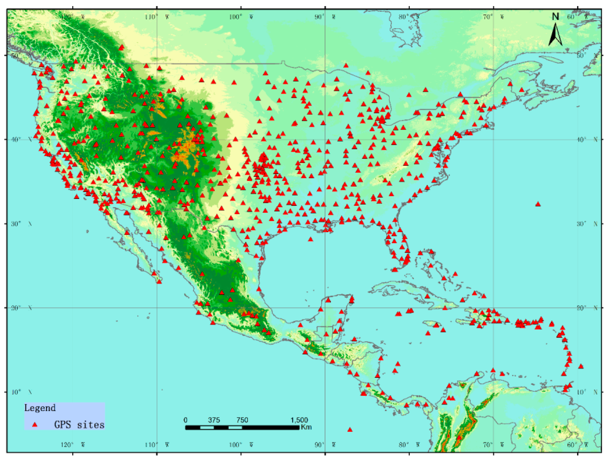
SuomiNet provides continuous TPW estimates from 828 sites distributed across the United States with accuracy better than 2 mm (~0.2 g/cm2) [8,38]. In this article, three years (2014–2017) of SuomiNet data are downloaded for the validation of the retrieved TPW. The geolocations of SuomiNet GPS stations are displayed in Figure 1.
2.2. The Joint Polar Satellite System (JPSS) Microwave Integrated Retrieval System (MIRS) Precipitation Product
The microwave integrated retrieval system (MIRS) was developed by the NOAA/National Environmental Satellite, Data, and Information Service (NESDIS) Center for Satellite Application and Research (STAR) and has been put into use in the NOAA/NESDIS Satellite and Product Operations Office (OSPO), which aims to upgrade the current operational microwave surface and precipitation products system (MSPPS) [39,40]. The operational MIRS can produce advanced near-real-time surface and precipitation products in all weather and over all surface conditions using brightness temperatures from the microwave instruments, such as the advanced technology microwave sounder (ATMS) onboard the S-NPP satellite. ATMS is a cross-track scanner with 22 channels in spectral bands from 23 GHz through 183 GHz [41]. The operational products of MIRS include vertical profiles of temperature and TPW, rainfall rate, cloud liquid water, snow cover, snow water equivalent, sea ice concentration, ice water path, and land surface temperature. The spatial resolution of the MIRS TPW product derived from ATMS is 15 km at Nadir. Suomi NPP orbits the Earth 14.1875 times each day in a Sun-synchronous, polar orbit that allows ATMS to observe nearly the entire global atmosphere twice daily.
2.3. Visible Infrared Imaging Radiometer Suite (VIIRS)
The Visible Infrared Imaging Radiometer Suite (VIIRS), aboard the joint NASA/NOAA Suomi National Polar-Orbiting Partnership (S-NPP) satellite, was developed based on the heritage of legacy instruments, including the advanced very high resolution radiometer (AVHRR) and MODIS. VIIRS has 22 spectral channels with wavelengths covering from 0.41 μm to 12.5 μm, which can be used for environmental monitoring and numerical weather forecasting. The results from the on-orbit verification in the postlaunch check-out, intensive calibration, and validation have shown that VIIRS is performing very well [42]. More than 20 environmental data records have been produced operationally from VIIRS data, including clouds, land surface temperature, sea surface temperature, aerosol optical thickness, ocean color, polar wind, vegetation fraction, aerosol, fire, snow and ice, vegetation index, etc. However, to our knowledge, VIIRS does not provide TPW product.
The VIIRS data utilized in this study include VIIRS sensor data records (SDR) and VIIRS cloud mask intermediate product (VCM). The VIIRS SDR contains the day–night channel, imagery channel, moderate resolution channel, and geolocation data. Two thermal-infrared channels of VIIRS, M15 (10.75 µm) and M16 (12.01 µm), are selected. The VIIRS VCM product is used to identify whether a pixel is clear or cloudy [43]. The pixels with a confident clear flag are identified as clear-sky pixels. In addition, geolocation and sensor view zenith angle data are also utilized.
2.4. Seebor Atmosphere Profile
This Seebor global profiles database (named SeeBor V5.0) consists of 15,704 profiles distributed all over the world [44]. The temperature profile of Seebor has 101 levels, and the corresponding atmospheric pressure varies from 1100 hPa to 0.005 hPa. The atmosphere profiles are collected from NOAA-88, a European Centre for Medium-Range Weather Forecasts(ECMWF) 60L training set, TIGR-3, ozonesondes from 8 NOAA Climate Monitoring and Diagnostics Laboratory (CMDL) sites, and radiosondes from 2004 in the Sahara Desert. All the profiles are checked with the following saturation criteria to eliminate the cloudy atmosphere profile, i.e., the relative humidity value for each profile at each level below the 250 hPa pressure level must be less than 90%.
3. Methods
3.1. Split-Window Covariance-Variance Ratio Method
Assuming that the atmosphere state is invariant within a certain area, and the variation of surface emissivity is minimal, the split-window covariance-variance ratio method (SWCVR) [22,23] retrieves the TPW using the channel transmission ratio of two split-window channels (approximately 11 μm and 12 μm). The transmittance ratio can be obtained from the TOA brightness temperature of the two split-window channels. The SWCVR is expressed as:
where represents total precipitable water, k represents pixel k, the subscripts i and j represent the channels 15 and 16 of the VIIRS, and represent transmittance and emissivity of VIIRS channel i respectively, represents TOA brightness temperature of VIIRS channel i for pixel k, represents mean TOA brightness temperature of VIIRS channel i over N neighboring pixels, and denotes the correlation coefficient of and over the N neighboring pixels, and is used to determine whether the previous assumption is valid in the derivation process of the transmittance ratio.
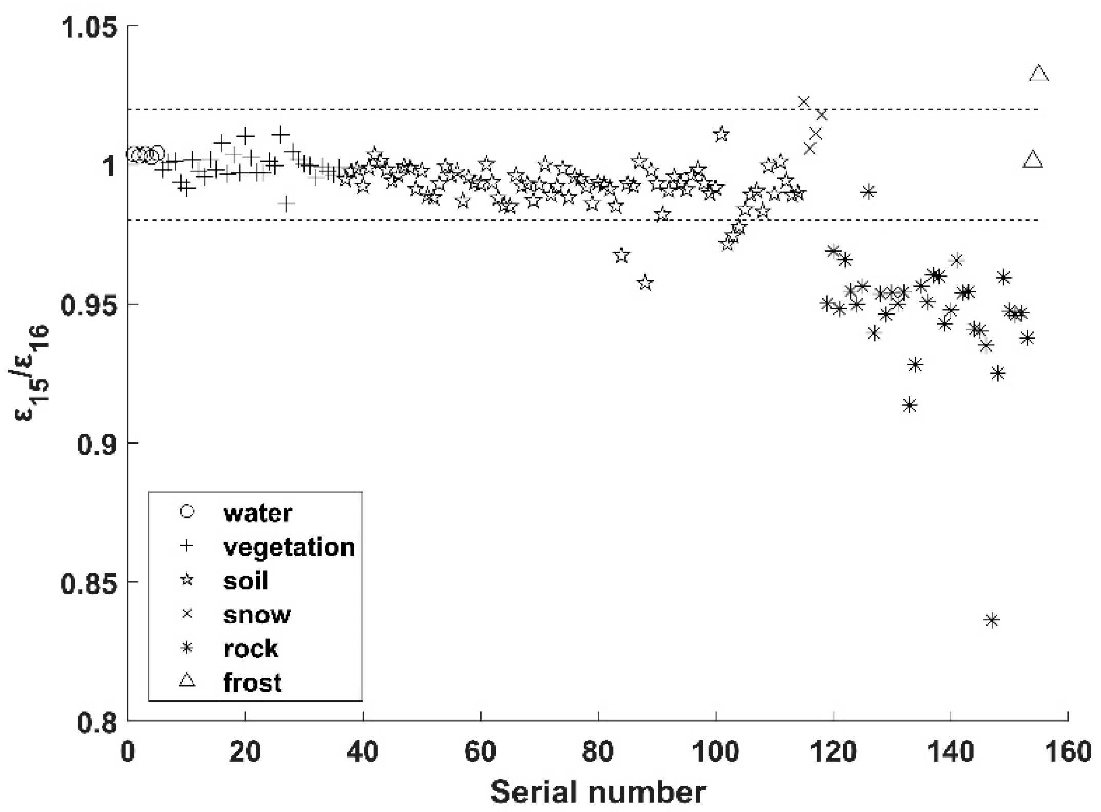
The transmission ratio can be retrieved using Equation (2) in the case that the emissivity ratio of two split-window channels is known. is calculated from the atmospheric top brightness temperature of the two split-window channels using Equation (3). The Advanced Spaceborne Thermal Emission and Reflection Radiometer(ASTER) emissivity library [45] and moderate resolution imaging spectroradiometer (MODIS) University of California, Santa Barbara(UCSB) emissivity library (https://icess.eri.ucsb.edu/modis/EMIS/html/em.html) is used to calculate the channel emissivity of VIIRS split-window channels. Figure 2 shows the variation of for different natural surface types including rocks, vegetation, soils, water, and snow. The emissivity ratios of channels 11 μm and 12 μm for most vegetation, water, snow, and soil are between 0.98 and 1.02. Considering that most pixels at a scale of 0.75 km are usually covered by soils, water, vegetation, snow, or their mixtures, the emissivity ratio can be approximated as unity in practice. Thus, the channel transmission ratio can be calculated as:
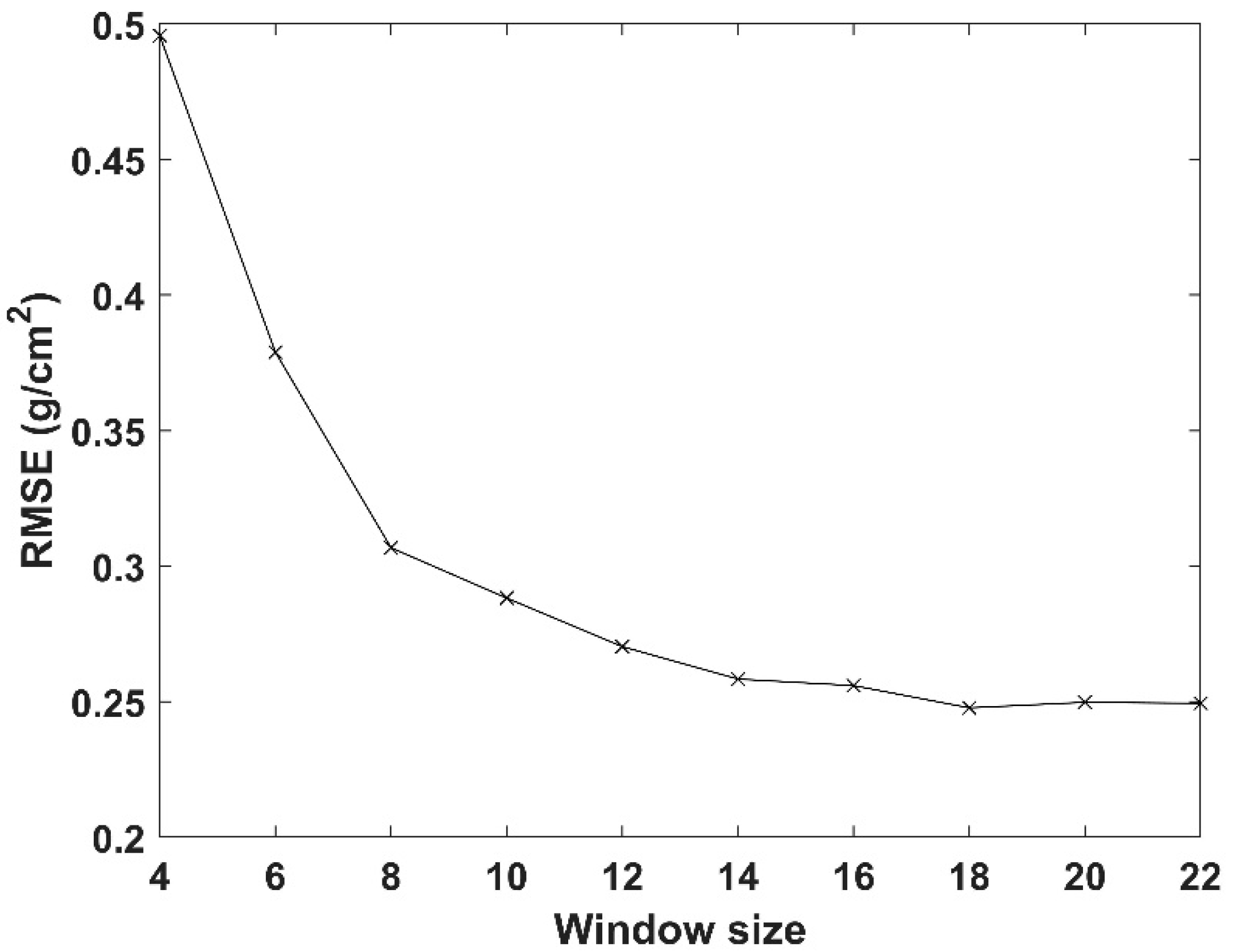
The number of neighboring pixels is a key parameter for the SWCVR method. The window size N (N × N neighboring pixels) should not be too large or too small, in case the atmospheric conditions may not be constant or cannot guarantee a high correlation between two channels’ TOA brightness temperatures [28]. A simple simulation experiment is conducted to investigate the effect of window size on the accuracy of the SWCVR method using the MODIS emissivity product MOD11B1. The emissivities of MODIS channels 31 and 32 are used as proxies of VIIRS channels M15 and M16, and the standard deviations of emissivities, approximately 0.01, are collected for different window sizes. The land surface temperature (LST) varies around the bottom layer temperature of different Seebor atmosphere profiles with a standard deviation of 2.5 K. The TOA brightness temperatures of VIIRS channels 15 and 16 are simulated using the moderate resolution atmospheric radiative transfer code (MODTRAN 5.0) for different window sizes. The TPW is retrieved using the SWCVR method from simulated VIIRS TOA brightness temperatures for different window sizes, and the root mean square error (RMSE) which are displayed in Figure 3. Obviously, the RMSE decreases as the window size increases, and the retrieval accuracy does not improve significantly with the increasing number of the neighboring pixels when the window is larger than 18. Therefore, the window size is set as 18 in this study.
The SWCVR algorithm is implemented in five steps:
- (1)
- Calculate the mean values of TOA brightness temperature and . Herein, the median values and are used instead of the mean values, as the median is a more robust estimator than the mean value.
- (2)
- Remove the cloudy pixels. The VIIRS cloud mask product is used to identify the cloudy pixels, and only confidently clear pixels are used to calculate .
- (3)
- Eliminate the invalid pixels. Since (at 12 μm) is smaller than (at 11 µm) and the ratio of emissivities is very close to unity for most conditions, should be smaller than unity. The absolute value of must be larger than the absolute value of and the values of and should have the same sign. Eliminating the invalid pixel can effectively avoid invalid inversion of transmittance ratios (i.e., a transmittance ratio lager than 1). For more details, please refer to Li et al. [23].
- (4)
- Estimate and reject if is less than 0.95.
- (5)
- Calculate the TPW for different view zenith angles. The relationship between TPW and the transmission ratio is established at several specific angles. When the view zenith angle is not equal to the specific angles, TPW is linearly interpolated from TPWs predicted by the model with an adjacent view zenith angle. View zenith angles exceeding 75° are not considered.
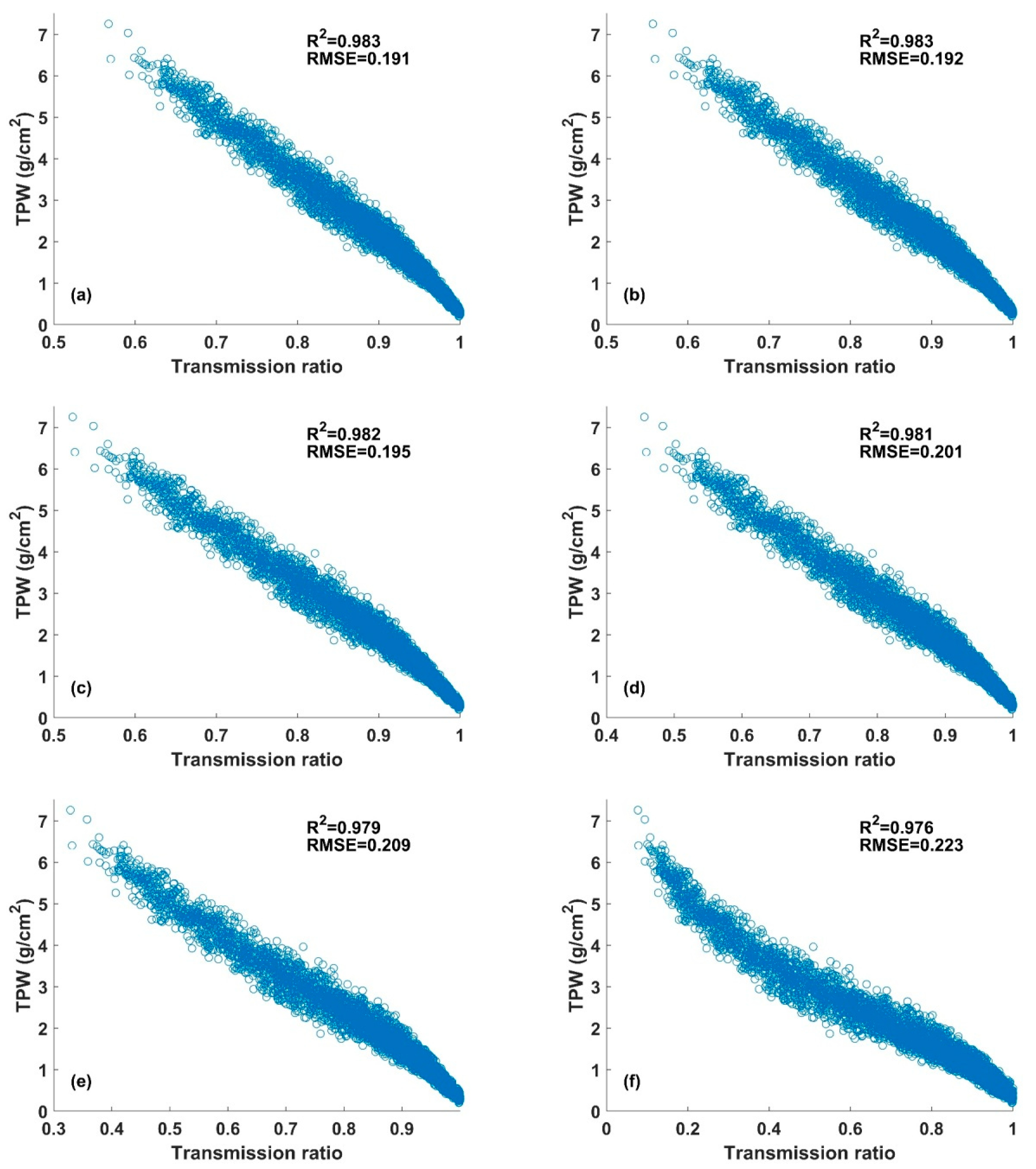
Figure 4 shows scatterplots of TPW versus the transmission ratio for VIIRS under different view angles (0°, 15°, 30°, 45°, 60°, 75°). The TPW and transmission ratio are simulated by MODTRAN 5 using Seebor atmosphere profiles and VIIRS filter response functions. The cubic polynomial is used to fit the relationship between matchup of the TPW of each Seebor atmosphere profile and corresponding VIIRS transmission ratio. The fitting results are provided in Table 1. The fitting accuracy decreases with the increasing view angle. The determination coefficient ranges from 0.976 to 0.983, and RMSE ranges from 0.191 to 0.223 g/cm2.
3.2. Bayesian Model Averaging
Bayesian model averaging (BMA) is a standard method for blending predictive distributions from different data sources when there are multiple models that may be statistically reasonable but it is unsure which one is the best [46,47,48]. BMA does not depend on a single “best” model, but fuses multiple models to obtain optimal results by considering the errors of different models, so the results of BMA are more stable than those of a single model. The BMA predictive probability density function (PDF) is a weighted average of PDFs centered on each of the models considered, where the weights of each model are equal to posterior probabilities of these models. The weights can reflect relative contributions of each model to the final output of the BMA model over the training period.
BMA can be used to obtain a more accurate and stable estimate of TPW by blending the TPW retrieved from the thermal infrared data and that retrieved from passive microwave data. For convenience, we denote the TPW value to be forecast from two data sources as y and the ground measurement at a certain time to be tpw. are forecast results from each model. According to the total probability formula, the forecast PDF is given by
where the is the forecast PDF based on alone and is the posterior probability of being correct given the training data. The posterior model probabilities add up to one, , such that they can be viewed as weights. The BMA predictive model is then
where is the posterior probability of forecast k. It is assumed the conditional PDF of y is normally distributed with mean and standard deviation , which can be written as:
In this case, the BMA predictive mean is the conditional expectation of y given the forecasts, namely
4. Results
4.1. Validating VIIRS TPW and MIRS-Derived TPW
Two indicators are selected to depict the accuracy of the derived TPW, the mean bias error (MBE) and root mean square error (RMSE). These indicators are defined as follows:
where N is the number of samples; is the true value of TPW, derived from atmosphere profile or measured by the ground-based GPS network; is the derived TPW.
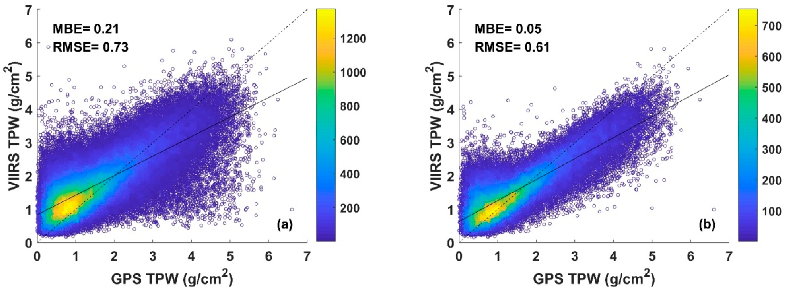
In this study, three years (2014–2017) of VIIRS data are used to derive the TPW using the refined SWCVR. The MIRS-derived TPW product synchronized in time and space with VIIRS is also extracted. The TPW measured by SuomiNet GPS receivers is used to validate the above two TPWs, Figure 5 and Figure 6 display the validation results. The MBE and RMSE of VIIRS TPW are 0.21 g/cm2 and 0.73 g/cm2, whereas MBE and RMSE of MIRS-derived TPW are 0.11 g/cm2 and 0.38 g/cm2. Clearly, the accuracy of MIRS-derived TPW is better than that of VIIRS TPW. Regarding the validation results for daytime and nighttime, no significant difference is found for MIRS-derived TPW. The MBE and RMSE are 0.12 g/cm2 and 0.39 g/cm2 for daytime, and 0.10 g/cm2 and 0.36 g/cm2 for nighttime. However, the accuracy of VIIRS TPW in daytime is better than that at nighttime. The MBE and RMSE are 0.05 g/cm2 and 0.61 g/cm2 for daytime, and 0.35 g/cm2 and 0.83 g/cm2 for nighttime. There may be two reasons for this result. First, the SWCVR may achieve good results when the surface emissivity varies little and the surface temperature varies greatly. However, the LST is more homogeneous in the nighttime than that in the daytime [51]. Second, cloud detection at night is worse than that in the daytime because there is no shortwave observation at night [52]. The VIIRS cloud mask cannot filter all cloudy pixels, and cannot entirely identify whether the pixels around the surface GPS station are confidently clear. This can partly explain the underestimation of VIIRS TPW under the high TPW condition in the nighttime. In addition, an obvious overestimation of VIIRS TPW can be found when TPW is low for both daytime and nighttime. The detailed reasons are discussed in a later section.
4.2. Blending TPWs Using BMA
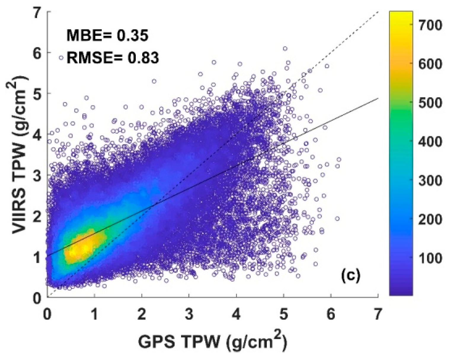
In this section, VIIRS TPW and clear-sky MIRS-derived TPW are integrated by BMA. The pixel spatial resolution difference between VIIRS TPW and MIRS-derived TPW is ignored during the process of integration. Two-thirds of the VIIRS TPW data and MIRS TPW data in the daytime are used for BMA model training, the remaining data (including one-third of the data in the daytime and all data in the nighttime) are used for validation. The blending results are displayed in Figure 7. The MBE and RMSE for BMA-derived TPW are 0.06 g/cm2 and 0.35 g/cm2, respectively, which is lower than that of MIRS-derived TPW (Figure 6a). Obviously, the accuracy of blended TPW is better than that of VIIRS TPW and MIRS-derived TPW on the whole, which demonstrates the good performance of BMA in integrating multi-source TPW data.
To further compare the three TPW data sets, we divided the validation results into four sub-regions according to the range of water vapor. The statistical results are provided in Table 2 and Table 3. The accuracy of MIRS-derived TPW and BMA-derived TPW are both better than the accuracy of VIIRS TPW. When the TPW is less than 3 g/cm2, the accuracy of BMA-derived TPW is better than that of MIRS-derived TPW. When the TPW is greater than 3 g/cm2, the accuracy of BMA-derived TPW is slightly worse than that of MIRS-derived TPW in the daytime and nighttime. This accuracy reducing may be caused by the undetected cloud pixels used in the SWCVR algorithm. With the upgrade of the VIIRS cloud detection algorithm, this problem may be alleviated to some extent. As a whole, blending VIIRS and MIRS-derived TPW using BMA improves the accuracy of TPW retrieval.
4.3. Production of VIIRS TPW
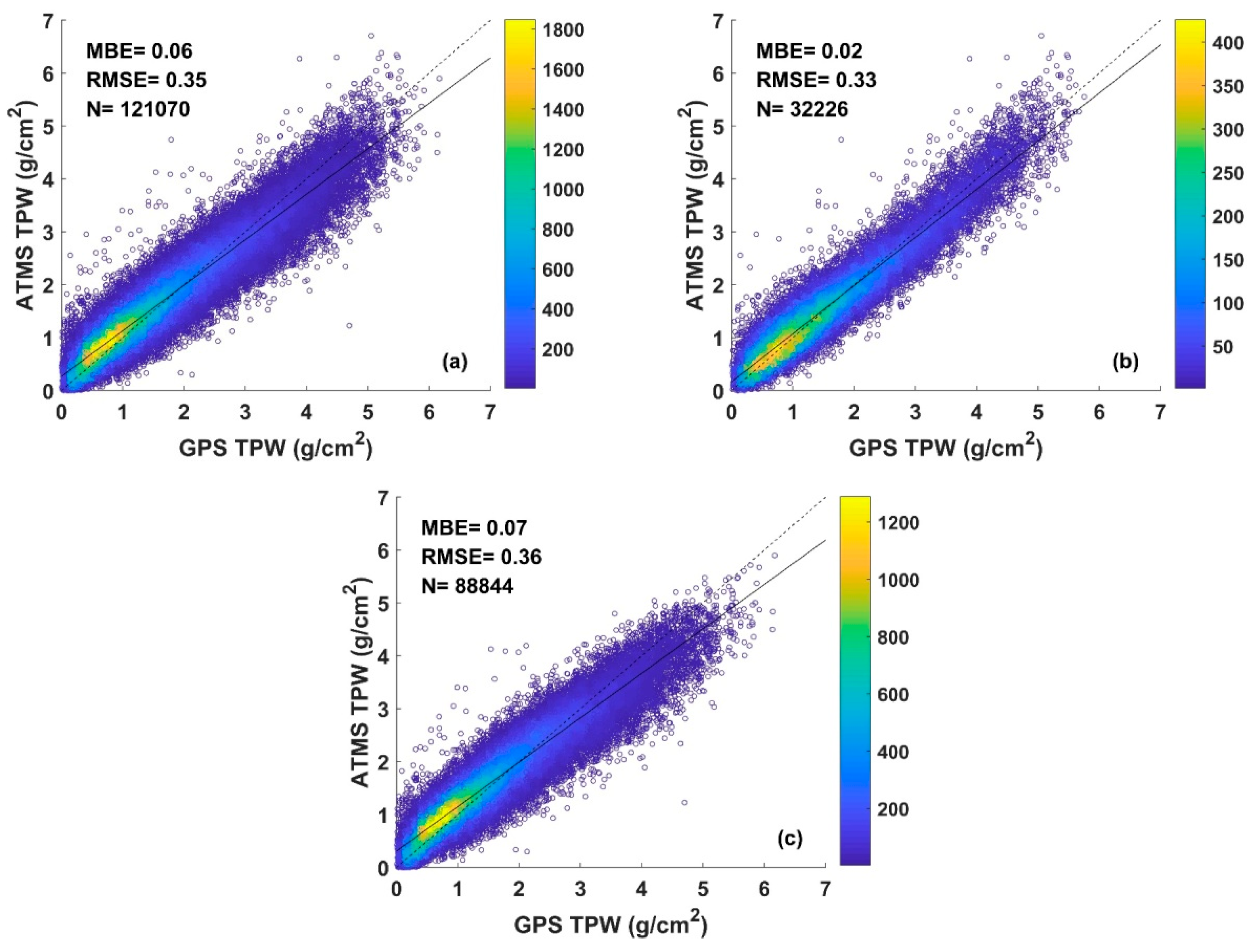
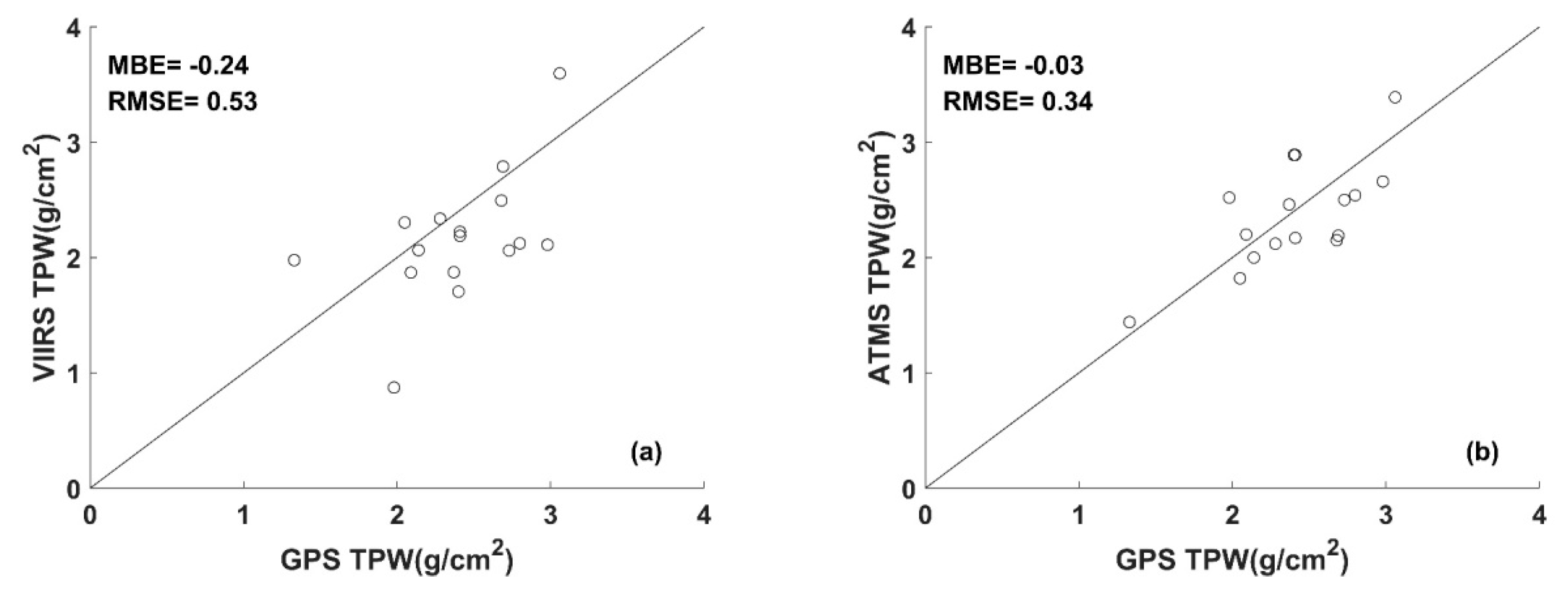
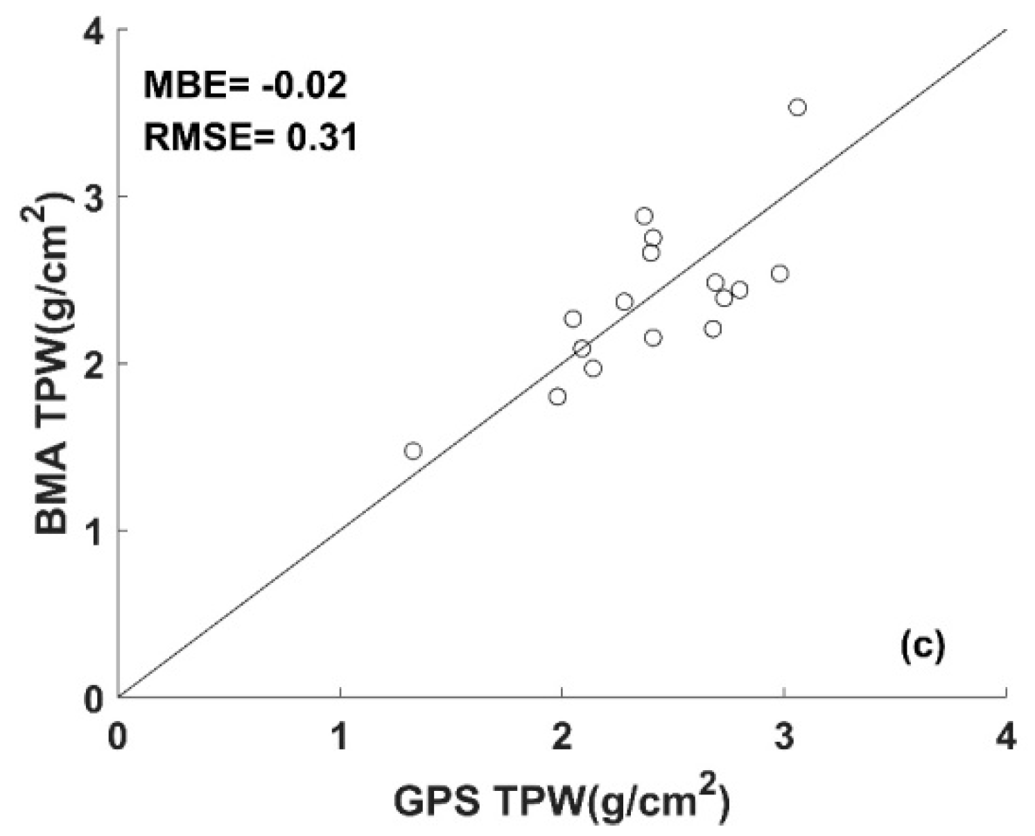
To examine the possibility of producing VIIRS TPW using the developed framework, we select a VIIRS granule image with relatively less cloud cover and the corresponding MIRS-derived TPW product beyond the acquisition time of validation data. The overpass time of the selected VIIRS granule image is at 20:18 (UTC), 25 September, 2018, and the MIRS-derived TPW product is acquired from 20:10 to 20:20 (UTC) on the same day. The VIIRS TPW is retrieved by the SWCVR method. The MIRS-derived TPW is interpolated to the VIIRS pixels using the nearest neighbor method. The resampled MIRS TPW is blended with VIIRS TPW using BMA. Figure 8 shows the produced BMA TPW, as well as VIIRS TPW and MIRS-derived TPW. The spatial pattern of VIIRS TPW is similar to that of MIRS-derived TPW, but the VIIRS TPW exhibits more details than the interpolated MIRS-derived TPW. The difference between TPW values in the VIIRS TPW and MIRS-derived TPW can be easily observed. The weight of MIRS-derived TPW is larger than that of VIIRS TPW because MIRS-derived TPW is more accurate than that of VIIRS TPW. Thus, the spatial pattern of BMA TPW is more similar to that of MIRS-derived TPW.
We also extract the SuomiNet TPW in the coverage of the VIIRS granule and validate three TPWs. The validation results are shown in Figure 9. The MBE and RMSE of BMA TPW are −0.024 and 0.314 g/cm2 respectively, which is superior to VIIRS TPW and comparable to MIRS-derived TPW whose MBE and RMSE are −0.238 and 0.535 g/cm2, and −0.029 and 0.337 g/cm2, respectively. This validation agrees with that presented in Section 4.2.
4.4. Validating BMA Integrated TPW Using Radiosonde Measurements
To verify the applicability of the BMA method in other areas, two years (2014–2015) of global climate observing system (GCOS) reference upper-air network (GRUAN) radiosonde data are collected. The GRUAN measurements provide appropriate data for studying atmospheric processes. Details about the GRUAN radiosonde measurements can be found at https://www.gruan.org. The TPW of radiosonde measurement is estimated by vertically integrating the specific humidity:
where is specific humidity, is acceleration of gravity, and is the atmospheric pressure.
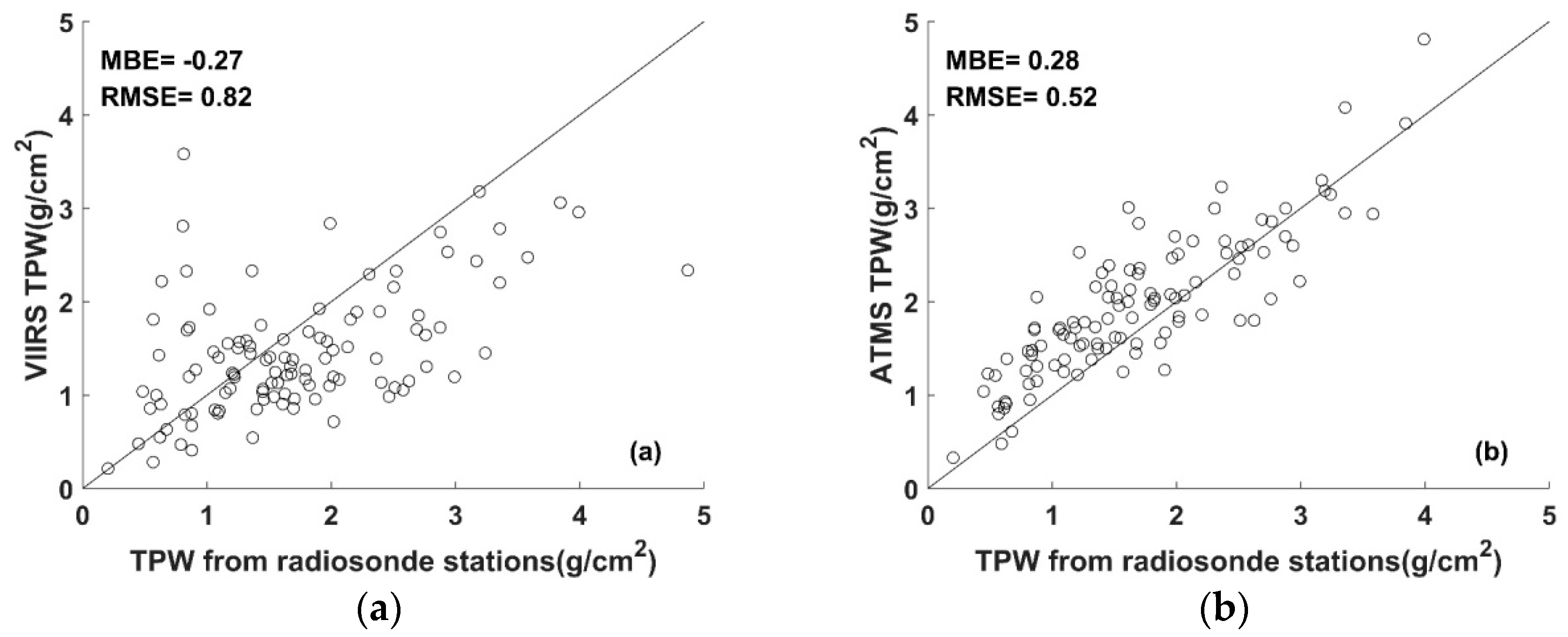
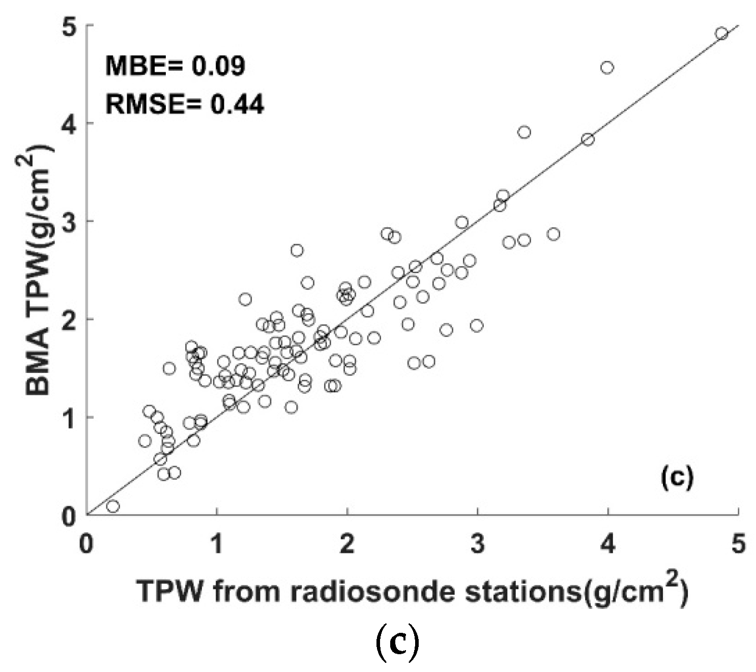
The VIIRS granule image is considered when the difference between the VIIRS overpass time and the balloon launch time is less than ten minutes. The VIIRS TPW is calculated using the SWCVR method, and then is blended with MIRS-derived TPW using the BMA method. According to Figure 10, the MBE and RMSE of BMA TPW are 0.09 g/cm2 and 0.44 g/cm2 when compared to the radiosonde measurements. The result is more accurate than both VIIRS TPW and MIRS-derived TPW, whose MBE and RMSE are −0.27 g/cm2 and 0.82 g/cm2, and 0.28 g/cm2 and 0.52 g/cm2, respectively. The results show that the BMA developed in North America can also be applied at a global scale.
5. Discussion
5.1. SWCVR
In Section 3, we explained that most of the emissivity ratios of two split-window channels for vegetation, water, snow, and soil are between 0.98 and 1.02, then that the transmission ratio of the split-window channel can be calculated using Equation (3). Since the transmittance in the channel at 12 μm is smaller than that in the channel at 11 μm, is smaller than unity. To avoid bad calculations of , the pixel filtering criteria proposed by Li et al. [23] is adopted, i.e., the absolute value of must be larger than the absolute value of , moreover, values of and should have the same sign. This criterion can ensure the rationality of the calculated transmission ratio and improve the accuracy of water vapor retrievals, which has been demonstrated in Li et al. [23]. However, it may cause underestimation of the transmission ratio under certain circumstances.
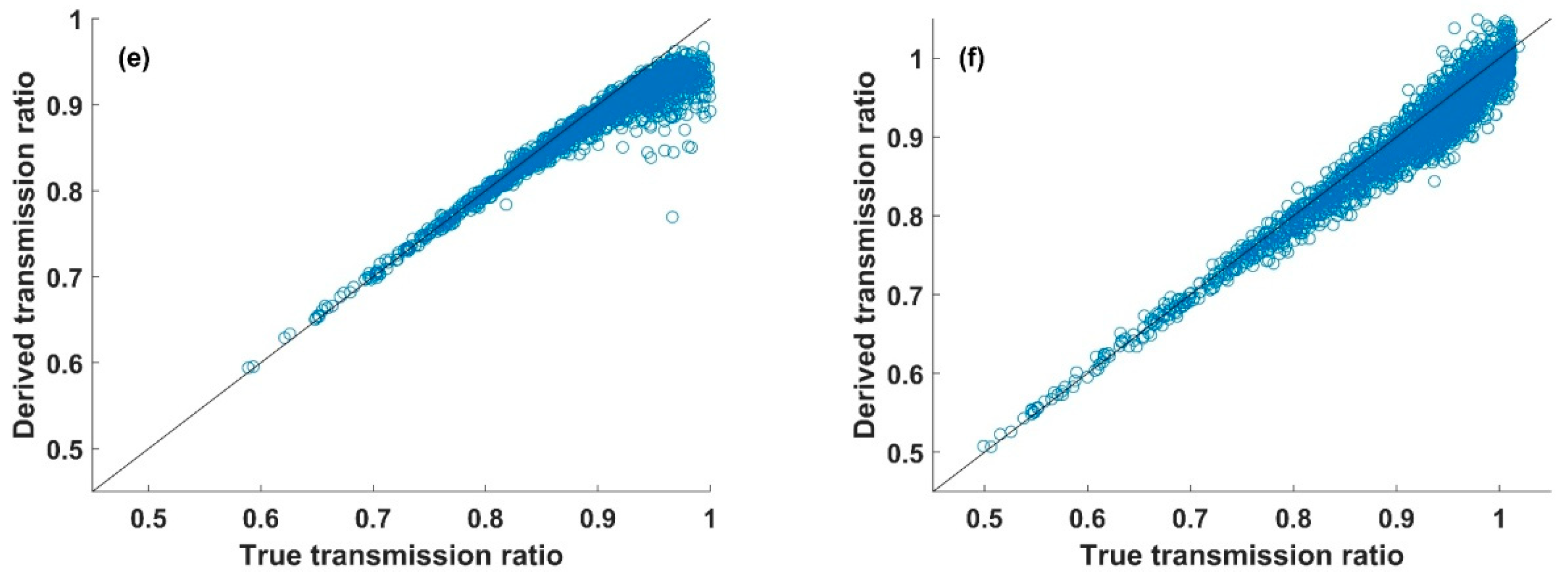
To exploit the effect of pixel filtering criteria in refined SWCVR, we conduct a simulation using MOD11B1 and Seebor atmosphere profiles. One year (2014) of MOD11B1 data covering North America is downloaded. An 18 × 18 window is used to extract the emissivities of channels 31 and 32. The spectral response functions of VIIRS channels 15 and 16 are similar to that of MODIS channel 31 and 32. The emissivities of VIIRS channels 15 and 16 are represented by MODIS channels 31 and 32 directly. The emissivity standard deviation for each window is also calculated. The surface temperature of these pixels is set as a Gaussian distribution, with the mean value equal to the bottom layer temperature of each Seebor atmosphere profile. The standard deviations are 2.5 K and 1 K for different conditions. The atmosphere transmission and TOA bright temperature of VIIRS are simulated using MODTRAN 5, and the atmosphere transmission ratio is calculated using Equation (2) with the simulated VIIRS TOA bright temperature. Detailed settings are provided in Table 4. Six sets of simulated data are separately used to calculate transmission ratios respectively. Then the calculated transmission ratio is compared to the true transmission ratio of each atmosphere profile. The comparison results are displayed in Figure 11. As shown in Figure 11, it is apparent that pixel filtering criteria can actually avoid unreasonable transmission ratios when using SWCVR. However, the criteria may cause underestimation of transmission ratios when the transmission ratio is greater than 0.85. Additionally, with the increase in the standard deviation of surface emissivity and the decrease in the standard deviation of surface temperature, the underestimation of transmission ratios becomes more significant under low TPW conditions (i.e., a transmission ratio lager than 0.85). Since the transmittance ratio is inversely proportional to the TPW, this can account for the overestimation of VIIRS TPW when the TPW is less than 1.5 g/cm2.
According to the above analysis, incorporating surface emissivity or normalized difference vegetation index (NDVI) data to select the relatively uniform part in the window size for TPW calculation in the SWCVR algorithm may improve the accuracy of the SWCVR method. This will be attempted in a future study.
5.2. The Limitations of this Study
A scale mismatch exists during the BMA integration of VIIRS TPW and MIRS-derived TPW. If both VIIRS and ATMS TPW are clear-sky pixels, it is reasonable to ignore the scale mismatch because the atmosphere is uniform. However, we cannot integrate VIIRS and ATMS TPW directly if the ATMS TPW pixel is partially cloudy, due to the fact that the 15 km ATMS pixel represents the overall water vapor state while VIIRS only represents the 750 m clear-sky condition. In order to deal with this condition, ATMS pixels need to be decomposed into clear sky and cloudy sky portions. Then the ATMS clear-sky TPW can be used to fuse with VIIRS TPW, and the cloudy sky TPW can be used to fill the gap of VIIRS TPW considering the scale effect. We will work on this in the future.
6. Conclusions
Atmospheric water content plays a pivotal role in atmospheric processes and the Earth’s climate. To our knowledge, VIIRS does not provide an operational TPW product. We developed a framework for estimating atmospheric TPW from Visible Infrared Imaging Radiometer Suite (VIIRS) data in this study. First, the refined SWCVR method was used to retrieve TPW from the VIIRS TOA brightness temperature of channels M15 and M16. Then a more accurate and stable TPW product was derived by blending the VIIRS TPW and MIRS-derived TPW using BMA.
The empirical relationships between TPW and channel transmission ratio were established at 0°, 15°, 30°, 45°, 60°, and 75° viewing angles using a huge amount of representative samples produced by extensive radiate transfer modeling. The established formulae accounted for more than 97.6% of the variation in the simulation database, the MBE was 0, and the RMSEs ranged from 0.19 g/cm2 to 0.22 g/cm2. Three years (2014–2017) of VIIRS data were used to retrieve TPW using the refined SWCVR. The retrieval results were validated using the ground measurements collected from SuomiNet sites over North America. The MBE and RMSE of VIIRS TPW were 0.21 g/cm2 and 0.73 g/cm2, respectively. The accuracy of VIIRS TPW in daytime was much better than at night time. The VIIRS TPW was blended with the MIRS-derived TPW product via BMA. The accuracy of MIRS-derived TPW was better than that of VIIRS TPW, with MBE and RMSE values of 0.11 g/cm2 and 0.38 g/cm2 when validated by the same data used for VIIRS TPW. The MBE and RMSE of BMA integrated TPW were 0.06 g/cm2 and 0.35 g/cm2, respectively, for which the accuracy difference in daytime and night time was removed. The global radiosonde measurements were also collected at the global scale to validate the BMA integrated VIIRS TPW. The MBE and RMSE of the BMA integrated TPW were 0.09 g/cm2 and 0.44 g/cm2 respectively compared to the radiosonde measurements, which was also more accurate than the VIIRS TPW. It was concluded that the developed framework can be used to derive accurate clear-sky TPW for VIIRS. This is the first time that we can obtain high accuracy TPW from VIIRS. This study will certainly benefit the study of atmospheric processes and climate change.
Author Contributions
J.C. conceived and designed the algorithm; J.C. and S.Z. performed the algorithm and analyzed the data; S.Z. wrote the paper. Both authors participated in the editing of the paper.
Funding
This work was partly supported by the National Natural Science Foundation of China via grant 41771365, the National Key Research and Development Program of China via grant 2016YFA0600101, and the Special Fund for Young Talents of the State Key Laboratory of Remote Sensing Sciences via grant 17ZY-02.
Acknowledgments
The ground data used in this study were collected from SUOMINET (https://www.suominet.ucar.edu). The global clear-sky Seebor atmosphere profile product was downloaded from CIMSS (https://cimss.ssec.wisc.edu/training_data/). The VIIRS SDR, cloud mask product, and microwave integrated retrieval system (MIRS) precipitation product were downloaded from NOAA (https://www.class.ngdc.noaa.gov/saa/products/welcome).
Conflicts of Interest
The authors declare no conflicts of interest.
References
- Lindstrot, R.; Stengel, M.; Schröder, M.; Fischer, J.; Preusker, R.; Schneider, N.; Steenbergen, T. A global climatology of total columnar water vapour from ssm/i and meris. Earth Syst. Sci. Data 2014, 6, 221–233. [Google Scholar] [CrossRef]
- Bosilovich, M.G.; Schubert, S.D. Water vapor tracers as diagnostics of the regional hydrologic cycle. J. Hydrometeorol. 2002, 3, 149–165. [Google Scholar] [CrossRef]
- Sellers, P.; Dickinson, R.; Randall, D.; Betts, A.; Hall, F.; Berry, J.; Collatz, G.; Denning, A.; Mooney, H.; Nobre, C. Modeling the exchanges of energy, water, and carbon between continents and the atmosphere. Science 1997, 275, 502–509. [Google Scholar] [CrossRef]
- Soden, B.J.; Wetherald, R.T.; Stenchikov, G.L.; Robock, A. Global cooling after the eruption of mount pinatubo: A test of climate feedback by water vapor. Science 2002, 296, 727–730. [Google Scholar] [CrossRef] [PubMed]
- Elliott, W.P.; Gaffen, D.J. On the utility of radiosonde humidity archives for climate studies. Bull. Am. Meteorol. Soc. 1991, 72, 1507–1520. [Google Scholar] [CrossRef]
- Han, Y.; Snider, J.; Westwater, E.; Melfi, S.; Ferrare, R. Observations of water vapor by ground-based microwave radiometers and raman lidar. J. Geophys. Res. Atmos. 1994, 99, 18695–18702. [Google Scholar] [CrossRef]
- Whiteman, D.; Evans, K.; Demoz, B.; Starr, D.O.C.; Eloranta, E.; Tobin, D.; Feltz, W.; Jedlovec, G.; Gutman, S.; Schwemmer, G. Raman lidar measurements of water vapor and cirrus clouds during the passage of hurricane bonnie. J. Geophys. Res. Atmos. 2001, 106, 5211–5225. [Google Scholar] [CrossRef]
- Ware, R.H.; Fulker, D.W.; Stein, S.A.; Anderson, D.N.; Avery, S.K.; Clark, R.D.; Droegemeier, K.K.; Kuettner, J.P.; Minster, J.B.; Sorooshian, S. Suominet: A real-time national gps network for atmospheric research and education. Bull. Am. Meteorol. Soc. 2000, 81, 677–694. [Google Scholar] [CrossRef]
- Gao, B.C.; Kaufman, Y.J. Water vapor retrievals using moderate resolution imaging spectroradiometer (modis) near-infrared channels. J. Geophys. Res. Atmos. 2003, 108, D13. [Google Scholar] [CrossRef]
- Gao, B.; Goetz, A.; Westwater, E.R.; Conel, J.; Green, R. Possible near-ir channels for remote sensing precipitable water vapor from geostationary satellite platforms. J. Appl. Meteorol. 1993, 32, 1791–1801. [Google Scholar] [CrossRef]
- Kleidman, R.G.; Kaufman, Y.J.; Gao, B.C.; Remer, L.A.; Brackett, V.G.; Ferrare, R.A.; Browell, E.V.; Ismail, S. Remote sensing of total precipitable water vapor in the near-ir over ocean glint. Geophys. Res. Lett. 2000, 27, 2657–2660. [Google Scholar] [CrossRef]
- Wang, J.; Wilheit, T.; Chang, L. Retrieval of total precipitable water using radiometric measurements near 92 and 183 ghz. J. Appl. Meteorol. 1989, 28, 146–154. [Google Scholar] [CrossRef]
- Alishouse, J.C.; Snyder, S.A.; Vongsathorn, J.; Ferraro, R.R. Determination of oceanic total precipitable water from the ssm/i. IEEE Trans. Geosci. Remote Sens. 1990, 28, 811–816. [Google Scholar] [CrossRef]
- Du, J.; Kimball, J.S.; Jones, L.A. Satellite microwave retrieval of total precipitable water vapor and surface air temperature over land from amsr2. IEEE Trans. Geosci. Remote Sens. 2015, 53, 2520–2531. [Google Scholar] [CrossRef]
- Aires, F.; Bernardo, F.; Prigent, C. Atmospheric water-vapour profiling from passive microwave sounders over ocean and land. Part I: Methodology for the megha-tropiques mission. Q. J. R. Meteorol. Soc. 2013, 139, 852–864. [Google Scholar] [CrossRef]
- Grody, N.; Zhao, J.; Ferraro, R.; Weng, F.; Boers, R. Determination of precipitable water and cloud liquid water over oceans from the noaa 15 advanced microwave sounding unit. J. Geophys. Res. Atmos. 2001, 106, 2943–2953. [Google Scholar] [CrossRef]
- Kleespies, T.J.; McMillin, L.M. Retrieval of precipitable water from observations in the split window over varying surface temperatures. J. Appl. Meteorol. 1990, 29, 851–862. [Google Scholar] [CrossRef]
- Chesters, D.; Robinson, W.D.; Uccellini, L.W. Optimized retrievals of precipitable water from the vas “split window”. J. Clim. Appl. Meteorol. 1987, 26, 1059–1066. [Google Scholar] [CrossRef]
- Andersen, H.S. Estimation of precipitable water vapour from noaa-avhrr data during the hapex sahel experiment. Int. J. Remote Sens. 1996, 17, 2783–2801. [Google Scholar] [CrossRef]
- Seemann, S.W.; Li, J.; Menzel, W.P.; Gumley, L.E. Operational retrieval of atmospheric temperature, moisture, and ozone from modis infrared radiances. J. Appl. Meteorol. 2003, 42, 1072–1091. [Google Scholar] [CrossRef]
- Jedlovec, G.J. Precipitable water estimation from high-resolution split window radiance measurements. J. Appl. Meteorol. 1990, 29, 863–877. [Google Scholar] [CrossRef]
- Sobrino, J.A.; Li, Z.-L.; Stoll, M.P.; Becker, F. Improvements in the split-window technique for land surface temperature determination. IEEE Trans. Geosci. Remote Sens. 1994, 32, 243–253. [Google Scholar] [CrossRef]
- Li, Z.-L.; Jia, L.; Su, Z.; Wan, Z.; Zhang, R. A new approach for retrieving precipitable water from atsr2 split-window channel data over land area. Int. J. Remote Sens. 2003, 24, 5095–5117. [Google Scholar] [CrossRef]
- Barducci, A.; Guzzi, D.; Marcoionni, P.; Pippi, I. Algorithm for the retrieval of columnar water vapor from hyperspectral remotely sensed data. Appl. Opt. 2004, 43, 5552–5563. [Google Scholar] [CrossRef]
- Hagan, D.; Webster, C.; Farmer, C.; May, R.; Herman, R.; Weinstock, E.; Christensen, L.; Lait, L.; Newman, P.A. Validating airs upper atmosphere water vapor retrievals using aircraft and balloon in situ measurements. Geophys. Res. Lett. 2004, 31, 21. [Google Scholar] [CrossRef]
- Ji, D.; Shi, J.; Xiong, C.; Wang, T.; Zhang, Y. A total precipitable water retrieval method over land using the combination of passive microwave and optical remote sensing. Remote Sens. Environ. 2017, 191, 313–327. [Google Scholar] [CrossRef]
- Wang, M.; He, G.; Zhang, Z.; Wang, G.; Long, T. NDVI-based split-window algorithm for precipitable water vapour retrieval from Landsat-8 TIRS data over land area. Remote Sens. Lett. 2015, 6, 904–913. [Google Scholar] [CrossRef]
- Ren, H.; Du, C.; Liu, R.; Qin, Q.; Yan, G.; Li, Z.L.; Meng, J. Atmospheric water vapor retrieval from landsat 8 thermal infrared images. J. Geophys. Res. Atmos. 2015, 120, 1723–1738. [Google Scholar] [CrossRef]
- Zhou, S.; Cheng, J. Estimation of high spatial-resolution clear-sky land surface-upwelling longwave radiation from viirs/s-npp data. Remote Sens. 2018, 10, 253. [Google Scholar] [CrossRef]
- Cheng, J.; Liang, S.; Wang, W.; Guo, Y. An efficient hybrid method for estimating clear-sky surface downward longwave radiation from modis data. J. Geophys. Res. Atmos. 2017, 122, 2616–2630. [Google Scholar] [CrossRef]
- Cheng, J.; Liang, S. Global estimates for high spatial resolution clear-sky land surface upwelling longwave radiation from modis data. IEEE Trans. Geosci. Remote Sens. 2016, 54, 4115–4129. [Google Scholar] [CrossRef]
- Cheng, J.; Yang, F.; Guo, Y. A comparative study of bulk parameterization schemes for estimating cloudy-sky surface downward longwave radiation. Remote Sens. 2019, 11, 528. [Google Scholar] [CrossRef]
- Guo, Y.; Cheng, J.; Liang, S. Comprehensive assessment of parameterization methods for estimating clear-sky surface downward longwave radiation. Theor. Appl. Climatol. 2019, 135, 1045–1058. [Google Scholar] [CrossRef]
- Guo, Y.; Cheng, J. Feasibility of estimating cloudy-sky surface longwave net radiation using satellite-derived surface shortwave net radiation. Remote Sens. 2018, 10, 596. [Google Scholar] [CrossRef]
- Ware, R.; Braun, J.; Ha, S.; Hunt, D.; Kuo, Y.; Rocken, C.; Sleziak, M.; Van Hove, T.; Weber, J.; Anthes, R. Real-time water vapor sensing with suominet—Today and tomorrow. In Proceedings of the International GPS Meteorology Workshop, Tsukuba, Japan, 14–17 January 2003. [Google Scholar]
- Mears, C.A.; Wang, J.; Smith, D.; Wentz, F.J. Intercomparison of total precipitable water measurements made by satellite-borne microwave radiometers and ground-based gps instruments. J. Geophys. Res. Atmos. 2015, 120, 2492–2504. [Google Scholar] [CrossRef]
- Rocken, C.; Hove, T.V.; Johnson, J.; Solheim, F.; Ware, R.; Bevis, M.; Chiswell, S.; Businger, S. Gps/storm—gps sensing of atmospheric water vapor for meteorology. J. Atmos. Ocean. Technol. 1995, 12, 468–478. [Google Scholar] [CrossRef]
- Rocken, C.; Ware, R.; Van Hove, T.; Solheim, F.; Alber, C.; Johnson, J.; Bevis, M.; Businger, S. Sensing atmospheric water vapor with the global positioning system. Geophys. Res. Lett. 1993, 20, 2631–2634. [Google Scholar] [CrossRef]
- Boukabara, S.; Weng, F.; Ferraro, R.; Zhao, L.; Liu, Q.; Yan, B.; Li, A.; Chen, W.; Sun, N.; Meng, H. In Introducing noaa’s microwave integrated retrieval system (mirs). In Proceedings of the 15th International TOVS Study Conference (ITSC-15), Maratea, Italy, 4–10 October 2006. [Google Scholar]
- Boukabara, S.-A.; Garrett, K.; Chen, W.; Iturbide-Sanchez, F.; Grassotti, C.; Kongoli, C.; Chen, R.; Liu, Q.; Yan, B.; Weng, F. Mirs: An all-weather 1dvar satellite data assimilation and retrieval system. IEEE Trans. Geosci. Remote Sens. 2011, 49, 3249–3272. [Google Scholar] [CrossRef]
- Muth, C.; Lee, P.S.; Shiue, J.C.; Webb, W.A. Advanced technology microwave sounder on npoess and npp. In Proceedings of the Geoscience and Remote Sensing Symposium (IGARSS’04), Anchorage, AK, USA, 20–24 September 2004; pp. 2454–2458. [Google Scholar]
- Cao, C.; Xiong, J.; Blonski, S.; Liu, Q.; Uprety, S.; Shao, X.; Bai, Y.; Weng, F. Suomi npp viirs sensor data record verification, validation, and long-term performance monitoring. J. Geophys. Res. Atmos. 2013, 118, 11664–11678. [Google Scholar] [CrossRef]
- Kopp, T.J.; Thomas, W.; Heidinger, A.K.; Botambekov, D.; Frey, R.A.; Hutchison, K.D.; Iisager, B.D.; Brueske, K.; Reed, B. The viirs cloud mask: Progress in the first year of s-npp toward a common cloud detection scheme. J. Geophys. Res. Atmos. 2014, 119, 2441–2456. [Google Scholar] [CrossRef]
- Borbas, E.; Seemann, S.W.; Huang, H.-L.; Li, J.; Menzel, W.P. Global profile training database for satellite regression retrievals with estimates of skin temperature and emissivity. In Proceedings of the 14th International ATOVS Study Conference, Beijing, China, 25–31 May 2005; pp. 763–770. [Google Scholar]
- Baldridge, A.; Hook, S.; Grove, C.; Rivera, G. The aster spectral library version 2.0. Remote Sens. Environ. 2009, 113, 711–715. [Google Scholar] [CrossRef]
- Hoeting, J.A.; Madigan, D.; Raftery, A.E.; Volinsky, C.T. Bayesian model averaging: A tutorial. Stat. Sci. 1999, 14, 382–401. [Google Scholar]
- Raftery, A.E.; Gneiting, T.; Balabdaoui, F.; Polakowski, M. Using bayesian model averaging to calibrate forecast ensembles. Mon. Weather Rev. 2005, 133, 1155–1174. [Google Scholar] [CrossRef]
- Claeskens, G.; Hjort, N.L. Model Selection and Model Averaging; Cambridge University Press: Cambridge, UK, 2008. [Google Scholar]
- Fisher, R.A. On the mathematical foundations of theoretical statistics. Philos. Trans. R. Soc. Lond. A 1922, 222, 309–368. [Google Scholar] [CrossRef]
- Moon, T.K. The expectation-maximization algorithm. IEEE Signal Process. Mag. 1996, 13, 47–60. [Google Scholar] [CrossRef]
- Wang, W.; Liang, S.; Meyers, T. Validating modis land surface temperature products using long-term nighttime ground measurements. Remote Sens. Environ. 2008, 112, 623–635. [Google Scholar] [CrossRef]
- Frey, R.; Heidinger, A.; Hutchison, K.; Botambekov, D.; Dutcher, S. Viirs cloud mask validation exercises. Polar 2011, 82, 84–89. [Google Scholar]
Figure 1.
Location of SuomiNet GPS stations in North American.

Figure 2.
Emissivity ratios of VIIRS channels 15 and 16 calculated from ASTER emissivity library and the MODIS UCSB emissivity library (sample serial number versus emissivity ratio).
Figure 2.
Emissivity ratios of VIIRS channels 15 and 16 calculated from ASTER emissivity library and the MODIS UCSB emissivity library (sample serial number versus emissivity ratio).

Figure 3.
Influence of window size on the accuracy of split-window covariance-variance ratio method (SWCVR) using simulation data.
Figure 3.
Influence of window size on the accuracy of split-window covariance-variance ratio method (SWCVR) using simulation data.

Figure 4.
The relationship between the transmission ratio of VIIRS and total precipitable water (TPW) for different view zenith angles. (a) 0°, (b) 15°, (c) 30°, (d) 45°, (e) 60°, and (f) 75°.
Figure 4.
The relationship between the transmission ratio of VIIRS and total precipitable water (TPW) for different view zenith angles. (a) 0°, (b) 15°, (c) 30°, (d) 45°, (e) 60°, and (f) 75°.

Figure 5.
Comparison of VIIRS TPW retrieved by the refined SWCVR with that measured by ground-based GPS. (a) All; (b) daytime; (c) nighttime.
Figure 5.
Comparison of VIIRS TPW retrieved by the refined SWCVR with that measured by ground-based GPS. (a) All; (b) daytime; (c) nighttime.


Figure 6.
Comparison of microwave integrated retrieval system (MIRS)-derived TPW with that measured by ground-based GPS. (a) All; (b) daytime; (c) nighttime.
Figure 6.
Comparison of microwave integrated retrieval system (MIRS)-derived TPW with that measured by ground-based GPS. (a) All; (b) daytime; (c) nighttime.

Figure 7.
Validation results of blended TPW using Bayesian model averaging (BMA). (a) All; (b) daytime; (c) nighttime.
Figure 7.
Validation results of blended TPW using Bayesian model averaging (BMA). (a) All; (b) daytime; (c) nighttime.

Figure 8.
Spatial pattern of VIIRS TPW, MIRS-derived TPW, and BMA TPW.

Figure 9.
The scatterplots of derived TPW with respect to GPS TPW. (a) VIIRS TPW, (b) MIRS-derived TPW, (c) BMA TPW.
Figure 9.
The scatterplots of derived TPW with respect to GPS TPW. (a) VIIRS TPW, (b) MIRS-derived TPW, (c) BMA TPW.


Figure 10.
The scatterplots of derived TPW with respect to TPW calculated from radiosonde stations. (a) VIIRS TPW, (b) MIRS-derived TPW, (c) BMA integrated TPW.
Figure 10.
The scatterplots of derived TPW with respect to TPW calculated from radiosonde stations. (a) VIIRS TPW, (b) MIRS-derived TPW, (c) BMA integrated TPW.


Figure 11.
Scatterplots of derived channel transmission ratios versus true transmission ratios under different surface conditions. (a) Case 1; (b) case 2; (c) case 3; (d) case 4; (e) case 5; (f) case 6.
Figure 11.
Scatterplots of derived channel transmission ratios versus true transmission ratios under different surface conditions. (a) Case 1; (b) case 2; (c) case 3; (d) case 4; (e) case 5; (f) case 6.


Table 1.
The fitted relationship between TPW and VIIRS transmittance ratios for different view angles.
Table 1.
The fitted relationship between TPW and VIIRS transmittance ratios for different view angles.
| View Angle | Expression for TPW | R2 | RMSE (g/cm2) |
|---|---|---|---|
| 0° | w = −43.383x3 + 96.438x2 − 85.266x + 32.297 | 0.983 | 0.191 |
| 15° | w = −42.366x3 + 93.886x2 − 82.8x + 31.365 | 0.983 | 0.192 |
| 30° | w = −39.201x3 + 85.956x2 − 75.185x + 28.512 | 0.982 | 0.195 |
| 45° | w = −33.231x3 + 71.142x2 − 61.309x + 23.475 | 0.981 | 0.201 |
| 60° | w = −23.846x3 + 48.527x2 − 40.888x + 16.288 | 0.979 | 0.209 |
| 75° | w = −12.322x3 + 22.69x2 − 18.262x + 7.9912 | 0.976 | 0.223 |
Table 2.
Validation results of three TPW data sets for the daytime.
| TPW Range | Data | MBE (g/cm2) | RMSE (g/cm2) |
|---|---|---|---|
| Total | BMA | 0.023 | 0.332 |
| VIIRS | 0.049 | 0.605 | |
| MIRS | 0.117 | 0.391 | |
| <1.5 g/cm2 | BMA | 0.099 | 0.301 |
| VIIRS | 0.320 | 0.588 | |
| MIRS | 0.212 | 0.371 | |
| [1.5 g/cm2, 3 g/cm2] | BMA | –0.062 | 0.328 |
| VIIRS | –0.177 | 0.445 | |
| MIRS | 0.024 | 0.372 | |
| >3 g/cm2 | BMA | –0.142 | 0.457 |
| VIIRS | –0.702 | 0.921 | |
| MIRS | –0.114 | 0.511 |
Table 3.
Validation results of three TPW data sets for the night time.
| TPW Range | Data | MBE (g/cm2) | RMSE (g/cm2) |
|---|---|---|---|
| Total | BMA | 0.074 | 0.356 |
| VIIRS | 0.354 | 0.826 | |
| MIRS | 0.098 | 0.363 | |
| <1.5 g/cm2 | BMA | 0.131 | 0.309 |
| VIIRS | 0.250 | 0.808 | |
| MIRS | 0.144 | 0.327 | |
| [1.5 g/cm2, 3 g/cm2] | BMA | 0.013 | 0.356 |
| VIIRS | 0.142 | 0.628 | |
| MIRS | 0.016 | 0.365 | |
| >3 g/cm2 | BMA | –0.355 | 0.568 |
| VIIRS | –0.710 | 1.320 | |
| MIRS | –0.351 | 0.530 |
Table 4.
Transmittance ratio accuracy for different surface conditions and pixel selection criteria.
Table 4.
Transmittance ratio accuracy for different surface conditions and pixel selection criteria.
| Cases | LST Standard Deviation (K) | Emissivity Standard Deviation | Pixel Selection Criteria | MBE | RMSE |
|---|---|---|---|---|---|
| 1 | 2.5 | 0.02 | –0.06 | 0.07 | |
| 2 | 2.5 | 0.02 | -- | 0.01 | 0.02 |
| 3 | 1 | 0.02 | Same as case 1 | –0.11 | 0.13 |
| 4 | 1 | 0.02 | -- | 0.07 | 0.12 |
| 5 | 2.5 | 0.01 | Same as case 1 | –0.02 | 0.03 |
| 6 | 2.5 | 0.01 | -- | –0.01 | 0.02 |
© 2019 by the authors. Licensee MDPI, Basel, Switzerland. This article is an open access article distributed under the terms and conditions of the Creative Commons Attribution (CC BY) license (http://creativecommons.org/licenses/by/4.0/).
Share and Cite
MDPI and ACS Style
Zhou, S.; Cheng, J. A Framework for Estimating Clear-Sky Atmospheric Total Precipitable Water (TPW) from VIIRS/S-NPP. Remote Sens. 2019, 11, 916. https://doi.org/10.3390/rs11080916
AMA Style
Zhou S, Cheng J. A Framework for Estimating Clear-Sky Atmospheric Total Precipitable Water (TPW) from VIIRS/S-NPP. Remote Sensing. 2019; 11(8):916. https://doi.org/10.3390/rs11080916
Chicago/Turabian StyleZhou, Shugui, and Jie Cheng. 2019. "A Framework for Estimating Clear-Sky Atmospheric Total Precipitable Water (TPW) from VIIRS/S-NPP" Remote Sensing 11, no. 8: 916. https://doi.org/10.3390/rs11080916
Note that from the first issue of 2016, this journal uses article numbers instead of page numbers. See further details here.