Mapping Forest Type and Tree Species on a Regional Scale Using Multi-Temporal Sentinel-2 Data


Institute of Geodesy and Cartography, Remote Sensing Centre, Modzelewskiego 27, 02-679 Warsaw, Poland
*
Author to whom correspondence should be addressed.
Remote Sens. 2019, 11(8), 929; https://doi.org/10.3390/rs11080929
Submission received: 3 April 2019
/
Revised: 9 April 2019
/
Accepted: 15 April 2019
/
Published: 17 April 2019
(This article belongs to the Special Issue Remote sensing based Forest Inventories from Landscape to Global Scale)
Abstract
:There are a limited number of studies addressing the forest status, its extent, location, type and composition over a larger area at the regional or national levels. The dense time series and a wide swath of Sentinel-2 data are a good basis for forest mapping and tree species identification over a large area. This study presents the results of the classification of the forest/non-forest cover, forest type (broadleaf and coniferous) and the identification of eight tree species (beech, oak, alder, birch, spruce, pine, fir, and larch) using the multi-temporal Sentinel-2 data in combination with topographic information. The study was conducted over the large mountain area located in southern Poland. The Random Forest classifier was used to first derive a forest/non-forest map. Second, the forest was classified into broadleaf and coniferous. Finally, the tree species classification was carried out following two approaches: (i) Non-stratified, where all species were classified together within the forest mask and (ii) stratified, where the broadleaf and coniferous tree species were classified separately within the forest type masks. The overall accuracy for the forest/non-forest cover reached 98.3% and declined slightly to 94.8% for the classification of the forest type. The use of the topographic information did not increase the accuracy of either result. The role of the topographic variables increased significantly in the process of tree species delineation. By combining the topographic information (in particular, digital elevation model) with the multi-temporal Sentinel-2 data, the classification of eight tree species improved from 75.6% to 81.7% (approach 1). A further increase in accuracy to 89.5% for broadleaf and 82% for coniferous species was observed following the stratified approach number 2. The highest overall accuracy (above 85%) was obtained for beech, oak, birch, alder, and larch. The study confirmed the potential of the multi-temporal Sentinel-2 data for accurate delineation of the forest cover, forest type, and tree species at the regional scale.
1. Introduction
Accurate and up-to-date information on the status of forest resources (extent, location, type) is crucial for sustainable forest management [1], international commitments under the climate convention [2], and accurate reporting of forest carbon content and carbon dioxide sequestration [3,4]. Additionally, information on the spatial distribution of forest and forest composition is essential for biodiversity assessment and monitoring and forest ecosystem conservation and protection [5,6,7]. The process of forest management varies in terms of the spatial level of management, level of planning and management objectives [8]. Different techniques and data can be used for the forest management at, for example, the tree, stand, landscape, regional and national levels. Traditionally, the forest inventory relies on statistical methods and field-based forest plot inventories, which are costly, time consuming, and spatially restricted. The field inventory data collected at the sampling plot level is usually aggregated to the forest stand level with no information about the spatial variability of forest tree species within the stand. The traditional forest inventory over larger geographical extent would be very costly and not feasible to undertake in a relatively short period of time. The advanced satellite-based remote sensing techniques can support a traditional forest inventory. It can help to produce wall-to-wall forest maps, showing the forest type and tree species distribution at the regional and national levels.
The situation is more complex in countries like Poland, where around 80.8% of the forest is publicly owned, including that administered by the State Forests National Forest Holding (77%) [9]. The State Forests are managed according to the forest management plans, which are updated every 10 years, using the traditional sampling methods and taking into account the goal of having a sustainable forest economy. The forest inventory data are well recorded, aggregated to the stand level, and stored in the National Forest Database. In contrast, the privately owned forest is not that well inventoried or recognised. The privately owned forest accounts for around 20% of the total forest area in Poland and is managed by the local administration, specifically the district governor (at the second administrative level, NUTS 4). The governor acts as the controlling body for the private owners. The governor is responsible for the preparation and verification of the simplified forest management plans and for the continuous monitoring of forest areas. The major problems identified around the management of the privately-owned forest are i) a lack of any or up-to-date simplified forest management plans and inventory data, ii) disagreement about the forest status between on the ground and official cadastral records, iii) lack of up-to-date information on the forest extent, and iv) the high cost of the traditional forest inventory [10]. Several studies discussed a disagreement concerning forest cover in Poland between land cadastre and status on the ground [11,12,13]. Hoscilo et al. [11] analysed the forest extent at the national level based on various spatial databases (i.e., Digital Forest Map, covering explicitly the State Forests, Topographic Database, Database of Parcel Identification System, Copernicus High Resolution Forest Layer, and National Forest Data Bank). The authors stressed a large discrepancy between the forest area in official cadastral land records and forest cover on the ground. According to this study, the forest area at the country level is larger by almost 800,000 ha compared to the official statistics. This discrepancy is partly caused by the unrecorded natural forest succession, which is particularly visible in the mountains [14,15,16]. At the moment, tools are lacking that would help the local authorities responsible for non-state forest management to accurately assess the current status of the forest. The local authorities defined the detailed, accurate and up-to-date forest/non-forest mapping and forest type delineation as one of the most essential products to support the non-state forest management in remote mountain areas.
Even though there are several pan-European and global satellite-based forest products available, none of them meets the user requirements. The global forest change map is provided since the year 2000 based by a time series of Landsat data [17]. The pan-European forest cover maps were produced, for example, by the Joint Research Centre for the year 2000 (Forest Cover Map at 25 m spatial resolution), by the European Forest Institute (EFI) for the year 2006 (Forest Map of Europe at 1 × 1 km spatial resolution). More up-to-date is the High-Resolution Forest Layer available as part of the Copernicus Land Monitoring Service. The Copernicus High Resolution Forest Layer contains information on the tree cover density and dominant leaf type (coniferous and broadleaf) at a spatial resolution of 20 × 20 m and is available for the year 2012 and 2015. The Copernicus High Resolution Forest Layer (HRL 2012), however, revealed to have the highest overestimation error of 7.5% compared to the other national datasets used to derive the forest extent at the country level [11]. In addition, the statistical verification of the Copernicus High Resolution Layer–Dominant Leaf Type 2015 showed the large overestimation of broadleaf forest at the expense of the coniferous forest. The commission error for the broadleaf forest was equal to 8.6% [18]. The additional limitation of the HRL data is the time lag in the data provision, currently the HRL 2012 and 2015 are available. The operational forest management requires more detailed, accurate, and more frequently updated data on the forest status.
The use of Earth Observation data, in particular the freely available satellite data, and advanced remote sensing techniques provide a cost-effective approach to obtain systematic, wall-to-wall information on the forest cover and forest type. There are many examples of forest-related studies and applications derived based on a time series of Landsat data [19,20,21,22,23]. A study by Zhu and Liu [20] confirmed the advantages of a dense seasonal Landsat time-series, compared to a single image in the classification of forest types. The authors achieved the highest accuracy by using the hierarchical approach, first to delineate the broadleaf forest and then to classify it into the oak forest and mixed-mesophytic forest. The best overall accuracy of 92.6% and a kappa coefficient of 0.85 were obtained using the combination of a time series of Landsat data and topography. The importance of phenological information contained in multi-seasonal images for forest type mapping was also stressed by other studies [24,25,26,27].
The launch of the European Sentinel-2 satellites opened a new era in the application of freely available, remote sensed data in forestry. Recently, there has been an increase in research publications focused on the use of the Sentinel-2 data. The great advantage of the Sentinel-2 data is the higher spatial, temporal and spectral resolution compared to the Landsat series. Sentinel-2 offers 13 spectral bands, including four visible and near infrared bands at a 10 m spatial resolution, four bands in red-edge and two bands in the shortwave infrared spectrum available at a 20 m spatial resolution [28]. The launch of the twin Sentinel-2 A and B satellites, which move on the same orbit, increased the revisit time to five days, which resulted in a higher probability of getting a cloud free image. Another big advantage of this mission is the wide swath of 290 km (more than 100 km wider than the Landsat satellite), which makes it an ideal sensor for forest analyses over a large area at the regional and national scales. A few studies have focused on the use of the Sentinel-2 data for the classification of tree type and tree species [26,29,30,31,32,33]. Wessel et al. [30] analysed the separation of beech from oak trees in a managed forest in Bavaria. The authors applied the hierarchical classification approach, first to separate the forest types (coniferous and broadleaf) and then to classify beech and oak trees within the broadleaf forest mask. They tested the object- and pixel-based approaches and two machine learning algorithms, random forest (RF) and support vector machines (SVM), and concluded that there is no difference between the approaches. The SVM performed slightly better than RF but this could have been due to the training data used. Immitzer et al. [32] classified six tree species (four coniferous and two broadleaf) in the Bavarian forest and achieved rather low results with an overall accuracy equal to 66%. A recent study by Persson et al. [34] demonstrated that the highest overall accuracy (88.2%) in the discrimination of tree species can be obtained using all bands from the multi-temporal Sentinel-2 imagery. The authors applied the RF method to classify five common tree species: Spruce, pine, larch, birch and oak in a mature forest in Central Sweden. The studies described above were focused at the local scale or on a single forest estate. A limited number of studies have addressed the forest status and composition over a larger area at the regional and national levels [35]. The application of the satellite-based remote sensing methods for forest mapping over large mountain areas is very limited. A recent study by Liu et al. [26] demonstrated the potential of freely-accessible multi-source remote-sensed data in forest type mapping over a flat and mountain area (up to 850 m a.s.l.) at the large regional scale in south-central China. The authors studied the combination of the multi-temporal Landsat-8, Sentinel-2 and SRTM digital elevation model (DEM) data for the classification of four tree species and for mixed forest types. They achieved the highest accuracy of 82.8% by combining sensors with terrain features. The overall accuracy increased by 15.2% by adding DEM, compared to a single image. Dorren et al. [22] also stressed that topographic information, such as the DEM or features derived from a DEM in combination with spectral data, can improve the results of forest type classification in the steep mountain terrain (ranging from 600 m to 3000 m a.s.l.) in Austria. They found that both the topographic correctness and classification with the DEM as additional bands increase the accuracy of the classification. The complexity of the mountain terrain, variation in the surface illumination between shaded and illuminated areas influence the accuracy of the classification. This issue was addressed by a recent study of Isuhuaylas et al. [36]. The authors compared the performance of various machine-learning approaches: SVM, RF and k-Nearest Neighbor (kNN) for classification of the Andes mountain forest using a time series of Landsat-8 data and DEM. The authors concluded that the SVM and RF methods gave a similar accuracy in the separation of the mountain forest from shrublands; the kNN was more sensitive to the noise training data.
The main objectives of this study are: i) To examine the potential of the multi-temporal Sentinel-2 data and its combination with topographic variables (DEM, slope, aspect) for mapping the forest/non-forest cover and forest type, ii) to identify eight tree species: Beech, oak, alder, birch, spruce, pine, fir and larch over a large mountain area at the regional scale. We investigated the impact of the forest type stratification on the results of tree species classification following two approaches: i) All species were classified together within the forest mask, and ii) broadleaf and coniferous tree species were classified separately within the forest type masks. The study site was located in the mountain terrain and a part of it is occupied by the Nowy Targ district, which is used as an example for the application of remote-sensed techniques in operational management processes.
2. Materials and Methods
2.1. Study Site
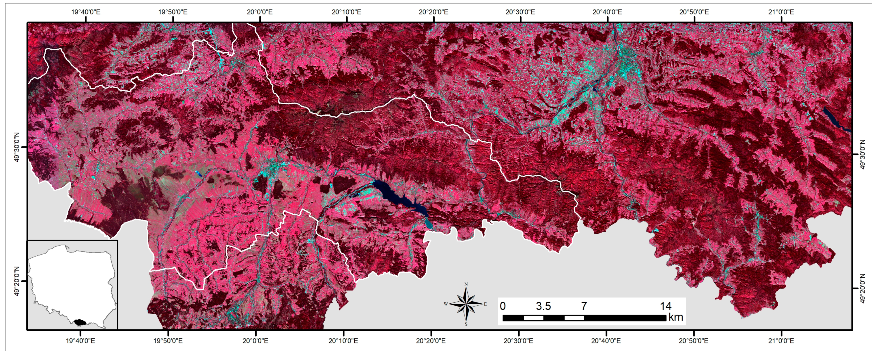
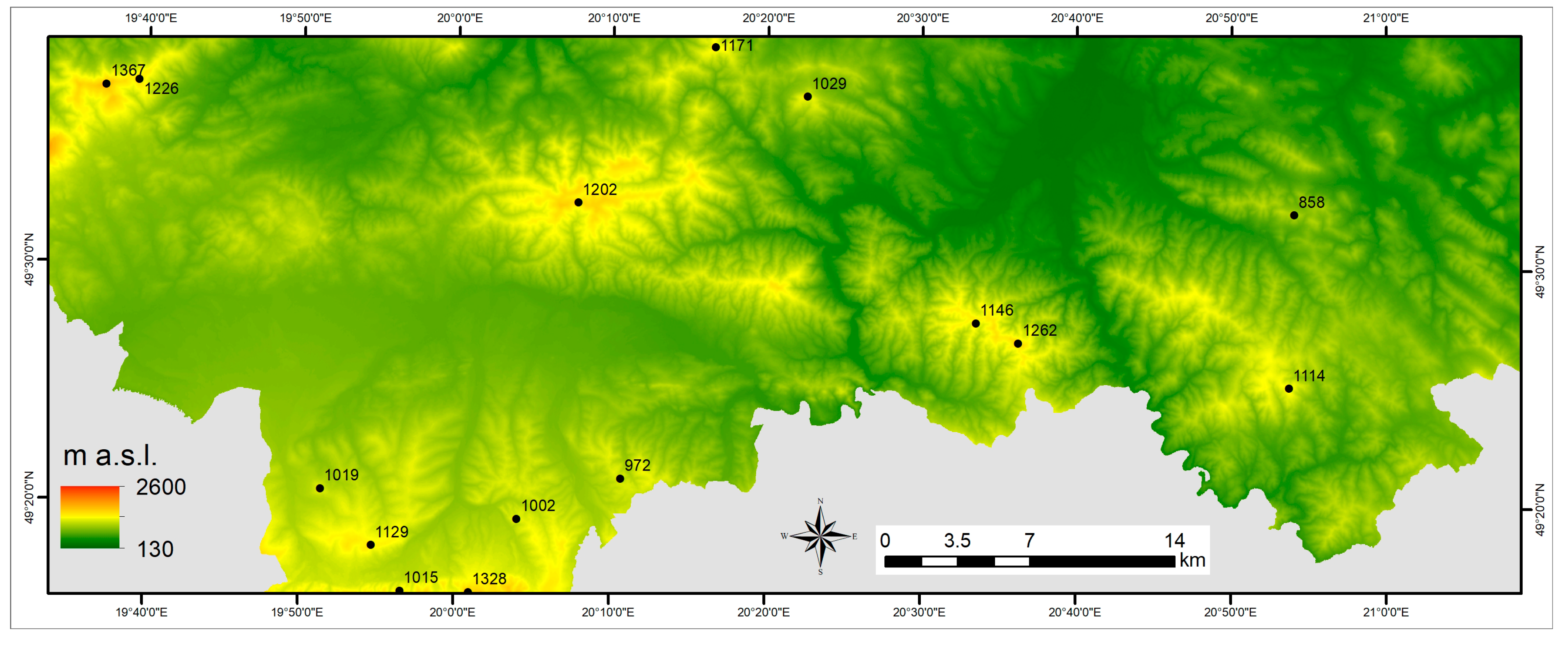
The study was conducted over an area about 380,000 ha located in southern Poland on the Slovak border (Figure 1). The south-west part of the area belongs to the Podhale region and is located in the foothills of the Tatra range of the Carpathian Mountains and the rest of the area belongs to the Beskids Mountains [37]. The terrain is a combination of plain, hilly and rounded forested mountain with the highest pick 1723 m a.s.l. (Figure 2).
The lowest zone, with the upper limit of 400–600 m a.s.l., is occupied by the riparian forest, coniferous and mixed forest with a large share of oak, beech species (Fagetum carpaticum collinum). The mountain timber lower zone up to 1250 m a.s.l. is dominated by beech, sometimes mixed with fir and spruce. The lower part of this zone is occupied by Fagetum carpaticum collinum dominated by spruce and fir forests. The upper timber zone, 1250–1550 m a.s.l. is occupied by fir, larch and spruce forest (Pineetum). The spruce forest reaches the timberline [38].
A part of the study area (147,000 ha) belongs to the Nowy Targ district, which is characterized by having one of the largest percentages of the privately owned forest in Poland. According to the General Statistical Office [39], the forest covers an area of 54,600 ha, of which 67% is privately owned. The public forest managed by the State Forests occupies 23% and the national parks occupies 6%. A large proportion of the forest is located in remote mountainous areas, which makes the forest mapping and management more complex and complicated.
2.2. Data and Data Pre-Processing
2.2.1. Sentinel-2 and DEM
A set of multispectral, cloud free Sentinel-2 data acquired in the year 2017 ± 1 was downloaded from the Copernicus Data Hub. We used four cloud-free Sentinel-2 scenes acquired in different phonological seasons: 20 April 2018, 8 August 2016, 2 October 2017 and 12 October 2018. The analyzed tree species are characterized by a different phenology [40,41], thus the satellite scenes were selected to various phases of phenology. The first image (20 April) was obtained at the beginning of spring, when broadleaf trees start to green-up; the second image (8 August) represents the mid-summer; and the third and fourth (2 October and 12 October) refer to early- and mid-autumn, when some leaves start to gradually change colors.
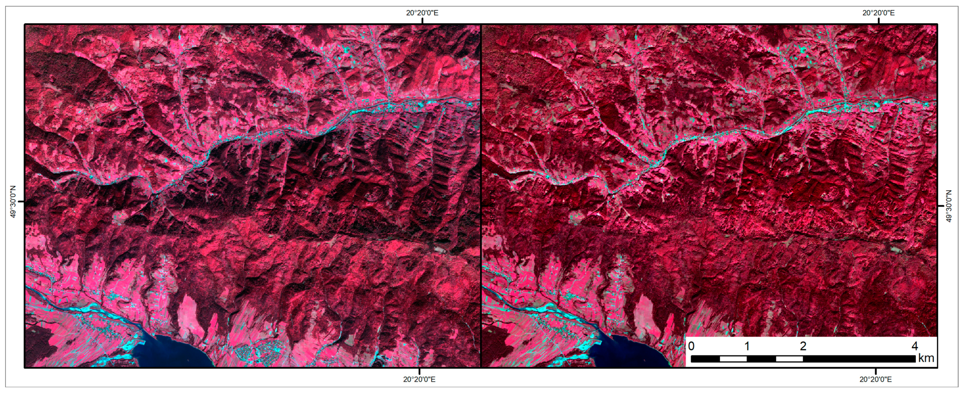
All Sentinel-2 scenes were acquired from the same orbit. The multi-spectral Sentinel-2 images Level-1C (top-of-atmosphere) orthorectified reflectance were atmospherically and topographically corrected to Level-2A (bottom-of-atmosphere) reflectance product using the Sen2Cor software, available within the Sentinel Application Platform (SNAP) provided by the European Space Agency (ESA) [42]. The algorithm used in the Sen2Cor adjusts reflectance values based on the values of sun elevation, azimuth, altitude and atmospheric parameters (i.e., visibility, aerosols, cirrus). The 90 m SRTM digital elevation database from the CGIAR-CSI available within the Sen2Cor was used to correct the topography. The algorithm performs the resampling and assembling of the DEM based on the geo locations obtained from the Level-1C metadata and creates the slope, aspect and a hill shadow map using the GDAL tools [42]. Figure 3 presents a subset of the Sentinel-2 Level-1C image acquired on 2 October 2017 and Level-2A after atmospheric and topographic correction. In this study, we used the Sentinel-2 bands available at 10 m (blue B2: 490 nm, green B3: 560 nm, red B4: 665 nm, NIR B8: 842 nm) and 20 m spatial resolutions (red-edge: B5: 705 nm, B6: 740 nm, B7: 783 nm; narrow NIR B8a: 865 nm, SWIR: B11: 1610 nm and B12: 2190 nm). All Sentinel-2 bands provided at a 20 m spatial resolution were resampled to 10 m using the nearest neighbor resampling method.
The topographic variables were derived from the Shuttle Radar Topography Mission Digital Elevation Model (SRTM DEM). This is a freely available global product delivered using radar interferometry. The SRTM is available globally at 1 arc-second at about a 30 m spatial resolution. The SRTM DEM over Poland was acquired from the USGS Earth Explorer (http://earthexplorer.usgs.gov/). The SRTM DEM was clipped to an area overlaid by the reference samples and resampled to a 10 m spatial resolution using the bilinear resampling method. The operational forest management requires the detailed information; thus, the SRTM DEM and 20 m Sentinel-2 data were resampled to a 10 m spatial resolution. Additionally, two commonly used topographic variables, slope and aspect, were derived from the SRTM DEM and added to the data stack without any adjustment.
2.2.2. Reference Data
The reference data for forest cover, type and tree species were obtained from the national forest inventory (NFI) and digital forest map (DFM). The NFI is a sampling-based inventory of the forest condition under all forms of ownership. The main aim of the NFI is to assess the state of the forest and the trends for large scale changes that occur over time [43]. The design of the sample plot grid is based on the plot configuration used in the International Co-operative Programme on Assessment and Monitoring of Air Pollution Effects on Forests (ICP Forest), operating under the Convention on Long-range Transboundary Air Pollution of the UN Economic Commission for Europe [44]. The ICP’s 16 km × 16 km grid pattern is used as a base for the NFI. For the purposes of the NFI, the grid density is increased to 4 km × 4 km. In each location, the L-shaped cluster (in which both arms of the L are of equal length) of five sampling plots located at 200 m distances from one another is established. The locations of the sampling plots are measured using the global positioning system (GPS) and are provided at a national projection. Measurements and observations are done each year on almost 20% of the sample plot clusters (5-year cycle) across the whole country. The sampling plot area depends on the features being inventoried, such as stand age and structure. Inside the larger circular sampling plots with a radius of 11.3 m (stands aged above 60 years) and 12.6 m (regeneration class stands), the standing trees with a breast-height diameter of greater than 70 mm were measured. The NFI comprises information on, for example, the forest structure, tree species composition, health status, age and presence of damage [45]. The information on the tree species composition at each sampling plot was extracted from the NFI database. The NFI sampling plots occupied by the homogenous tree species were selected for further analysis. The NFI data used in the analysis were inventoried in 2015 and 2016.
The DFM is a geometrical database with polygons representing forest compartments and stands (assigned with a unique ID) and tables of many attributes from the forest inventory that can be joined with the polygons by a unique ID. The DFM was used to extract the information on the tree species composition within each forest stand and assigned as a percentage of the stands.
The non-forest reference samples used to classify the forest and non-forest cover were selected automatically from the National Topographic Database (BDOT10k). The BDOT10k topographic database provides data with a level of detail corresponding to the topographic maps at 1:5000–1:10,000. The land cover and land use related layers were extracted from the BDOT10K database and conversed to shapefile format. In total, 637 reference non-forest samples were randomly selected over different non-woody land cover classes and were additionally checked to assure they lay on the non-woody landscape. The reference data obtained from two forest databases (Table 1) were combined in one dataset and jointly used for further analysis. First, we identified common tree species present in the study site using the NFI and DFM databases. The following eight tree species were identified for further analysis: Coniferous species—spruce (Norway spruce—Picea abies (L.) H.Karst), pine (Scots pine - Pinus sylvestris L.), fir (silver fir - Abies alba Mill.) and larch (European larch—Larix decidua Mill.)—and broadleaf species—beech (European beech—Fagus sylvatica L.), oak (English oak—Quercus robur L. and sessile oak—Quercus petraea (Matt.) Liebl.), alder (gray alder—Alnus incana (L.) Moench and black alder—Alnus glutinosa Gaertn.) and birch (silver birch—Betula pendula Roth and downy birch—Betula pubescens Ehrh.). The share of the different species for the homogenous stands according to the reference data was as follows: Spruce 30.3%, fir 28.3%, beech 24.0%, pine 11.2%, larch 2.3%, alder 1.8%, birch 0.3% and oak 0.23%.
In total, 166 homogenous NFI sampling plots, occupied mostly by spruce, pine, fir and beech species, were selected (Table 1). The center of the sampling plots was assigned as the reference sample for further analysis. In order to reduce the edge effect, manual verification against the Sentinel-2 data was done to assure that the selected NFI sampling plots were located at least 20 m from the forest edge. Furthermore, we analyzed the DFM and selected the homogenous tree species stands where one tree species occupied more than 90% of the stand. We applied an inward buffer of 20 m to minimize the edge effect at the DFM forest stands. The minimum distance between neighboring samples was greater than 20 m. In total, 1421 reference samples, representing eight tree species, were randomly selected from the tree species homogenous stands (Table 1).
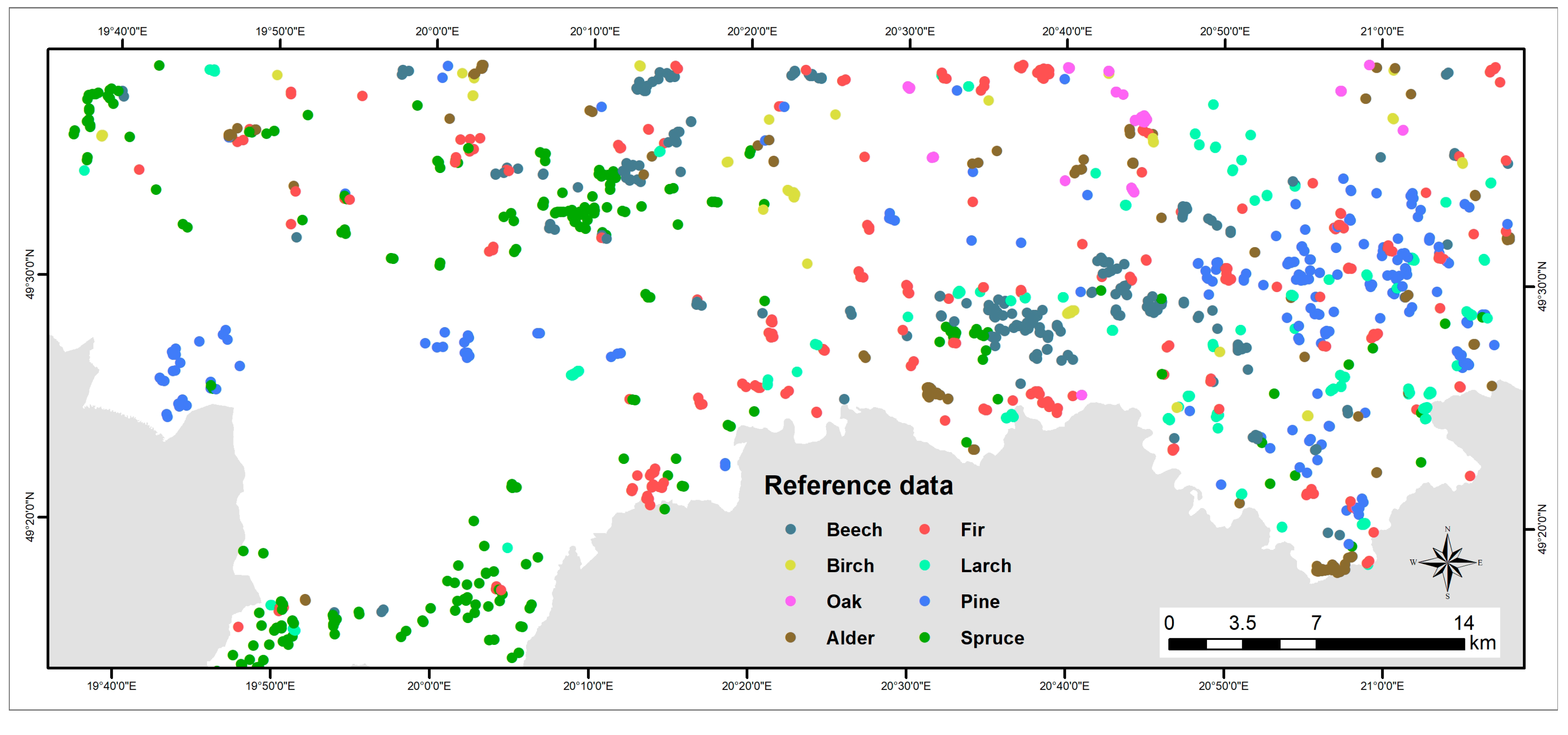
Knowing that having a high quality reference data is crucial for the machine learning algorithms, a visual verification of the reference samples was carried out using the multi-temporal Sentinel-2 images. The most frequent disagreement was observed over the spruce stands. Due to an outbreak of bark beetles, the spruce forest became very fragmented [46,47,48], and some of the randomly selected reference samples had to be moved to the remaining patches of nearby spruce forest within the homogenous spruce stand. Sometimes, the small fragments of the coniferous forest were present inside the homogenous broadleaf stands, so the reference broadleaf samples had to be moved slightly. The Sentinel-2 images acquired in different phonological seasons appeared to be very helpful in the process of visually assessing the forest type. The spatial distribution of the NFI and DFM reference samples divided into eight tree species is illustrated in Figure 4. The boxplots summarizing the distribution terrain altitude values of the individual tree species classes of reference forest data is presented in Figure 5. It is clearly visible that amongst the broadleaf forest, beech, birch and oak are dependent on the elevation, whereas the alder forest is not. This is due to the fact that alder is represented by the gray alder, which occurs mainly in the riparian zones in the mountain terrain up to 1250 m a.s.l. and the black alder, which is present at riparian zones at lowlands up to 550 m a.s.l. [49]. Amongst the coniferous forest, the spruce is highly dependent on the elevation. Of interest, out of 218 reference sample plots representing pine (Scots pine), one was located on the small patch of the mountain pine and was assigned as an extreme pine sample (Figure 5). The reference samples were randomly divided with 60% used for training and 40% for accuracy assessment purposes within the forest/non-forest, forest type and each tree species class.
2.3. Classification
The classification process was divided into three levels of forest detail: i) Mapping forest covers, ii) classification of forest type—delineation of coniferous and broadleaf forests and iii) tree species identification. We used the random forest classier for each of the three levels of analysis. The RF is a machine-learning algorithm approach that uses multiple self-learning decision trees to parameterize models and uses them to estimate variables [50,51]. The RF is an ensemble learning technique where many decision trees are constructed based on a random sub-sampling of the given data set. The advantage of RF is that it can run effectively on large and multi-source data sets and it is relatively robust to outliers, a reduction of training data and noise [50,52]. A review of the RF applications in remote sensing by Belgiu and Dragut [53] confirmed that the RF classifier is less sensitive than other streamline machine learning classifiers to the quality of training samples and to overfitting, due to the large number of decision trees produced by randomly selecting a subset of training samples and a subset of variables for splitting at each tree node. The RF classification was carried out using imagerRF [54] available at EnMAP-Box 2.2.1 developed at Humboldt-Universität zu Berlin under contract by the Helmholtz Centre Potsdam—GFZ [55]. The RF models were calibrated using 60% of the reference samples selected using the stratified random sampling. The parameterization of the model was performed on 200 single trees in the forest, the number of selected features was determined by the square root of all features, the Gini Index was used to define the impurity and minimum number of samples in a node was set to one [54,56].
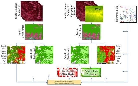
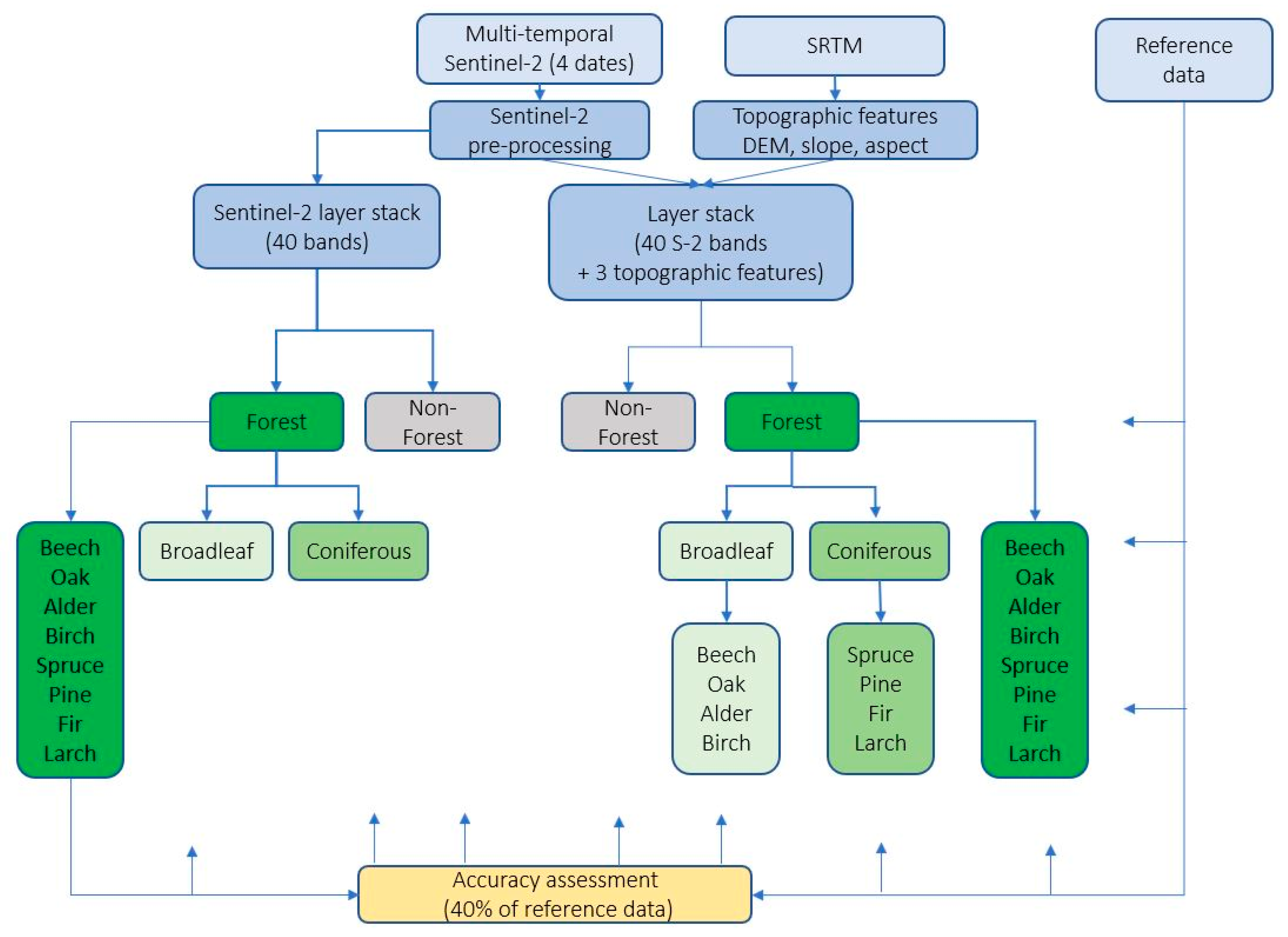
The classification performed at the three levels of forest detail used: i) Multi-temporal Sentinel-2 (10 and 20 m spatial resolution) data stack; 40 variables and ii) the combination of multi-temporal Sentinel-2 data with DEM and topographic features, such as slope and aspect, added to the data stack (43 variables). Both datasets were classified using exactly the same training sample set. The flowchart illustrating different classification scenarios is presented in Figure 6. In the first step, the forest cover was mapped then, the separation of forest types into coniferous and broadleaf was carried out inside the forest mask.
To classify the tree species, we tested two approaches. First, we classified without stratification, where eight tree species—spruce, pine, fir, larch, beech, oak, alder and birch—were classified together inside the forest mask. Second, we classified with stratification, where the broadleaf tree species were classified inside the broadleaf forest mask derived as the result of the forest type classification. An identical operation was repeated for the coniferous tree species. For both approaches, the same input variables, multi-temporal Sentinel-2 data and combination of multi-temporal Sentinel-2 and topographic information were used. We applied a similar number of reference samples for the classification of forest type and tree species. The classification models were trained based on 925 forest samples, of which 553 samples represented coniferous forest and 399 represented broadleaf forest.
In order to make the forest area comparable with the national statistics for the Nowy Targ district, we had to apply the national definition of forest. Forest, as defined in the Forest Act of 28 September 1991 [57], is a homogeneous woody area larger than 0.1 ha. This includes all forms of ownership forest and areas that are forested but officially recorded as non-forest. The woody patches lower than 0.1 ha were eliminated from the forest cover map.
2.4. Accuracy Assessment
The verification samples were selected from the reference dataset using the stratified random sampling method. The accuracy assessment was carried out individually for each classification result. The classification accuracy was expressed as the overall accuracy, kappa coefficient, the user’s and producer’s accuracy and the average F1 accuracy value. The overall accuracy is a ratio of correctly classified pixels to all verification pixels expressed as a percentage. The kappa accuracy evaluates how well the classification performs compared to randomly assigning values. The user’s accuracy (UA) is calculated as the ratio of the total number of correctly classified samples for a particular class to the total number of reference samples. The UA is a complement of the Commission Error. The producer’s accuracy (PA) refers to the ratio of accurately classified reference samples of a particular class to the total number of the reference samples for that class. The PA is a complement of the omission error. The F1 value is calculated as a weighted harmonic mean of the UA and PA. The average F1 accuracy represents the arithmetic mean of classwise F1 values. The confusion matrix presents the number of pixels that were classified into a particular class. The RF classifier in imageRF estimates the importance of variables by computing the normalized and raw variable importance. For each tree, the out-of-bag samples are permuted in the respective variable, and used to run the tree to compute the accuracies. The accuracies of the permuted out-of-bag samples are subtracted from the accuracies of the original samples. The average of the differences of the accuracies of a variable results in the raw variable importance. The normalized variable importance is calculated by dividing the raw variable importance by the respective standard deviation [56]. Generally, the most important variables for the entire RF are those with higher values of normalized variable importance.
3. Results
3.1. Forest Cover Mapping
The result of forest/non-forest classification using the random forest approach showed a high level of agreement with the forest status on the ground. The classification of the forest/non-forest cover derived from the multi-temporal Sentinel-2 data and the combination of multi-temporal Sentinel-2 and topographic features gave comparable results. The overall accuracy for both classifications was above 98%. The Kappa accuracy and F1 value were slightly higher (by 0.4%) for a combination of Sentinel-2 and topography (Table 2). The UA of forest class reached around 99% and was higher by almost 3% than the UA of the non-forest class. The PA was slightly higher (above 98%) for the forest cover class (above 97%). As the accuracy of both classifications was comparable, we used the output of the RF classification derived based on the combination of Sentinel-2 and topographic variables to calculate the forest area within the study site. Based on the results of this study, the forest covers an area of around 65,500 ha within the Nowy Targ district, which accounts for 44.4% of the district area.
3.2. Forest Type
The classification of the coniferous and broadleaf forests was carried out using two datasets: i) The multi-temporal Sentinel-2 data and ii) the combination of multi-temporal Sentinel-2 with topographic features: DEM, aspect and slope. Generally, the classification of the coniferous and broadleaf forests derived using both datasets provided high accuracy results (Table 3). In both cases, the overall accuracy was comparable and reached 94.8%, with a Kappa accuracy of 89.3% and an F1 value of 94.6%. The user’s and producer’s accuracies were also almost equal for both datasets. The coniferous forest was slightly better classified compared to the broadleaf forest. The F1 value for the classification of the coniferous forest on both datasets achieved 95.6%, whereas that of the broadleaf forest was 93.7%.
3.3. Tree Species Identification
The results of the tree species classification performed on two datasets following three classification approaches is presented in Table 4. Compared with the results of the non-stratified approach, where eight tree species (spruce, pine, fir, larch, beech, oak, alder, birch) were classified together inside the forest mask, we observed a higher accuracy for the combination of multi-temporal Sentinel-2 bands with topographic features. The overall accuracy for the combined dataset reached 81.7% and F1 was 82.4%, whereas for the multi-temporal Sentinel-2 data, the overall accuracy was equal to 75.6% and F1 was 75.7%. The evaluation of the classification performance among the individual tree species showed better results for the broadleaf species compared to the coniferous species. Four broadleaf tree species were separated with F1 accuracies above 83%. The best results were obtained for oak and beech (F1: 89.9 and 89.1%, respectively), where two and six samples were assigned to the coniferous forest, respectively. In contrast, the best separation of the coniferous tree species was obtained for pine, and fir (F1: 80.5% and 79.8%, respectively), where only one sample per class was assigned to broadleaf forest (Table 5).
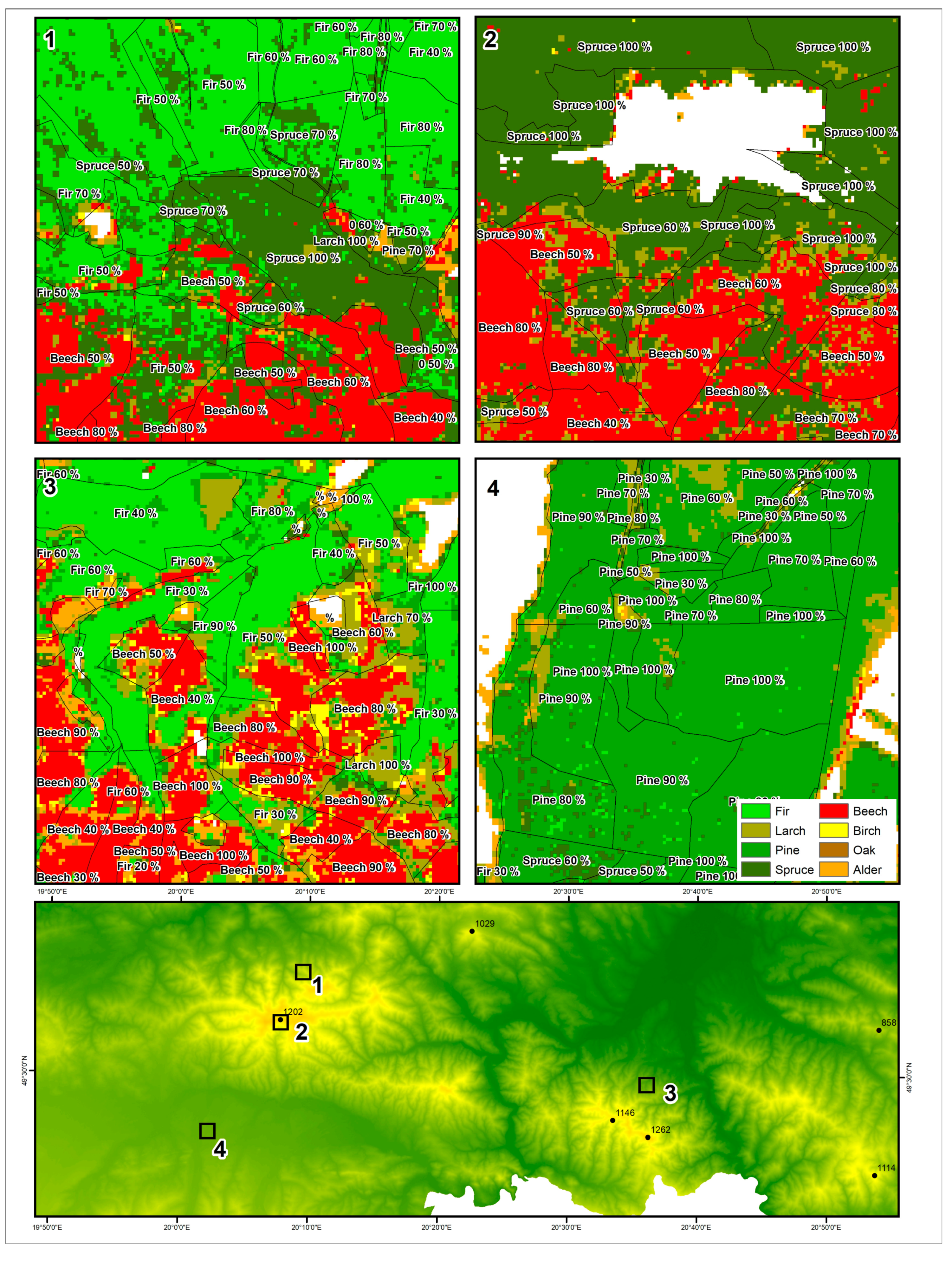
In contrast, comparing the best result of the first approach with the results of the stratified approach where the broadleaf and coniferous tree species were classified separately (each of them inside either the broadleaf or coniferous forest mask), we observed significant improvement. The overall accuracy of the stratified approach reached 89.5% for broadleaf and 82% for the coniferous species. The separation of individual broadleaf species was much better as compared with the results obtained from the first approach. The best F1 accuracy was achieved for beech (92.8%) and oak (90.7%) followed by birch (86.6%) and alder (86.3%). The classification of beech corresponds well to the information on dominant species derived from the forest stands (Figure 7). There are only seven beech samples misclassified as alder (6) and birch (1) (Table 6). We observed the overrepresentation of the alder species in the map, particularly in a form of single pixels or on the edge of the forest. In total, 14 alder’s samples (16.9%) were misclassified as other broadleaf species. The coniferous tree species performed slightly worse that the broadleaf trees. Amongst the four coniferous tree species, three of them, larch, pine and spruce, performed better in the second approach than in the first classification approach, reaching F1 values of 85.3%, 82.1% and 81.3%, respectively. The classification of spruce and Scots pine corresponded quite well to the forest stands. In the case of spruce, nine samples were confused with fir, whereas eight pine samples were misclassified as spruce (Table 6). We observed that the small patch of the mountain pine located in the northwest part of the study area was misclassified as spruce. This is probably due to the underrepresentation of the mountain pine samples in the reference dataset. In contrast, the accuracy for fir (79.8%) was comparable in both approaches. The confusion matrix for the stratified approach for all tree species is presented in Table 6. Figure 7 presents the spatial distribution of tree species derived using the stratification approach at a more detailed scale. There is a quite good agreement between the classification of tree species and species composition at the forest stand level.
3.4. Variable Importance for Tree Species Classification
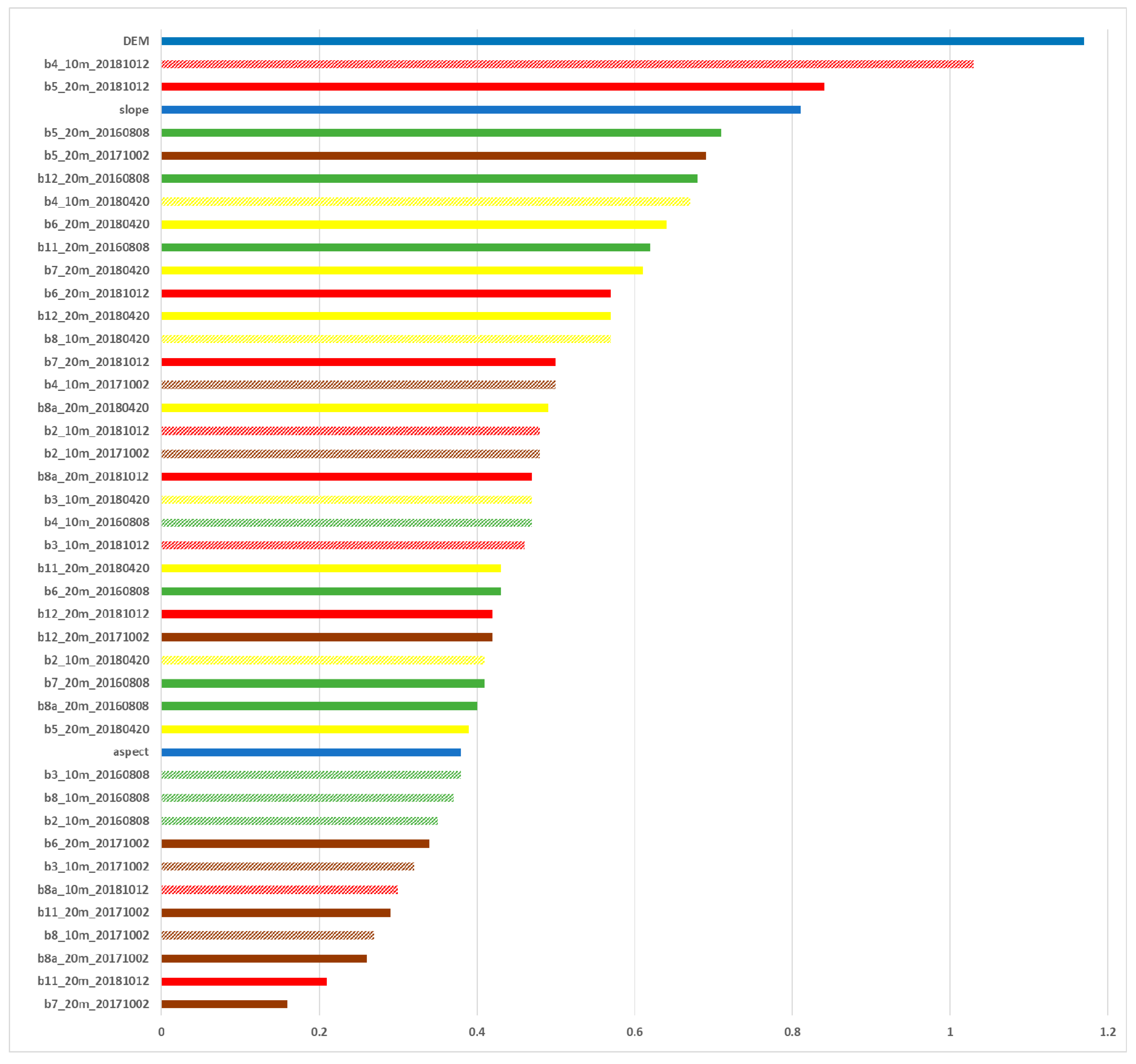
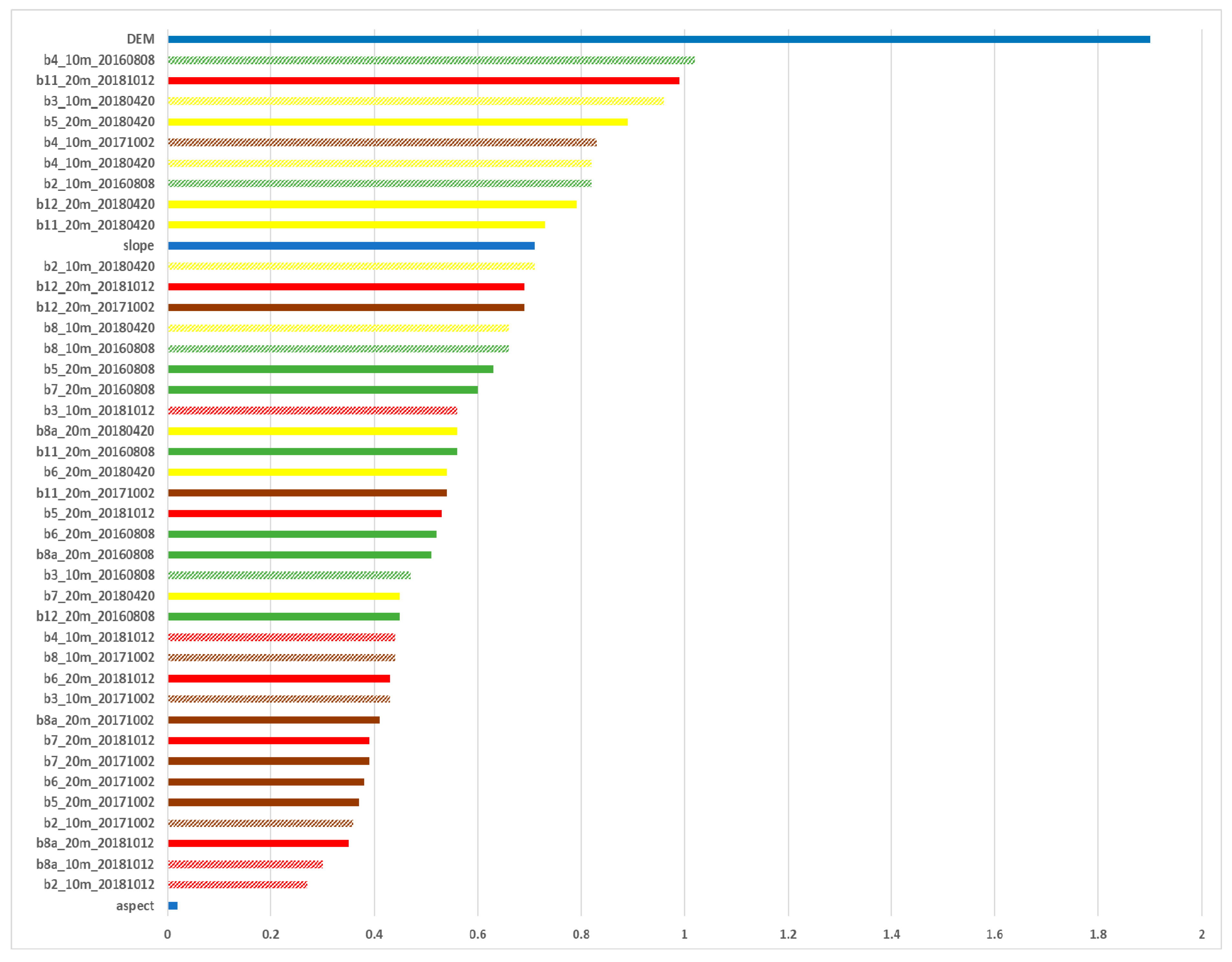
The importance of input variables in the classification of the broadleaf and coniferous tree species following the stratified approach is presented in Figure 8; Figure 9, respectively. The variables are ranked by the level of importance. The DEM contributed the most to the classification of both the broadleaf and coniferous tree species. The slope calculated from the DEM was more important for the classification of broadleaf than the coniferous tree species. The impact of aspect derived from the DEM appeared to be less important for the separation of the broadleaf tree species and not important for the delineation of the coniferous tree species. Of interest, amongst the Sentinel-2 bands, the red band (b4_10m) from 12 October (mid-autumn) and red-edge band 5 (b5_20m) acquired in autumn (12 October and 2 October) and summer (8 August) followed by SWIR bands 12 and 11 (b12_20m and b11_20m) and red-edge bands 6 and 7 contributed the most to the classification results of the broadleaf tree species. The 10 m resolution bands seemed to be less important for the separation of the broadleaf tree species; however, they were more significant for the delineation of the coniferous tree species (Figure 8). The red (b4_10m) and green (b3_10m) bands of the summer, spring and autumn Sentinel-2 images contributed the most to the result of the coniferous tree separation. Amongst the 20 m spatial resolution bands, SWIR bands 12 and 11 (b12_20m and b11_20m) derived from autumn and spring Sentinel-2 images contributed the most to the classification of coniferous tree species. Furthermore, the image acquired on 2 October was revealed to be less important in the classification of tree species, except for the red-edge band (b5_20m) for the broadleaf species and the red band (b4_10m) for the coniferous species.
4. Discussion
The study demonstrated the potential of the multi-temporal Sentinel-2 data combined with the topographic information for the operational mapping of the forest cover, forest type and detailed delineation of common tree species on a large regional scale. It has to be stressed that the number of studies focusing on forest type and tree species identification at the larger geographical scale is rather limited [35]. The wide swath of the Sentinel-2 mission, the higher spatial resolution of 10–20 m, and the revisit cycle of five days has a good basis for mapping the forest composition over large areas.
Compared to the results of other studies for classifying the forest cover, forest type and tree species, our results are comparable or more accurate. Liu et al. [26] mapped the forest cover in China applying an object-based random forest algorithm to single, multi-temporal and multi-sensed data. They achieved the highest accuracy of 99.3% by combining Sentinel-2 data with topographic information. The classification performed using only the Sentinel-2 data gave also satisfactory results of 97.2% of overall accuracy. This is in line with the results for forest cover obtained in our study. The classification of the forest and non-forest cover provided a high overall accuracy of 98.2% for multi-temporal Sentinel-2 with and without the topographic information. The overall accuracy declined slightly to 94.8% for the delineation of coniferous and broadleaf forest types. Overall, the F1 value for coniferous forest was 1.8% higher than the broadleaf forest (95.6% and 93.8%, respectively). In a study carried out in a German-managed forest (based on maximum likelihood classification (MLC) of multi-temporal Spot-4/5 and RapidEye images), Stoffels et al. [58] also achieved slightly better results for the coniferous forest (F1: 91%) compared to the broadleaf forest (F1: 90.4%). However, they achieved a lower overall accuracy of 90.7% compared to our results (94.8%).
Of interest, the use of three topographic variables—DEM, slope and aspect—did not increase the accuracy of the classification of the forest/non-forest cover and forest type (broadleaf and coniferous). In both cases, the classification results obtained with or without topographic information were comparable (Table 2 and Table 3). Our results confirmed that spectral bands derived from the multi-temporal Sentinel-2 data are sufficient to accurately map forest cover and to separate the broadleaf forest from coniferous forest over a large area. This finding was also proven by the study of Zhu and Liu [20] conducted in the second-growth forest in Vinton County, Ohio, USA. The authors concluded that the multi-temporal Landsat images are enough to distinguish broad land cover classes (including the broadleaf and coniferous forest). This research outcome should be taken into account for operational forest and forest type mapping at the regional and national scales.
In contrast, the importance of the topographic variables increased significantly in the process of tree species delineation. In our study, by combining the DEM, slope and aspect with the multi-temporal Sentinel-2 data, the classification of eight tree species improved from 75.6% (multi-temporal Sentinel-2) to 81.7% (classification without stratification, where all tree species were classified together) and reached the highest accuracy of 89.5% for the stratified approach. Liu et al. [26] demonstrated the importance of slope derived from SRTM DEM in the RF classification of four common tree species and four mixed forest types in part of China. The authors achieved the best accuracy of 82.8% by combining various spectra, textural feature derived from Sentinel-2, multi-temporal Landsat images, Sentinel-1 VV data and topographic information. The overall accuracy was approximately 13% higher compared to the classification using the combination of Sentinel-2 and topographic features (69.5%). The lower accuracy of combination of Sentinel-2 and topographic features, compared to our study, may be due to the selection of the Sentinel-2 data. Liu et al. [26] used the multi-spectral Sentinel-2 data collected in the leaf-on season only, whereas the Landsat images represented different vegetation seasons. In our study, we used four Sentinel-2 scenes representing change in phenology. According to Liu et al. [26], the DEM, followed by aspect, was listed as the least important variable. This finding is contradictory to the result of our study, where the DEM showed the highest impact on the classification of tree species, followed by slope. This disagreement could perhaps be explained by the differences in vertical zoning in the mountain forest. For example, the presence of the spruce forest is highly dependent on elevation, it is a characteristic for the upper timber zone and reaches the timberline, which may explain the high importance of the elevation in the classification of the coniferous forest. The F1 accuracy of the classification of spruce forest increased by 10.3% by adding the topographic features, this was the highest increase amongst all the analyzed tree species. The DEM demonstrated to be more important in the separation of the coniferous than broadleaf species. The dependence of the broadleaf species in particular beech, birch and oak on the elevation is visible in Figure 5. Amongst the broadleaf tree species, birch and oak showed the highest accuracy improvement of around 9.6% by combining the spectral data with the topographic features. The importance of DEM as an additional variable in the classification of forest types by a MLC classifier in steep mountainous terrains (ranging from 600 m to over 3000 m a.s.l.) in Austria was highlighted by Dorren et al. [22]. The authors improved the classification of four forest types from 64% to 73% by combining a DEM with Landsat images.
The results of our study demonstrated that the multi-seasonal images in combination with the topographic features are able to discriminate different tree species. The stratified, hierarchical approach to tree species classification examined in this study provided more accurate results compared to the non-stratified method. We first separated forest from non-forest, then divided forest into the broadleaf and coniferous forest and finally, tested whether the stratification by forest type improved the results of the tree species separation. The difference in accuracy between the two approaches was more pronounced for the broadleaf species than the coniferous species. The classification accuracy increased from 81.7% for the non-stratified approach to 89.5% for the broadleaf and 82% for the coniferous species following the stratified method. Comparing the performance of the classification of individual tree species, we obtained following the stratified approach, the highest user’s accuracy for oak (95.1%) and beech (92.3%) followed by birch (90.6%) and alder (83.1%). Wessel et al. [30] applied the stratified approach to delineate the oak and beech species in the Bavarian forest (using Sentinel-2). They first mapped the broadleaf forest, then classified the tree species within the broadleaf forest and achieved a high user accuracy of 94% for beech and 100% for oak species. Zhu et al. [20] proposed a hierarchical classification approach to classify first the broad land cover and then the detailed forest type within the broadleaf forest. They applied this approach to the Landsat time series using the SVM method and achieved the user’s accuracy of 92% for oak trees.
Our results were more accurate than those achieved using the non-stratified object-based approach based on Sentinel-2 by Immitzer et al. [32] for beech (73.8%) and oak (46.7%). The classification of tree species based on high resolution SPOT and RapidEye data by Stoffels et al. [58] also provided lower accuracy for oak (84%) and beech (79.5%). These values were more in line with the accuracy of the tree species classified together without stratification presented in our study. Lower accuracy for the classification of beech and oak (69% and 83%) using very high resolution WorldView images was also reported by Waser et al. [59]. Slightly higher user’s accuracy for beech (86.9%), oak (85.4%), birch (88.6%) and alder (79.6%) was achieved by Immitzer et al. [60] using the object-based random forest classification of the WorldView-2 satellite data in the East of Austria. Regarding the separation of coniferous tree species, the best user’s accuracy was obtained following the stratified approach for spruce (85%) and pine (84.1%), followed by larch and fir, with the user’s accuracy reaching almost 80%. The results of Stoffels et al. [58] were slightly better for spruce (91.6%) and comparable for pine and fir. The slightly lower or comparable results for spruce (80.4%), pine (85.1%), larch (70.4%), fir (82.3%) were obtained by Immitzer et al. [60]. Waser et al. [59], obtained a higher user’s accuracy for fir (85%) and larch (87%) compared to our results. Much lower accuracy was achieved based on Sentinel-2 data by Immitzer et al. [32], where spruce reached a user’s accuracy of 77%, fir 71%, larch 64% and pine 60%.
Analyzing the importance of variables used in the classification process, we observed a discrepancy between the coniferous and broadleaf tree species. The visual 10 m Sentinel-2 bands, in particularly red and green bands (B4 and B3) followed by two SWIR bands (B12 and B11), were the most important for the separation of four coniferous tree species. In contrast, the visible bands were less important in the classification of broadleaf tree species, except for the red band (B4) derived from images acquired in autumn and spring. The high relevance of the visible bands is related to the absorption of photosynthetic pigment chlorophyll a and b [35]. The red-edge bands (B5, B6 and B7) and two SWIR bands (B12 and B11) contributed the most to the results of the broadleaf tree species classification. The importance of red-edge bands in the classification of vegetation and separation of broadleaf species was highlighted by other studies [30,61]. Immitzer et al. [32] also found two SWIR (B11 and B12), one red-edge (B5) and two visible (B2, B4) bands to be the most important in the classification of six tree species. The importance of the SWIR bands (B11 and B12) in the separation of four tree species (two coniferous and two broadleaf) and four mixed forest types was also pointed out by Liu et al. [26].
The rank of the variable importance showed relatively low contributions of several spectral bands of the early autumn image (2 October); however, there were two very important spectral bands: red-edge band (B5) and red band (B4), which contributed significantly to the separation of broadleaf and coniferous species. This suggests that the phenology is the important aspect in the classification of tree species, particularly in the broadleaf forest. Since plant phenology varies with species, it is important to select images representing the phonological cycle of the studied tree species [21,62]. Changes in vegetation are most observable in spring as greening-up leaves and the intensive green color of needles and in autumn as the coloring of leaves due to leaf senescence. However, the low sun elevation angle in very early spring and late autumn images may reduce the accuracy of the classification. The terrain correction partly compensates illumination conditions for slopes facing towards or away from the sunlight but it cannot eliminate this effect completely [63]. This is particularly important for the study carried out over the complex, steep mountain areas. In our study, even the mountains were not steep, some pixels on the image acquired on the 12 October, were assigned as “dark area pixels”, which was related to the effect of the low sun elevation angle. We observed that the terrain correction improved the illumination condition over these areas. The use of the multi-temporal datasets in the areas where seasonal effect differ among the species can support the separation of the tree species and minimize illumination effects on the classification results.
It has to be highlighted that the accuracy of the classification strongly depends on the quality of the reference samples. There are a few issues to point out. First, the stand-based forest inventories provide information aggregated to the forest stand level with no information about the spatial variability of dominant tree species within the stand. Second, due to the dynamic changes of the forest status, the inventory data is not always up-to-date. In the case of our study, due to an outbreak of bark beetles, the spruce forest became very fragmented, and some of the randomly selected reference samples had to be moved to the remaining patches of nearby spruce forest within the homogenous spruce stand. Third, the information assigned to the stands can be incorrect, we observed that sometimes, the small fragments of the coniferous forest were present inside the homogenous broadleaf stands. On the other hand, with the sample-based inventories, the position of the sampling plots may be not always accurate. Therefore, the visual verification of the reference samples is essential to assure the quality of the training and validation dataset. Finally, it is important for the mountain terrain to have the reference samples covering the full elevation range for particular species. In our study, the small patch of the mountain pine was misclassified as spruce due to the underrepresentation of this species in the reference samples.
In general, the Sentinel-2 mission is perfectly designed for large-scale analysis. Due to a wide swath and dense series of the Sentinel-2 data, it is feasible to derive up-to-date forest cover and forest type maps at a high spatial resolution on an annual basis. The use of the national reference datasets, multi-temporal Sentinel-2 data and algorithms tuned to the specific area allows achieving a higher accuracy and high resolution (10 m) products compared to those currently provided by the pan-European Copernicus High Resolution Forest Layers (spatial resolution of 20 m). Additionally, the time lag in the HRL data provision is the limiting factor for the regional management purposes because it does not allow tracking the dynamic changes. However, the Copernicus High Resolution Layers are a relevant dataset for the national purposes to derive, for example, more detailed information on the land cover than those provided by the Corine Land Cover databases.
The results presented in this study demonstrate the ability to provide highly accurate, detailed and up-to-date forest maps over a large area at the regional scale. This information is crucial for local administration to improve the forest management, especially in remote areas. The Nowy Targ district is a good example for the use of the remote-sensed data in operational management processes. Knowledge on the actual forest extent can help to identify the areas with discrepancy between the official cadastre data and forest on the ground. The forest cover map derived as part of this study provides information on the actual forest extent within the district. The forest covers an area of 65,500 ha, which accounts for 44.4% of the Nowy Targ district area. This is almost 11,000 ha more than the forest area reported by official statistics [39]. Another advantage of using the Earth Observation data and techniques is that we can map and monitor forest resources, regardless of land ownership. Our study demonstrated that the satellite-based products could support traditional forest inventories by providing a large-scale wall-to-wall map of forest extent, forest type or species distribution. The final satellite-based forest cover and forest type maps are incorporated in the web-based SAT4EST application, which is designed to support the local authorities in managing and controlling the activities over the non-state forest. The application is in the pre-operational phase.
5. Conclusions
The multi-temporal freely available Sentinel-2 data acquired in different phenological phases have the potential for mapping the forest cover and forest type and delineating tree species on a large regional scale. The detailed forest cover, updated preferably on an annual basis, and forest type were identified by the local authorities as the most essential variables required for the improvement of the forest management, in particular, over remote mountain areas and in places where the traditional inventories are limited. We demonstrated that the forest cover and type could be successfully mapped at a 10 m spatial resolution with the multi-temporal Sentinel-2 data. The combination of spectral features of Sentinel-2 and topographic information did not improve the classification of forest cover and forest types. In contrast, the SRTM DEM was shown to have the highest impact on the classification of tree species. We proved that the application of the forest type stratification method to tree species identification significantly increases the overall accuracy of the classification results. The improvement of the tree species was more pronounced for broadleaved species, for which the overall classification accuracy rose from 81.7% following the non-stratified approach to 89.5% for the stratified method. The best separation of tree species, with an overall accuracy of above 85% was achieved for oak, beech, birch and spruce. Generally, the results obtained as part of this study were higher than those presented by other studies. It has to be stressed that the successful classification of tree species can be only feasible with the use of high-quality reference samples, which sometimes can be difficult to acquire. Free and open Sentinel-2 data is valuable for providing large scale monitoring of forest resources at a reasonably high spatial resolution of 10 m over large remote forest areas. One limitation of the optical Sentinel-2 data is the availability of the cloud-free images. Having more cloud-free images might improve the use of the dense multispectral satellite images. To overcome this limitation, a synergy of optical and SAR data should be examined, for forest mapping.
Author Contributions
Conceptualization, A.H.; Methodology, A.H.; Data Curation, A.L., Validation, A.H. and A.L.; Formal Analysis, A.H. and A.L.; Writing—Original Draft Preparation, A.H.; Writing—Review and Editing, A.H. and A.L.; Visualization, A.H.; Supervision, A.H.; Project Administration, A.H.
Funding
This research was funded by the European Space Agency (ESA) in the framework of the Polish Incentive Scheme program, project title: Earth observation-based service supporting local administration in non-state forest management (SAT4EST) (www.sat4est.pl).
Acknowledgments
We greatly acknowledge the Directorate-General of the State Forests for providing the forest reference data and the Head Office of Land Surveying and Cartography for providing the BDOT10K data. We also thank Bureau for Forest Management and Geodesy for access to digital forest map. We are grateful to the four anonymous reviewers for providing the constructive and valuable comments that helped us improve the manuscript.
Conflicts of Interest
The authors declare no conflict of interest.
References
- Franklin, S.E. Remote Sensing for Sustainable Forest Management; Lewis Publishers; Taylor & Francis Group, LLC: Boca Raton, FL, USA, 2001. [Google Scholar]
- UNFCCC. Kyoto Protocol Reference Manual on Accounting of Emissions and Assigned Amounts. 92-9219-055-5. 2008. Available online: https://unfccc.int/resource/docs/publications/08_unfccc_kp_ref_manual.pdf (accessed on 18 December 2018).
- IPCC. Global Warming of 1.5 °C, an IPCC Special Report on the Impacts of Global Warming of 1.5°C Above pre-Industrial Levels and Related Global Greenhouse Gas Emission Pathways, in the Context of Strengthening the Global Response to the Threat of Climate Change, Sustainable Development, and Efforts to Eradicate Poverty; World Meteorological Organization: Geneva, Switzerland, 2018. [Google Scholar]
- Naudts, K.; Chen, Y.; McGrath, M.J.; Ryder, J.; Valade, A.; Otto, J.; Luyssaert, S. Europe’s forest management did not mitigate climate warming. Science 2016, 351, 597–600. [Google Scholar] [CrossRef]
- Bengtsson, J.; Sven, G.N.; Alain, F.; Paolo, M. Biodiversity, disturbances, ecosystem function and management of European forests. For. Ecol. Manag. 2000, 132, 39–50. [Google Scholar] [CrossRef]
- Vihervaara, P.; Auvinen, A.-P.; Mononen, L.; Törmä, M.; Ahlroth, P.; Anttila, S.; Böttcher, K.; Forsius, M.; Heino, J.; Heliölä, J.; et al. How Essential Biodiversity Variables and remote sensing can help national biodiversity monitoring. Glob. Ecol. Conserv. 2017, 10, 43–59. [Google Scholar] [CrossRef]
- Proença, V.; Martin, L.J.; Pereira, H.M.; Fernandez, M.; McRae, L.; Belnap, J.; Böhm, M.; Brummitt, N.; García-Moreno, J.; Gregory, R.D.; et al. Global biodiversity monitoring: From data sources to Essential Biodiversity Variables. Biol. Conserv. 2017, 213, 256–263. [Google Scholar] [CrossRef] [Green Version]
- Bergseng, E.; Ørka, H.O.; Næsset, E.; Gobakken, T. Assessing forest inventory information obtained from different inventory approaches and remote sensing data sources. Ann. For. Sci. 2015, 75, 33–45. [Google Scholar] [CrossRef]
- GUS. Forestry 2017; Central Satatistical Office: Warsaw, Poland, 2017. Available online: https://stat.gov.pl/files/gfx/portalinformacyjny/pl/defaultaktualnosci/5510/1/13/1/lesnictwo_2017.pdf (accessed on 15 January 2019).
- Ziemblicki, M.H. Uwarunkowania prawne nadzoru nad lasami niestanowiącymi własności Skarbu Państwa/Legal conditions of supervision over private forests. Białostockie Studia Prawnicze 2015, 297–305. [Google Scholar] [CrossRef]
- Hościło, A.; Mirończuk, A.; Lewandowska, A. Określenie rzeczywistej powierzchni lasów w Polsce na podstawie dostępnych danych przestrzennych/Determination of the actual forest area in Poland based on the available spatial datasets. Sylwan 2016, 160, 627–634. [Google Scholar]
- Jabłoński, M. Powierzchnia gruntów leśnych—Przyczyny zmian i spójność źródeł danych. Wiadomości Statystyczne 2015, 11, 54–68. [Google Scholar]
- Jabłoński, M.; Mionskowski, M.; Budniak, P. Forest area in Poland based on national forest inventory. Sylwan 2018, 162, 365–372. [Google Scholar]
- Kolecka, N.; Kozak, J.; Kaim, D.; Dobosz, M.; Ginzler, C.; Psomas, A. Mapping Secondary Forest Succession on Abandoned Agricultural Land with LiDAR Point Clouds and Terrestrial Photography. Remote Sens. 2015, 7, 8300–8322. [Google Scholar] [CrossRef] [Green Version]
- Krawczyk, R. Afforestation and secondary succession. Leśne Prace Badawcze 2014, 75, 423–427. [Google Scholar] [CrossRef]
- Kolecka, N.; Kozak, J.; Kaim, D.; Dobosz, M.; Ostafin, K.; Ostapowicz, K.; Wezyk, P.; Price, B. Understanding farmland abandonment in the Polish Carpathians. Appl. Geogr. 2018, 88, 62–72. [Google Scholar] [CrossRef]
- Hansen, M.C.; Potapov, P.V.; Moore, R.; Hancher, M.; Turubanova, S.A.; Tyukavina, A.; Thau, D.; Stehman, S.V.; Goetz, S.J.; Loveland, T.R.; et al. High-Resolution Global Maps of 21st-Century Forest Cover Change. Science 2013, 342, 850–853. [Google Scholar] [CrossRef]
- Hościło, A.; Mirończuk, A.; Leszczyńska, A. The High Resolution Layer (HRL) Verification Report for Dominant Leaf Type—Poland. Unpublished Report. 2018. [Google Scholar]
- Banskota, A.; Kayastha, N.; Falkowski, M.J.; Wulder, M.A.; Froese, R.E.; White, J.C. Forest Monitoring Using Landsat Time Series Data: A Review. Can. J. Remote Sens. 2014, 40, 362–384. [Google Scholar] [CrossRef]
- Zhu, X.; Liu, D. Accurate mapping of forest types using dense seasonal Landsat time-series. ISPRS J. Photogramm. Remote Sens. 2014, 96, 1–11. [Google Scholar] [CrossRef]
- Gärtner, P.; Förster, M.; Kleinschmit, B. The benefit of synthetically generated RapidEye and Landsat 8 data fusion time series for riparian forest disturbance monitoring. Remote Sens. Environ. 2016, 177, 237–247. [Google Scholar] [CrossRef] [Green Version]
- Dorren, L.K.A.; Maier, B.; Seijmonsbergen, A.C. Improved Landsat-based forest mapping in steep mountainous terrain using object-based classification. For. Ecol. Manag. 2003, 183, 31–46. [Google Scholar] [CrossRef]
- Pasquarella, V.J.; Holden, C.E.; Woodcock, C.E. Improved mapping of forest type using spectral-temporal Landsat features. Remote Sens. Environ. 2018, 210, 193–207. [Google Scholar] [CrossRef]
- Ji, W.; Wang, L. Phenology-guided saltcedar (Tamarix spp.) mapping using Landsat TM images in western U.S. Remote Sens. Environ. 2016, 173, 29–38. [Google Scholar] [CrossRef]
- Castillo, E.M.D.; García-Martin, A.; Aladren, L.A.L.; Luis, M.D. Evaluation of forest cover change using remote sensing techniquesand landscape metrics in Moncayo Natural Park (Spain). Appl. Geogr. 2015, 62, 247–255. [Google Scholar] [CrossRef]
- Liu, Y.A.; Gong, W.S.; Hu, X.Y.; Gong, J.Y. Forest Type Identification with Random Forest Using Sentinel-1A, Sentinel-2A, Multi-Temporal Landsat-8 and DEM Data. Remote Sens. 2018, 10, 946. [Google Scholar] [CrossRef]
- Sheeren, D.; Fauvel, M.; Josipović, V.; Lopes, M.; Planque, C.; Willm, J.; Dejoux, J.-F. Tree Species Classification in Temperate Forests Using Formosat-2 Satellite Image Time Series. Remote Sens. 2016, 8, 734. [Google Scholar] [CrossRef]
- ESA. Sentinel-2 User Handbook. 2015. Available online: https://sentinel.esa.int/documents/247904/685211/Sentinel-2_User_Handbook (accessed on 10 January 2018).
- Escobar-Flores, J.G.; Lopez-Sanchez, C.A.; Sandoval, S.; Marquez-Linares, M.A.; Wehenkel, C. Predicting Pinus monophylla forest cover in the Baja California Desert by remote sensing. Peerj 2018, 6, 1–17. [Google Scholar] [CrossRef] [PubMed]
- Wessel, M.; Brandmeier, M.; Tiede, D. Evaluation of Different Machine Learning Algorithms for Scalable Classification of Tree Types and Tree Species Based on Sentinel-2 Data. Remote Sens. 2018, 10, 1419. [Google Scholar] [CrossRef]
- Puletti, N.; Chianucci, F.; Castaldi, C. Use of Sentinel-2 for forest classification in Mediterranean environments. Ann. Silvic. Res. 2018, 42, 32–38. [Google Scholar] [CrossRef]
- Immitzer, M.; Vuolo, F.; Atzberger, C. First Experience with Sentinel-2 Data for Crop and Tree Species Classifications in Central Europe. Remote Sens. 2016, 8, 166. [Google Scholar] [CrossRef]
- Wittke, S.; Yu, X.; Karjalainen, M.; Hyyppä, J.; Puttonen, E. Comparison of two-dimensional multitemporal Sentinel-2 data with three-dimensional remote sensing data sources for forest inventory parameter estimation over a boreal forest. Int. J. Appl. Earth Obs. Geoinf. 2019, 76, 167–178. [Google Scholar] [CrossRef]
- Persson, M.; Lindberg, E.; Reese, H. Tree Species Classification with Multi-Temporal Sentinel-2 Data. Remote Sens. 2018, 10, 1794. [Google Scholar] [CrossRef]
- Fassnacht, F.E.; Latifi, H.; Stereńczak, K.; Modzelewska, A.; Lefsky, M.; Waser, L.T.; Straub, C.; Ghosh, A. Review of studies on tree species classification from remotely sensed data. Remote Sens. Environ. 2016, 186, 64–87. [Google Scholar] [CrossRef]
- Isuhuaylas, L.A.V.; Hirata, Y.; Santos, L.C.V.; Torobeo, N.S. Natural Forest Mapping in the Andes (Peru): A Comparison of the Performance of Machine-Learning Algorithms. Remote Sens. 2018, 10, 782. [Google Scholar] [CrossRef]
- Kondracki, J. Geografia Regionalna Polski; PWN: Warszawa, Poland, 2002. [Google Scholar]
- Szymański, S. Ekologiczne Podstawy Hodowli Lasu; PWN: Warszawa, Poland, 2000. [Google Scholar]
- GUS. Local Data Bank. 2017. Available online: https://bdl.stat.gov.pl/ (accessed on 10 December 2018).
- Schieber, B.; Kubov, M.; Janik, R. Effects of Climate Warming on Vegetative Phenology of the Common Beech Fagus sylvatica in a Submontane Forest of the Western Carpathians: TwoDecade Analysis. Pol. J. Ecol. 2017, 65, 339–351. [Google Scholar] [CrossRef]
- Jabłońska, K.; Kwiatkowska-Falińska, A.; Czernecki, B.; Walawender, J.P. Changes in spring and summer phenology in Poland—Responses of selected plant species to air temperature variations. Pol. J. Ecol. 2015, 63, 311–319. [Google Scholar] [CrossRef]
- Sen2Cor. STEP Science Toolbox Exploitation Platform. Available online: http://step.esa.int/main/third-party-plugins-2/sen2cor/ (accessed on 20 April 2018).
- BULiGL. The National Forest Inventory, Results of Cycle II (2012-2014) (Wielkoobszarowa Inwentaryzacja Stanu Lasów—Wyniki II Cyklu, Lata 2010–2014); Oficyna Wydawnicza FOREST, Ed.; Biuro Urządzania Lasu i Gospodarki Leśnej: Sękoci Stary, Poland, 2015. [Google Scholar]
- Michel, A.; Seidling, W. Forest Condition in Europe: 2017 Technical Report of ICP Forests. Report under the UNECE Convention on Long-Range Transboundary Air Pollution (CLRTAP); Michel, A., Seidling, W., Eds.; BFW-Dokumentation 24/2017; BFW Austrian Research Centre for Forests: Vienna, Austria, 2017; p. 123. [Google Scholar]
- BULiGL. Wieloobszarowa Inwentaryzacja Stanu Lasu w Polsce Wyniki za Okres 2013–2017; BULiGL: Sękocin Stary, Poland, 2018. [Google Scholar]
- Grodzki, W.; Fronek, W.G. Effect of forest protection strategy on the occurrence of the spruce bark beetle Ips typographus (L.) in the Kogcieliska Valley in the Tatra National Park. Sylwan 2018, 162, 628–637. [Google Scholar]
- Potterf, M.; Nikolov, C.; Kocicka, E.; Ferencik, J.; Mezei, P.; Jakus, R. Landscape-level spread of beetle infestations from windthrown- and beetle-killed trees in the non-intervention zone of the Tatra National Park, Slovakia (Central Europe). For. Ecol. Manag. 2019, 432, 489–500. [Google Scholar] [CrossRef]
- Fleischer, P.; Koren, M.; Skvarenina, J.; Kunca, V. Risk Assessment of the Tatra Mountains Forest; Springer Science+Buisness Media: New York, NY, USA, 2009. [Google Scholar] [CrossRef]
- Danielewicz, W. Encyklopedia Leśna. In Encyklopedia Leśna; Ośrodek Rozwojowo-Wdrożeniowy Lasów Państwowych w Bedoniu: Nowy Bedoń, Poland, 2018; Available online: https://www.encyklopedialesna.pl/ (accessed on 12 January 2019).
- Breiman, L. Random Forests. Mach. Learn. 2001, 45, 5–32. [Google Scholar] [CrossRef] [Green Version]
- Hastie, T.; Tibshirani, R.; Friedman, J. The Elements of Statistical Learning. Data Mining, Inference, and Prediction; Springer Science+Buisness Media: New York, NY, USA, 2009. [Google Scholar] [CrossRef]
- Rodriguez-Galiano, V.F.; Ghimire, B.; Rogan, J.; Chica-Olmo, M.; Rigol-Sanchez, J.P. An assessment of the effectiveness of a random forest classifier for land-cover classification. ISPRS J. Photogramm. Remote Sens. 2012, 67, 93–104. [Google Scholar] [CrossRef]
- Belgiu, M.; Dragut, L. Random forest in remote sensing: A review of applications and future directions. ISPRS J. Photogramm. Remote Sens. 2016, 114, 24–31. [Google Scholar] [CrossRef]
- Waske, B.; Linden, S.v.d.; Oldenburg, C.; Jakimow, B.; Rabe, A.; Hostert, P. imageRFeA user-oriented implementation for remote sensing image analysiswith Random Forests. Environ. Model. Softw. 2012, 35, 192–193. [Google Scholar] [CrossRef]
- Van der Linden, S.; Rabe, A.; Held, M.; Jakimow, B.; Leitão, P.J.; Okujeni, A.; Schwieder, M.; Suess, S.; Hostert, P. The EnMAP-Box—A Toolbox and Application Programming Interface for EnMAP Data Processing. Remote Sens. 2015, 7, 11249–11266. [Google Scholar] [CrossRef] [Green Version]
- Jakimow, B.; Oldenburg, C.; Rabe, A.; Waske, B.; van der Linden, S.; Hostert, P. Manual for Application: imageRF (1.1); Universität Bonn, Institute of Geodesy and Geo Information, Department of Photogrammetry and Humboldt-Universität zu Berlin, Geomatics Lab.: Berlin, Germany, 2012. [Google Scholar]
- Act, F. Forest Act of 28 September 1991/Ustawa o Lasach z Dnia 28 Września 1991 r. Dz. U. 1991, 101. [Google Scholar]
- Stoffels, J.; Hill, J.; Sachtleber, T.; Mader, S.; Buddenbaum, H.; Stern, O.; Langshausen, J.; Dietz, J.; Ontrup, G. Satellite-Based Derivation of High-Resolution Forest Information Layers for Operational Forest Management. Forests 2015, 6, 1982. [Google Scholar] [CrossRef]
- Waser, L.T.; Küchler, M.; Jütte, K.; Stampfer, T. Evaluating the Potential of WorldView-2 Data to Classify Tree Species and Different Levels of Ash Mortality. Remote Sens. 2014, 6, 4515–4545. [Google Scholar] [CrossRef] [Green Version]
- Immitzer, M.; Atzberger, C.; Koukal, T. Tree Species Classification with Random Forest Using Very High Spatial Resolution 8-Band WorldView-2 Satellite Data. Remote Sens. 2012, 4, 2661–2693. [Google Scholar] [CrossRef] [Green Version]
- Schuster, C.; Förster, M.; Kleinschmit, B. Testing the red edge channel for improving land-use classifications based on high-resolution multi-spectral satellite data. Int. J. Remote Sens. 2012, 33, 5583–5599. [Google Scholar] [CrossRef]
- Hill, R.A.; Wilson, A.K.; George, M.; Hinsley, S.A. Mapping tree species in temperate deciduous woodland using time-series multi-spectral data. Appl. Veg. Sci. 2010, 13, 86–99. [Google Scholar] [CrossRef]
- Meyer, P.; Itten, K.I.; Kellenberger, T.; Sandmeier, S.; Sandmeier, R. Radiometric corrections of topographically induced effects on Landsat TM data in an alpine environment. ISPRS J. Photogramm. Remote Sens. 1993, 48, 17–28. [Google Scholar] [CrossRef]
Figure 1.
Location of the study site. The color composite of Sentinel-2 from 2 October 2017 (bands 8, 4 and 3) with outline of the border of the Nowy Targ district.
Figure 1.
Location of the study site. The color composite of Sentinel-2 from 2 October 2017 (bands 8, 4 and 3) with outline of the border of the Nowy Targ district.

Figure 2.
Shuttle Radar Topography Mission Digital Elevation Model (SRTM DEM) of the study area.

Figure 3.
A subset of the Sentinel-2 image acquired on 2 October 2017 (band combination 8, 4 and 3), on the left: Level-1C—before and on the right: Level 2A after atmospheric and topographic correction.
Figure 3.
A subset of the Sentinel-2 image acquired on 2 October 2017 (band combination 8, 4 and 3), on the left: Level-1C—before and on the right: Level 2A after atmospheric and topographic correction.

Figure 4.
Locations of the reference samples coloured by tree species.

Figure 5.
Distribution of terrain altitude values of the classes of the individual tree species.

Figure 6.
Flowchart of the applied methods for forest/non-forest cover, forest type and species mapping.
Figure 6.
Flowchart of the applied methods for forest/non-forest cover, forest type and species mapping.

Figure 7.
Fragment of the tree species map derived using the stratification approach based on the multi-temporal Sentinel-2 data combined with topographic features with overlaid forest stands with information on the dominant tree species and percentage of it within the stand. The bottom map shows the exact extend and location of the subsets presented above overlaid on the SRTM DEM.

Figure 8.
The normalised variable importance for broadleaf tree species classified using the combination of multi-temporal Sentinel-2 data and topographic features: DEM, slope and aspect. The variables are coloured according the Sentinel-2 acquisitions: Yellow indicates Spring (20 April), green—Summer (8 August), brown—early Autumn (2 October), red—mid-Autumn (12 October) and blue indicates the topographic features. The solid colours refer to 10 m spatial resolution bands and the dash pattern refers to 20 m spatial resolution bands.

Figure 9.
The normalised variable importance for the coniferous tree species classified using the combination of multi-temporal Sentinel-2 data and topographic features: SRTM DEM, slope and aspect. The variables are coloured according the Sentinel-2 acquisitions: Yellow indicates Spring (20 April), green—Summer (8 August), brown—early Autumn (2 October), red—mid-Autumn (12 October) and blue indicates topographic features. The solid colours refer to 10 m spatial resolution bands and the dash pattern refers to 20 m spatial resolution bands.


Table 1.
The number of reference samples used for forest type and tree species classification.
| Forest Type | Common Tree Species | National Forest Inventory (NFI) | Digital Forest Map (DFM) | Total |
|---|---|---|---|---|
| Coniferous | Spruce | 54 | 196 | 250 |
| Pine | 17 | 201 | 218 | |
| Fir | 51 | 200 | 251 | |
| Larch | 3 | 200 | 203 | |
| Broadleaf | Beech | 34 | 200 | 234 |
| Oak | 2 | 111 | 113 | |
| Alder | 2 | 200 | 202 | |
| Birch | 3 | 113 | 116 | |
| Total | 166 | 1421 | 1587 |
Table 2.
The summary of the accuracy assessment for the forest/non-forest classification.
| Sentinel-2 | Sentinel-2 + Topography 1 | |||
|---|---|---|---|---|
| Forest type | Forest | Non-Forest | Forest | Non-Forest |
| UA (%) | 98.92 | 96.37 | 99.13 | 96.39 |
| PA (%) | 98.49 | 97.38 | 98.49 | 97.82 |
| F1 (%) | 98.70 | 96.88 | 98.81 | 97.14 |
| Overall Accuracy | 98.17 | 98.32 | ||
| Kappa Accuracy | 95.58 | 95.95 | ||
| Avg. F1 Accuracy | 97.79 | 98.06 | ||
1 Topography refers to DEM, slope and aspect, UA = user’s accuracy; PA = producer’s accuracy; F1 = Avg. F1 Accuracy.
Table 3.
The accuracy of the classification of coniferous and broadleaf forests.
| Forest type | Sentinel-2 | Sentinel-2 + Topography | ||
|---|---|---|---|---|
| Coniferous | Broadleaf | Coniferous | Broadleaf | |
| UA (%) | 96.46 | 92.54 | 96.21 | 92.86 |
| PA (%) | 94.65 | 95.02 | 94.92 | 94.64 |
| F1 | 95.55 | 93.76 | 95.56 | 93.74 |
| Overall Accuracy | 94.80 | 94.80 | ||
| Kappa Accuracy | 89.31 | 89.30 | ||
| Avg. F1 Accuracy | 94.65 | 94.65 | ||
Table 4.
Accuracy assessment for different tree species classification scenarios.
| Sentinel-2 | Sentinel-2 + Topography | Sentinel-2 + Topography with Stratification | |||||||
|---|---|---|---|---|---|---|---|---|---|
| Tree species | UA % | PA % | F1 % | UA % | PA % | F1 % | UA % | PA % | F1 % |
| Beech | 85.57 | 88.30 | 86.91 | 86.87 | 91.49 | 89.12 | 92.31 | 93.33 | 92.82 |
| Birch | 81.82 | 67.50 | 73.97 | 91.18 | 77.50 | 83.78 | 90.63 | 82.86 | 86.57 |
| Oak | 80.43 | 80.43 | 80.43 | 93.02 | 86.96 | 89.89 | 95.12 | 86.67 | 90.70 |
| Alder | 71.43 | 80.25 | 75.58 | 81.93 | 83.95 | 82.93 | 83.13 | 89.61 | 86.25 |
| Fir | 82.02 | 70.87 | 76.04 | 79.05 | 80.58 | 79.81 | 79.41 | 80.20 | 79.80 |
| Larch | 68.32 | 84.15 | 75.41 | 68.27 | 86.59 | 76.34 | 79.76 | 91.78 | 85.35 |
| Pine | 73.17 | 68.97 | 71.01 | 82.93 | 78.16 | 80.47 | 84.15 | 80.23 | 82.14 |
| Spruce | 68.75 | 64.71 | 66.67 | 84.71 | 70.59 | 77.01 | 85.06 | 77.89 | 81.32 |
| OverallAccuracy % | 75.59 | 81.73 | Broadleaf | 89.47 | |||||
| Coniferous | 81.97 | ||||||||
| Kappaaccuracy % | 71.79 | 78.88 | Broadleaf | 85.22 | |||||
| Coniferous | 75.90 | ||||||||
| Avg. F1 Accuracy % | 75.75 | 82.42 | Broadleaf | 89.08 | |||||
| Coniferous | 82.15 | ||||||||
Table 5.
Confusion matrix for the approach without stratification, where all eight-tree species (beech, oak, alder, birch and spruce, pine, fir, larch) were classified together inside the forest mask using the combination of multi-temporal Sentinel-2 and topographic features.
Table 5.
Confusion matrix for the approach without stratification, where all eight-tree species (beech, oak, alder, birch and spruce, pine, fir, larch) were classified together inside the forest mask using the combination of multi-temporal Sentinel-2 and topographic features.
| Without Stratification | Beech | Birch | Oak | Alder | Fir | Larch | Pine | Spruce |
|---|---|---|---|---|---|---|---|---|
| Beech | 86 | 1 | 0 | 6 | 0 | 2 | 0 | 4 |
| Birch | 0 | 31 | 2 | 1 | 0 | 0 | 0 | 0 |
| Oak | 0 | 1 | 40 | 0 | 0 | 0 | 0 | 2 |
| Alder | 3 | 1 | 3 | 68 | 2 | 3 | 1 | 2 |
| Fir | 1 | 0 | 0 | 0 | 83 | 1 | 9 | 11 |
| Larch | 3 | 6 | 1 | 5 | 8 | 71 | 6 | 4 |
| Pine | 0 | 0 | 0 | 1 | 2 | 4 | 68 | 7 |
| Spruce | 1 | 0 | 0 | 0 | 8 | 1 | 3 | 72 |
Table 6.
Confusion matrix for the stratified approach based on combination of multi-temporal Sentinel-2 and topographic features, where broadleaf tree species and coniferous tree species were classified separately, each of them inside either broadleaf or coniferous forest masks.
Table 6.
Confusion matrix for the stratified approach based on combination of multi-temporal Sentinel-2 and topographic features, where broadleaf tree species and coniferous tree species were classified separately, each of them inside either broadleaf or coniferous forest masks.
| With Stratification | Beech | Birch | Oak | Alder | Fir | Larch | Pine | Spruce | |
|---|---|---|---|---|---|---|---|---|---|
| Beech | 84 | 1 | 0 | 6 | Fir | 81 | 1 | 9 | 11 |
| Birch | 0 | 29 | 2 | 1 | Larch | 9 | 67 | 6 | 2 |
| Oak | 0 | 1 | 39 | 1 | Pine | 2 | 3 | 69 | 8 |
| Alder | 6 | 4 | 4 | 69 | Spruce | 9 | 2 | 2 | 74 |
© 2019 by the authors. Licensee MDPI, Basel, Switzerland. This article is an open access article distributed under the terms and conditions of the Creative Commons Attribution (CC BY) license (http://creativecommons.org/licenses/by/4.0/).
Share and Cite
MDPI and ACS Style
Hościło, A.; Lewandowska, A. Mapping Forest Type and Tree Species on a Regional Scale Using Multi-Temporal Sentinel-2 Data. Remote Sens. 2019, 11, 929. https://doi.org/10.3390/rs11080929
AMA Style
Hościło A, Lewandowska A. Mapping Forest Type and Tree Species on a Regional Scale Using Multi-Temporal Sentinel-2 Data. Remote Sensing. 2019; 11(8):929. https://doi.org/10.3390/rs11080929
Chicago/Turabian StyleHościło, Agata, and Aneta Lewandowska. 2019. "Mapping Forest Type and Tree Species on a Regional Scale Using Multi-Temporal Sentinel-2 Data" Remote Sensing 11, no. 8: 929. https://doi.org/10.3390/rs11080929
Note that from the first issue of 2016, this journal uses article numbers instead of page numbers. See further details here.