Simulation and Analysis of Photogrammetric UAV Image Blocks—Influence of Camera Calibration Error


LaSTIG, IGN, ENSG, University Paris-Est, F-94160 Saint-Mande, France
*
Authors to whom correspondence should be addressed.
Remote Sens. 2020, 12(1), 22; https://doi.org/10.3390/rs12010022
Submission received: 1 October 2019
/
Revised: 10 December 2019
/
Accepted: 10 December 2019
/
Published: 19 December 2019
(This article belongs to the Special Issue Unmanned Aerial Vehicles in Geomatics)
Abstract
:Unmanned aerial vehicles (UAV) are increasingly used for topographic mapping. The camera calibration for UAV image blocks can be performed a priori or during the bundle block adjustment (self-calibration). For an area of interest with flat scene and corridor configuration, the focal length of camera is highly correlated with the height of the camera. Furthermore, systematic errors of camera calibration accumulate on the longer dimension and cause deformation. Therefore, special precautions must be taken when estimating camera calibration parameters. In order to better investigate the impact of camera calibration errors, a synthetic, error-free aerial image block is generated to simulate several issues of interest. Firstly, the erroneous focal length in the case of camera pre-calibration is studied. Nadir images are not able to prevent camera poses from drifting to compensate for the erroneous focal length, whereas the inclusion of oblique images brings significant improvement. Secondly, the case where the focal length varies gradually (e.g., when the camera subject to temperature changes) is investigated. The neglect of this phenomenon can substantially degrade the 3D measurement accuracy. Different flight configurations and flight orders are analyzed, the combination of oblique and nadir images shows better performance. At last, the rolling shutter effect is investigated. The influence of camera rotational motion on the final accuracy is negligible compared to that of the translational motion. The acquisition configurations investigated are not able to mitigate the degradation introduced by the rolling shutter effect. Other solutions such as correcting image measurements or including camera motion parameters in the bundle block adjustment should be exploited.
1. Introduction
The derivation of geospatial information from unmanned aerial vehicles (UAV) is becoming increasingly ubiquitous [1]. By applying proper processing, the image pose can be derived from aerial images with high accuracy. The bundle block adjustment (BBA) is a basic tool for photogrammetric pose estimation. In essence, the procedure consists of identifying common feature points between overlapping images and recovering their poses (i.e., positions and orientations) at first in a relative coordinate system, followed by the georeferencing phase with the help of, for example, ground control points (GCP) or the camera positions measured with global navigation satellite system (GNSS) [2,3]. Camera calibration parameters can be considered pre-calibrated and constant, or their values can be re-estimated in the self-calibrating bundle block adjustment [4,5].
In corridor mapping scenarios, continuously overlapping images are taken in series. Unlike block configuration, it constitutes only few parallel strips and cross strips are often absent. This unfavourable configuration makes the camera self-calibration less accurate. Moreover, the lack of difference in altitude introduces correlations between the interior and exterior orientation parameters, especially in the vertical direction.
Various investigations have been carried out on the systematic errors in 3D measurements and strategies have been proposed for systematic error mitigation. A first focus is given to different camera calibration models. One category consists of physical models which mitigate systematic errors according to their assumed physical behavior [6,7,8]. In the other category, individual error sources are not explicitly treated. Instead, numerical models are designed to compensate for the total systematic errors [9,10].
The magnitude of systematic errors is also influenced by camera specifications (sensor format, lens focal length, etc.). The majority of commercially available cameras for UAV surveys are not designed explicitly for photogrammetric acquisitions. Consumer-grade cameras are a popular choice because of their light weight and low cost. However, they exhibit much greater distortion and instability [11,12,13]. Zoom lenses are used in certain studies [14]; however, a fixed focal length prime lens is more likely to provide a stable performance [11].
The camera calibration can be performed with two strategies: it can either be performed independently of aerial acquisitions (pre-calibration) or be included in the bundle block adjustment (self-calibration). The pre-calibration is often performed in-lab using convergent images and varying scene depth. Lichti indicated that the laboratory camera calibration still has issues in the context of aerial photogrammetry since the depth of the calibration scene and the acquisition scene do not vary within the same scale [15]. An aerial approach is then proposed for better camera calibration. The self-calibration profits from the advances in automated feature identification and matching in recent years. There is a risk that the distortion parameters derived in this way are specific to the dataset and may not be applicable to other image sets. Comprised acquisition configurations such as nadir images in strips and blocks, result in poorly-modelled camera calibration and model deformation [12,13,16,17].
Therefore, attentions have also been directed towards camera networks. Research showed that 3D reconstructions conducted with nadir images often consist of systematic broad-scale deformations, expressed as a central doming [16,18]. The use of oblique perspectives, though more complex to perform, is proved to be an effective solution to the systematic error mitigation [19,20,21]. Wackrow studied the acquisition configuration with both simulation and practical datasets, an oblique convergent image configuration was proposed as a new approach to increasing the accuracy of 3D measurements [22]. James used simulations of multi-image networks and demonstrated the doming effect under different viewing configurations [17]. Though extensive research has been conducted on camera networks for the mitigation of systematic errors, experiences are often taken under generic conditions. How camera networks impact the modeling accuracy in specific acquisition conditions is less addressed. Our findings pay interests in the impact of camera networks on camera calibration errors and the final reconstruction accuracy.
In this article, three issues of corridor aerial image block are investigated: an erroneous focal length in camera pre-calibration; a gradually varied focal length due to camera temperature change; and the rolling shutter effect for consumer-grade cameras. For each matter, different camera viewing configurations, different flight orders and their impact on the modeling accuracy are studied. To avoid the potential perturbation introduced by other errors than that of interest, we generate a synthetic, error-free aerial image block which is of flat, corridor configuration. The addressed problems are then simulated basing on the synthetic dataset and thorough investigations are conducted. The synthetic dataset makes it possible to focus on one issue at a time while obviating the influence introduced by other types of error.
2. Data Generation and Research Design
2.1. Generation of a Synthetic Dataset
To generate a synthetic, error-free dataset, a real aerial image block was employed. In this way, the tie point multiplicity and distribution, as well as the image overlapping, were ensured to be realistic. The acquisition field consists of a north-south oriented dike 200 m long and 30 m wide at an altitude of 237 m, which presents a flat, corridor configuration (cf. Figure 1a).
The aerial acquisition was performed with a Copter 1B of SURVEY Copter. This UAV has a wingspan of 1.82 m and a length of 1.66 m. Powered by a gasoline engine, its maximal payload capacity is 4.1 kg and its endurance is up to 60 min. The UAV possesses radio communication with its command station. Given a pre-flight plan registered in the command station, the flight could be performed automatically. Therefore, a steady overlap can be assured during the flight. An aluminium base mounted on the UAV was adopted for rigid camera installation and cable fixation. The camera employed for data acquisition was a light-weight metric camera designed by team LOEMI (Laboratoire d’Opto-éléctronique, de Métrologie et d’Instrumentation) of the IGN (Institut National de l’Information Géographique et Forestière), to meet the needs of photogrammetric UAV acquisitions [23]. This compact camera has a low weight of 160 g and is equipped with a full frame sensor of 5120 × 3840 pixels. The camera is compatible with most commercially available lenses; a 35 mm lens (140 g) was used for the acquisition. During the acquisition, the camera was triggered with an intervalometer every 2.5 s. See Figure 2 for the employed UAV and embarked camera.
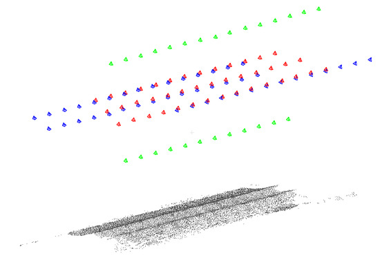
A total of three flights were performed—one single-height nadir-looking flight of 3 strips at 50 m (50-na, na for nadir), one nadir-looking flight of 2 strips with one strip at 30 m and the other at 70 m (3070-na) and one single-height oblique-looking flight of 3 strips at 50 m (50-ob, ob for oblique). See Figure 1b and Table 1 for more detail on the conducted flights. We are interested in these flight configurations since the single-height nadir-looking flight (50-na) is often the routine flight configuration whereas it is not always favourable. The single-height oblique-looking flight 50-ob is, on the contrary, interesting, but is not always easy to conduct. The multi-height nadir-looking flight 3070-na is a possible alternative to 50-ob, since it introduces different flight heights and eases the correlation between parameters on the vertical axes [24].
The acquired images were then processed with MicMac, a free, open-source photogrammetric software which has been developed at IGN since 2003 [25]. Firstly, tie points were extracted on overlapping images with the algorithm SIFT (Scale Invariant Feature Transform) [26]. Then, the structure-from-motion was performed to recover camera poses in an arbitrary frame. The camera model Fraser [8] was chosen to model the camera distortion. The employed Fraser camera model includes the following parameters:
- •
- f: the focal length;
- •
- : the principal point
- •
- : 3 degrees of radial distortion coefficients with the radial distortion being expressed as:
- •
- : tangential distortion coefficients with the tangential distortion being expressed as:
- •
- : affine distortion coefficients with the affine distortion being expressed as:
Next, a total of 14 well-distributed GCPs were used to transform the camera poses into the absolute frame, the image measurement of these GCPs was conducted manually. At last, a bundle block adjustment was performed with the tie points and the GCPs serving as observations. The processing accuracy was evaluated by the root mean square error (RMSE) on control points (CPs) and was 1 cm. More data processing details of the presented dataset are given in Reference [24].
The tie points, the camera calibration and the camera poses issued from the above-presented processing were used to generate a synthetic, error-free dataset. The generation of the synthetic image block was carried out with MicMac. For a set of 2D points representing the same 3D point, a pseudo-intersection was performed to obtain the corresponding 3D coordinates. For a pair of images with two tie points and representing 3D point P, its 3D coordinates were computed, given camera poses and (cf. Figure 3). For a set of 2D points representing a same 3D point P, image pairs are formed and 3D points were computed. Then, the 3D coordinates of the point P were calculated so that the sum of the residual distances was minimized. Afterwards, the 3D point P was reprojected to images for the generation of synthetic tie points. Note that the tie points generated this way intersect perfectly. A subset of the synthetic 3D points uniformly distributed within the scene (around 5000 ground points) also served as GCPs/CPs, their corresponding reprojections on images will serve as image measurements of GCPs/CPs. Figure 4 depicts how the synthetic dataset was generated.
The synthetic dataset consists of synthetic tie points, synthetic GCPs/CPs and their image measurements, original camera calibration and original camera poses. For the synthetic dataset, the reprojection RMSE on images equals 38.4 nm/0.006 pixels and the RMSE on CPs is 3.1 nm, these two indicate a good consistency among observations of the synthetic dataset. It also indicates the highest accuracy one can obtain with this synthetic dataset.
2.2. Problem Simulation and Result Evaluation
According to the research purposes, different camera calibration problems were simulated and added on the synthetic dataset. The photogrammetric processing of the synthetic dataset was performed with MicMac.
A bundle block adjustment was carried out with the synthetic tie points as observations. The camera calibration and the camera poses are given as the initial solution. Depending on the investigation purpose, camera calibration parameters are either fixed or re-estimated during the bundle block adjustment. Specifications will be given for each case. Since the bundle block adjustment was conducted solely with tie points and no ground truth (e.g., GCPs, GNSS) is included, once the bundle block adjustment was done, ten well-distributed GCPs were employed for the determination of a 3D spatial similarity and the camera poses were transformed into the absolute frame of ground points. The accuracy of the 3D scene will be evaluated with the RMSE of 5000 well-distributed CPs.
3. Experiments and Results
In this section, we present three issues with the camera calibration, as well as the conducted experiments and the corresponding results.
3.1. Erroneous Focal Length
The first issue is the erroneous focal length in the case of camera pre-calibration. It is one of the common problems in photogrammetric processing. When the camera is pre-calibrated in a laboratory, the focal length estimated with close-range photogrammetry can be inaccurate in aerial scenarios [15]. To investigate how camera poses and 3D accuracy are affected by the erroneous focal length, an error which varies from −50 pixels to +50 pixels with a step of 10 pixels is added to the original focal length (original value: 5510 pixels).
Three configurations are investigated here: (a) 50-na + 50-ob, (b) 50-na + 3070-na, (c) 50-na + 3070-na + 50-ob. The configuration (a) was a routine acquisition configuration, oblique images were combined with nadir images to achieve better results. The configuration (b) is one configuration that we want to investigate; we want to see whether multi-height nadir images, which are easier to acquire than oblique images, can be an alternative to oblique images. The configuration (c) aims to examine whether multi-height nadir images can further improve the acquisition accuracy achieved with configuration (a).
In the first place, the erroneous camera pre-calibration is given as the initial solution to the bundle block adjustment. During the bundle block adjustment, the focal length, as well as the other camera calibration parameters, was fixed while the camera poses were freed and re-estimated. Figure 5 depicts the resulted accuracy evaluated with the RMSE on CPs and the variation of the camera average height for the 3 configurations.
One can see that the RMSE increases linearly with the error on focal length. The sign of the error does not affect the amplitude of the RMSE. The combination of oblique and nadir images (config (a)) gives the highest RSME, whereas the combination of multi-height nadir images (config (b)) shows better results. On the basis of combining oblique and nadir images, the inclusion of multi-height nadir images (config (c)) improves slightly the accuracy. By analyzing the variation of the average camera height, one can deduce that, when the focal length is erroneous and not re-estimated during the bundle block adjustment, the camera poses drift in the vertical direction to compensate for the impact coming from the erroneous focal length. The presence of oblique images (config (a) and (c)) adds constraints on the camera poses, hence a smaller variation of the average camera height compared to the case where only nadir images are present (config (b)). The inclusion of oblique images results in camera poses closer to the theoretical values, whereas the 3D accuracy is compromised in our cases.
In a second step, the same error is added to the focal length, while the camera calibration parameters are freed and re-estimated during the bundle block adjustment. For all the three configurations, the correct focal length is able to be recovered, the final RMSEs on CPs are smaller than 1 μm. Compared to the RMSE of the original dataset (3.1 nm) and that of the former case (3.5 cm), the camera re-calibration is effective for the correction of the erroneous focal length.
3.2. Gradually Varied Focal Length
In this part, another possibility for false focal length is simulated—the camera focal length varies gradually during the acquisition whereas this variation is not taken into account during the processing. Several studies have been conducted on the influence of the camera temperature on the internal parameters. Hothmer listed various sources of errors in aerial photogrammetric scenarios, among which, the effect of temperature is mentioned [27]. Yastikli and Jacobsen discussed about the vertical temperature gradient and the significant deformation of the camera lens caused by it [28]. Merchant investigated the variation of the focal length induced by the temperature change for a Nikon lens of 20 mm, a variation of 0.5 μm per degree is observed [29,30]. Daakir and Zhou calibrated and corrected the image deformation caused by the variation of camera internal temperature, the 3D reconstruction accuracy was improved by 1.4 times for an aerial dataset of corridor configuration [31].
In UAV photogrammetry, the variation of focal length is often encountered when the acquisition is carried out with a high frame rate. However, during photogrammetric processing, one often assumes that the camera calibration parameters do not vary and one camera calibration is applied to the whole dataset. This processing strategy is sometimes inappropriate and degrades the final accuracy. In this experiment, how the ignorance of the focal length variation impacts different aerial acquisition configurations is studied.
To simulate this problem, starting from the synthetic image block, one camera calibration is estimated per image with the synthetic tie points and the original camera poses. The focal length is modified then so that it varies during the acquisition. Tie points and GCPs/CPs image measurements are regenerated based on original camera poses and modified camera calibrations. After that, the dataset is processed with one camera calibration for all images as which is usually done in the practice. During the bundle block adjustment, no elimination is performed on tie points, all camera calibration parameters are freed and re-estimated.
We generate a linear focal length variation which is expressed by the equation:
where
n is the image index
f is the original focal length;
b is the increment, here b equals to 0.0275 pixels;
f′(n) is the modified focal length for image n;
It is not certain that the focal length increases linearly in real life. Actually, as shown in Reference [31], the increment speed of the temperature decreases with time and the focal length increases linearly with the temperature. Here, the linear model is chosen to model the focal length variation for its simplicity of interpretation. It gives us a first hint of how the final accuracy is impacted when the focal length varies during the acquisition. The focal length of the last image (5513.48 pixels) is 3.10 pixels greater then that of the first image (5510.38 pixels). According to the relation between the focal length and the camera internal temperature given by Reference [31], an increase of 3.10 pixels corresponds to a temperature increase of around 40 °C for a focal length of 35 mm as in our experiments. The amplitude of the temperature variation is realistic and conforms to real acquisition conditions.
To investigate the impact of the flight configuration and the flight order of which the focal length variation takes place, as well to see if there exists one flight configuration that can minimize the influence of varied focal length, different flight combinations and flight orders are exploited. Note that the temperature increment per image is set to 0.0275 pixels as in Equation (1) and is independent of the order in which flights are carried out. The mapping accuracy for each configuration is given in Table 2.
Though the RMSE on CPs may seem small, its order of magnitude is coherent with what is obtained in the previous case of erroneous focal length (Section 3.1). In the previous case, a bias of 10 pixels on focal length causes residuals about 5 mm, when both nadir and oblique images are included. In the presented case of 50vt + 50ob + 3070vt, the focal length has a variation of 3.1 pixels, the estimate of the focal length differs from the real value by 1.5 pixels at most.
Three flight orders are investigated, for each flight order, the number of flights needed to obtain a satisfying accuracy is studied.
1 Flight
If surveying the field with one flight, the oblique-looking flight at 50 m (50-ob) gives better results than the nadir-looking flight (50-na). Similar to the case of erroneous focal length, the presence of oblique images prevents the camera position from drifting to compensate for the incoherence on the focal length, thus leads to better results. When performing the single-height nadir-looking flight (50-na), a slight focal length variation of 1.11 pixels can cause an accuracy degradation of 1 cm.
2 Flights
If two flights are conducted for mapping, the best solution is to perform a nadir-looking flight (50-na) in addition to an oblique one (50-ob). However, when inverting the flight order, though the addition of oblique flight improves significantly the mapping accuracy with respect to one nadir flight, it is less satisfying than performing one oblique flight. It is not recommended to add nadir strips of different flight height (3070-na) to the flight 50-na, since it enlarges the focal length variation and does not limit camera position drift as oblique images.
3 Flights
We see that though same flights are conducted, the order of flight influences the final accuracy. The best order is to perform firstly oblique-looking flights, then nadir ones. By comparing with 2 flights cases, the inclusion of multi-height nadir-looking flights (3070-na) has negative influence when the acquisition suffers from thermal effect. This said, the addition of multi-height nadir-looking flights still brings improvements on other aspects, for instance, it eases the correlation between camera focal length, camera height and lever-arm for mapping of flat scenes [24].
3.3. Error Coming from Rolling Shutter Effect
This section studies the rolling shutter effect and its impact on aerial photogrammetric accuracy. Nowadays, the majority of consumer grade cameras are equipped with rolling shutter. For cameras equipped with a rolling shutter, the image sensor is activated and read out line by line. The exposure of one image takes place between the exposures of the first and the last line, an important delay due to the readout time is present. Figure 6 gives an illustration of the general rolling shutter scheme.
In aerial photogrammetry, the UAV navigates at a high speed (e.g., 2 m/s–10 m/s) and mainstream rolling shutter cameras available on the market for aerial acquisitions have a readout time varying between 30 ms and 80 ms (the readout time for several widely-used cameras are given in https://www.pix4d.com/blog/rolling-shutter-correction). This means the position of the camera can be changed by several centimeters during exposure, the turbulence of UAV adds as well camera orientation changes. This effect is often not taken into account either in the camera calibration or in the photogrammetric processing. Without appropriate modeling, distortions due to rolling shutter limit the accuracy of the photogrammetric reconstruction [32,33,34]. Furthermore, it is also difficult to quantify the deformation in images introduced by the rolling shutter effect, which reduces the possibility of having effective corrections.
To understand better how the rolling shutter effect impacts the final results and by which level, image observations are modified such that each line is acquired with a different camera pose. We assume a uniform camera motion during the exposure. The parameters employed for the generation of simulated camera motion are listed, the value and the justification are given as follows:
- -
- T: time interval between two images, 2.5 s, conforms to real acquisition condition of the presented dataset
- -
- : readout time of rolling shutter camera, 50 ms, a middle value among widely-used rolling shutter cameras
- -
- : camera translational velocity, ∼3 m/s, for each image i, the instantaneous velocity is calculated as the ratio between the displacement and the time interval T of image i and , the value conforms to real acquisition condition of the presented dataset
- -
- : camera rotational velocity, with = 0.02°/s and = 0.016°/s, the rotational axis is generated randomly, the amplitude of rotation angle follows the Gaussian distribution, the value of parameters and comes from IMU data of previous lab acquisitions. The rotational axis is generated here to be random, whereas in practice the axis depends on the type of UAV, the installation and the specification of the motor and the resulted vibration. The assumption of randomness is made, so that a general conclusion can be drawn without being limited to specific conditions.
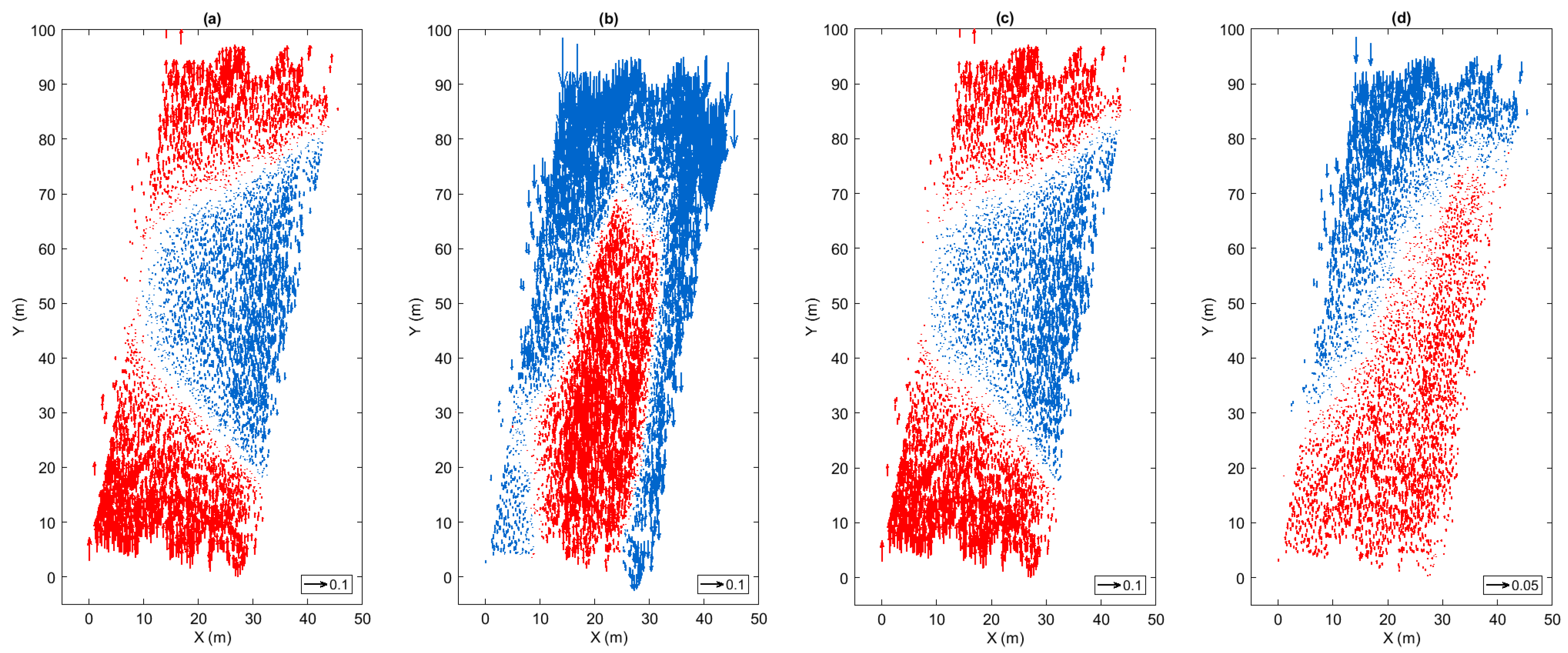
The simulated rolling shutter effect is added to the synthetic dataset by modifying image measurements. After that, the dataset is processed without taking into account camera motion during exposure. Concerning the bundle block adjustment, no elimination is performed on tie points, all camera calibration and pose parameters are freed and re-estimated. In order to simplify the analysis, the camera rotational motion and translational motion are separated. To investigate the impact of flight configuration and to see if there exists one flight configuration that can minimize the rolling shutter effect, four flight configurations are investigated: (a) 50vt, (b) 50vt + 3070vt, (c) 50vt + 50ob, (d) all flights (cf. Figure 7). Figure 8, Figure 9, Figure 10 and Figure 11 illustrate the spatial distribution of residual on CPs for each case and Table 3 gives statistic information.
In Figure 8 and Figure 9, we see that the rotational motion introduces little residuals in planimetry and can be diminished with the inclusion of nadir flights of different heights and oblique images. The altimetric residuals introduced by the rotational motion is slightly higher when there are no oblique images (cases (a) and (b)). Once oblique images are present, the altimetric residuals decrease significantly (cases (c) and (d)). The spatial distribution of residuals changes with flight configuration, we can see a minor bowl effect in all four cases, presenting in different forms.
In Figure 10 and Figure 11, we see that the inclusion of nadir images of different heights degrades largely the accuracy both in planimetry and altimetry. The inclusion of oblique images does not bring significant improvements. The spatial distribution of residuals changes with flight configuration. There is no one flight configuration that is satisfying.
It is worth noting that, the residuals introduced by camera rotational motion can be easily eliminated with the inclusion of more flight strips, such as oblique images and nadir flights of different heights. Compared to the residuals introduced by camera translational motion, the one introduced by rotational motion can be considered negligible. The camera translational motion can largely decrease the accuracy of the obtained results and improvement on flight patterns can not really solve the problem. Therefore, it is essential to perform corrections when processing with rolling shutter datasets.
4. Discussion
For aerial acquisitions of corridor configuration, the acquired images are often in strips, which makes it difficult to have satisfying cross-track overlaps and results in less accurate camera calibration and camera poses. It is a common strategy to perform independently camera pre-calibration in lab prior or post aerial acquisitions. However, the camera pre-calibration performed in a close-range scenario can be inaccurate for aerial scenarios due to different scene depths [15]. The focal length is one of the most impacted parameter in the camera calibration. The experiment carried out with the synthetic, error-free dataset shows that, when combining nadir and oblique images or nadir images of multiple flight heights, the erroneous focal length can be correctly re-estimated during the bundle block adjustment. However, if the camera re-calibration is not performed, the camera poses will drift in the vertical direction to compensate for the incoherence introduced by the erroneous focal length, in order to achieve better 3D measurement accuracy. The presence of oblique images limits this drift, hence results in more accurate camera pose estimations, as shown in References [19,20,21]. In practice, it is recommended to perform camera re-calibration when a good flight geometry is available. Oblique images being critical in forming a good flight geometry, they are more difficult to acquire. In this experiment, we demonstrated the possibility of employing multi-height nadir images as an alternative to oblique images.
In the case where the camera focal length varies gradually during the acquisition, the oblique images show their importance. The best strategy is to perform in the first place an oblique flight, knowing that oblique images limit the camera pose drift caused by the incoherence on the focal length. The addition of nadir images further improves the 3D measurement accuracy while it should be following a certain order. It means the oblique flight should be performed before the nadir flight. For this problem, multi-height nadir images do not bring improvements since it enlarges the focal length variation. However, it is still a good strategy in practice since it brings improvements on other aspects.
The rolling shutter effect is a common problem when performing aerial acquisitions with consumer-grade UAV platforms. With multiple flight configurations (oblique images, multi-height nadir images), the degradation induced by camera rotational motion can be diminished significantly. Mounting the camera on a stabilizer is as well a good practice to minimize the influence of the camera rotational motion. The camera translational motion impacts the final accuracy in a more complicated manner. Certain commercial software offer solutions to correct this impact by estimating the camera motion during the bundle block adjustment [32,35]. Among the flight configurations investigated in our experiment, none of them gives satisfying results. In practice, performing the acquisition in “stop-and-go” mode may be an easier way to obviate the impact of the rolling shutter effect. The improvement of “stop-and-go” mode requires further investigations.
In a nutshell, it is always beneficial to diversify the flight geometry. The oblique images should be considered as the first solution as it is an effective approach in many aspects. If possible, it is also recommended to include multi-height nadir images or make it an alternative to oblique images.
5. Conclusions
In this article, we studied the impact of different camera calibration issues with a synthetic aerial image block of flat, corridor configuration. The synthetic, error-free aerial image block gives the possibility to investigate the problematic of interest without the perturbation of other sources.
For a camera calibration given as initial solution, the error on focal length can be corrected during the bundle block adjustment with a good acquisition configuration. However, when an erroneous focal length is given and not re-estimated during the bundle block adjustment, camera heights drift from theoretical values to compensate for the erroneous focal length. The presence of oblique images limits this drift, therefore camera poses closer to theoretical values are obtained whereas the accuracy of 3D measurement is compromised.
Secondly, the focal length is likely to vary during acquisitions due to the temperature change of the camera. When this variation is not taken into consideration and one camera calibration is given for the whole dataset, an important degradation of accuracy can occur, mainly in altimetry. When only nadir images are present, a variation of 1 pixel of the focal length can decrease the 3D accuracy by 1 cm. The inclusion of oblique images brings a significant improvement, which is a good solution to the problem. It is even more recommended to perform oblique flight before nadir ones. The single-strip nadir-looking flights (3070vt) does not have visible improvements on the problem.
As for the degradation of rolling shutter effect, the degradation introduced by camera rotational motion can be easily eliminated with the inclusion of more flight strips. However, this improvement is negligible compared to the degradation brought by camera translational motion. There is no flight configurations that really work out, the more efficient solution should be a correction on image measurements that are affected by the rolling shutter effect.
In this article, two cases regarding the focal length estimation are discussed (the erroneous focal length and the gradually varied focal length). It is one of the important parameters of the camera distortion. It is also worth investigating other parameters such as the radial distortion parameter and how they impact the doming effect and the final accuracy. The gradually varied focal length subject to camera temperature change is modelled with a linear model for simplicity of interpretation. For future works, models better illustrating the real case conditions should be applied. The last experiment showed that the influence of the camera rotational motion is negligible with respect to the camera translational motion. This is one result that can be taken into account when implementing rolling shutter correction methods.
Author Contributions
Y.Z. and M.P.-D. provided the initial idea for this study; Y.Z. conceived and designed the experiments; Y.Z., C.M. and C.T. analyzed the data; Y.Z. wrote the main manuscript; and E.R. reviewed the manuscript. All authors have read and agreed to the published version of the manuscript.
Funding
This research is funded within the Ph.D thesis of Y.Z.
Conflicts of Interest
The authors declare no conflict of interest.
References
- Nex, F.; Remondino, F. UAV for 3D mapping applications: A review. Appl. Geomat. 2014, 6, 1–15. [Google Scholar] [CrossRef]
- Heipke, C.; Jacobsen, K.; Wegmann, H. Analysis of the results of the OEEPE test “Integrated Sensor Orientation. In OEEPE Integrated Sensor Orientation Test Report and Workshop Proceedings, Editors; Citeseer: Hannover, Germany, 2002. [Google Scholar]
- Cramer, M.; Stallmann, D.; Haala, N. Direct georeferencing using GPS/inertial exterior orientations for photogrammetric applications. Int. Arch. Photogramm. Remote Sens. 2000, 33, 198–205. [Google Scholar]
- Westoby, M.; Brasington, J.; Glasser, N.; Hambrey, M.; Reynolds, J. ‘Structure-from-Motion’ photogrammetry: A low-cost, effective tool for geoscience applications. Geomorphology 2012, 179, 300–314. [Google Scholar] [CrossRef] [Green Version]
- Fonstad, M.A.; Dietrich, J.T.; Courville, B.C.; Jensen, J.L.; Carbonneau, P.E. Topographic structure from motion: A new development in photogrammetric measurement. Earth Surf. Process. Landf. 2013, 38, 421–430. [Google Scholar] [CrossRef] [Green Version]
- Duane, C.B. Close-range camera calibration. Photogramm. Eng. 1971, 37, 855–866. [Google Scholar]
- Schut, G. Selection of additional parameters for the bundle adjustment. Photogramm. Eng. Remote Sens. 1979, 45, 1243–1252. [Google Scholar]
- Fraser, C.S. Digital camera self-calibration. ISPRS J. Photogramm. Remote Sens. 1997, 52, 149–159. [Google Scholar] [CrossRef]
- Ebner, H. Self calibrating block adjustment. Bildmessung Luftbildwessen 1976, 44, 128–139. [Google Scholar]
- Gruen, A. Accuracy, reliability and statistics in close-range photogrammetry. In Proceedings of the Inter-Congress Symposium of ISP Commission V, Stockholm, Sweden, 14–17 August 1978. [Google Scholar]
- Fraser, C.S. Automatic camera calibration in close range photogrammetry. Photogramm. Eng. Remote Sens. 2013, 79, 381–388. [Google Scholar] [CrossRef] [Green Version]
- Remondino, F.; Fraser, C. Digital camera calibration methods: Considerations and comparisons. Int. Arch. Photogramm. Remote Sens. Spat. Inf. Sci. 2006, 36, 266–272. [Google Scholar]
- James, M.R.; Quinton, J.N. Ultra-rapid topographic surveying for complex environments: The hand-held mobile laser scanner (HMLS). Earth Surf. Process. Landf. 2014, 39, 138–142. [Google Scholar] [CrossRef] [Green Version]
- Harwin, S.; Lucieer, A. Assessing the accuracy of georeferenced point clouds produced via multi-view stereopsis from unmanned aerial vehicle (UAV) imagery. Remote Sens. 2012, 4, 1573–1599. [Google Scholar] [CrossRef] [Green Version]
- Lichti, D.; Skaloud, J.; Schaer, P. On the calibration strategy of medium format cameras for direct georeferencing. In Proceedings of the International Calibration and Orientation Workshop EuroCOW, Castelldefels, Spain, 30 January–1 February 2008. [Google Scholar]
- Rosnell, T.; Honkavaara, E. Point cloud generation from aerial image data acquired by a quadrocopter type micro unmanned aerial vehicle and a digital still camera. Sensors 2012, 12, 453–480. [Google Scholar] [CrossRef] [PubMed] [Green Version]
- James, M.R.; Robson, S. Mitigating systematic error in topographic models derived from UAV and ground-based image networks. Earth Surf. Process. Landf. 2014, 39, 1413–1420. [Google Scholar] [CrossRef] [Green Version]
- Javernick, L.; Brasington, J.; Caruso, B. Modeling the topography of shallow braided rivers using Structure-from-Motion photogrammetry. Geomorphology 2014, 213, 166–182. [Google Scholar] [CrossRef]
- Castillo, C.; Pérez, R.; James, M.R.; Quinton, J.; Taguas, E.V.; Gómez, J.A. Comparing the accuracy of several field methods for measuring gully erosion. Soil Sci. Soc. Am. J. 2012, 76, 1319–1332. [Google Scholar] [CrossRef] [Green Version]
- James, M.R.; Robson, S. Straightforward reconstruction of 3D surfaces and topography with a camera: Accuracy and geoscience application. J. Geophys. Res. Earth Surf. 2012, 117. [Google Scholar] [CrossRef] [Green Version]
- James, M.; Varley, N. Identification of structural controls in an active lava dome with high resolution DEMs: Volcán de Colima, Mexico. Geophys. Res. Lett. 2012, 39. [Google Scholar] [CrossRef] [Green Version]
- Wackrow, R.; Chandler, J.H. Minimising systematic error surfaces in digital elevation models using oblique convergent imagery. Photogramm. Rec. 2011, 26, 16–31. [Google Scholar] [CrossRef] [Green Version]
- Martin, O.; Meynard, C.; Pierrot Deseilligny, M.; Souchon, J.P.; Thom, C. Réalisation d’une caméra photogrammétrique ultralégère et de haute résolution. In Proceedings of the Colloque Drones Et Moyens Légers Aéroportés D’observation, Montpellier, France, 24–26 June 2014; pp. 24–26. [Google Scholar]
- Zhou, Y.; Rupnik, E.; Faure, P.H.; Pierrot-Deseilligny, M. GNSS-Assisted Integrated Sensor Orientation with Sensor Pre-Calibration for Accurate Corridor Mapping. Sensors 2018, 18, 2783. [Google Scholar] [CrossRef] [Green Version]
- Rupnik, E.; Daakir, M.; Deseilligny, M.P. MicMac—A free, open-source solution for photogrammetry. Open Geospat. Data Softw. Stand. 2017, 2, 14. [Google Scholar] [CrossRef]
- Lowe, D.G. Object recognition from local scale-invariant features. In Proceedings of the Seventh IEEE International Conference on Computer Vision, Kerkyra, Greece, 20–27 September 1999; Volume 99, pp. 1150–1157. [Google Scholar]
- Hothmer, J. Possibilities and limitations for elimination of distortion in aerial photographs. Photogramm. Rec. 1958, 2, 426–445. [Google Scholar] [CrossRef]
- Yastikli, N.; Jacobsen, K. Influence of system calibration on direct sensor orientation. Photogramm. Eng. Remote Sens. 2005, 71, 629–633. [Google Scholar] [CrossRef] [Green Version]
- Merchant, D.C. Influence of temperature on focal length for the airborne camera. In Proceedings of the MAPPS/ASPRS Fall Conference, San Antonio, TX, USA, 6–10 November 2006. [Google Scholar]
- Merchant, D.C. Aerial Camera Metric Calibration—History and Status. In Proceedings of the ASPRS 2012 Annual Conference, Sacramento, CA, USA, 19–23 March 2012; pp. 19–23. [Google Scholar]
- Daakir, M.; Zhou, Y.; Pierrot-Deseilligny, M.; Thom, C.; Martin, O.; Rupnik, E. Improvement of photogrammetric accuracy by modeling and correcting the thermal effect on camera calibration. ISPRS J. Photogramm. Remote Sens. 2019, 148, 142–155. [Google Scholar] [CrossRef] [Green Version]
- Vautherin, J.; Rutishauser, S.; Schneider-Zapp, K.; Choi, H.F.; Chovancova, V.; Glass, A.; Strecha, C. Photogrammetric accuracy and modeling of rolling shutter cameras. ISPRS Ann. Photogramm. Remote Sens. Spat. Inf. Sci. 2016, 3, 139–146. [Google Scholar] [CrossRef]
- Meingast, M.; Geyer, C.; Sastry, S. Geometric models of rolling-shutter cameras. arXiv 2005, arXiv:cs/0503076. [Google Scholar]
- Chun, J.B.; Jung, H.; Kyung, C.M. Suppressing rolling-shutter distortion of CMOS image sensors by motion vector detection. IEEE Trans. Consum. Electron. 2008, 54, 1479–1487. [Google Scholar] [CrossRef]
- Saurer, O.; Pollefeys, M.; Hee Lee, G. Sparse to dense 3D reconstruction from rolling shutter images. In Proceedings of the IEEE Conference on Computer Vision and Pattern Recognition, Las Vegas, NV, USA, 27–30 June 2016; pp. 3337–3345. [Google Scholar]
Figure 1.
Illustration of the acquisition field (a) and the conducted flights (b): nadir flight of 3 strips at 50 m (in red), oblique flight of 3 strips at 50 m (in blue) and nadir flights of 2 strip at 30/70 m (in green).
Figure 1.
Illustration of the acquisition field (a) and the conducted flights (b): nadir flight of 3 strips at 50 m (in red), oblique flight of 3 strips at 50 m (in blue) and nadir flights of 2 strip at 30/70 m (in green).
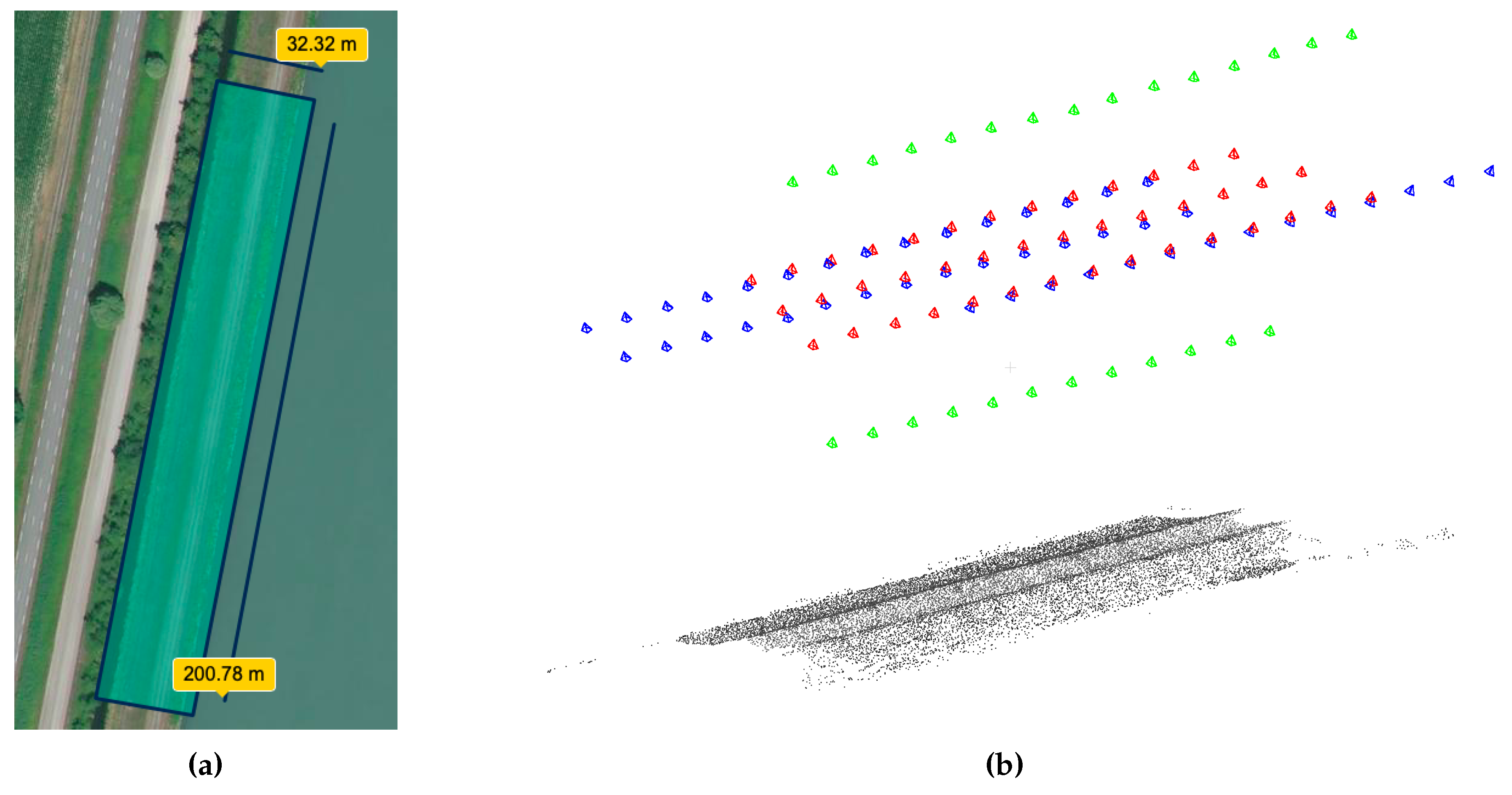
Figure 2.
(a) Light-weight camera; (b) camera set-up on unmanned aerial vehicle (UAV); (c) UAV.
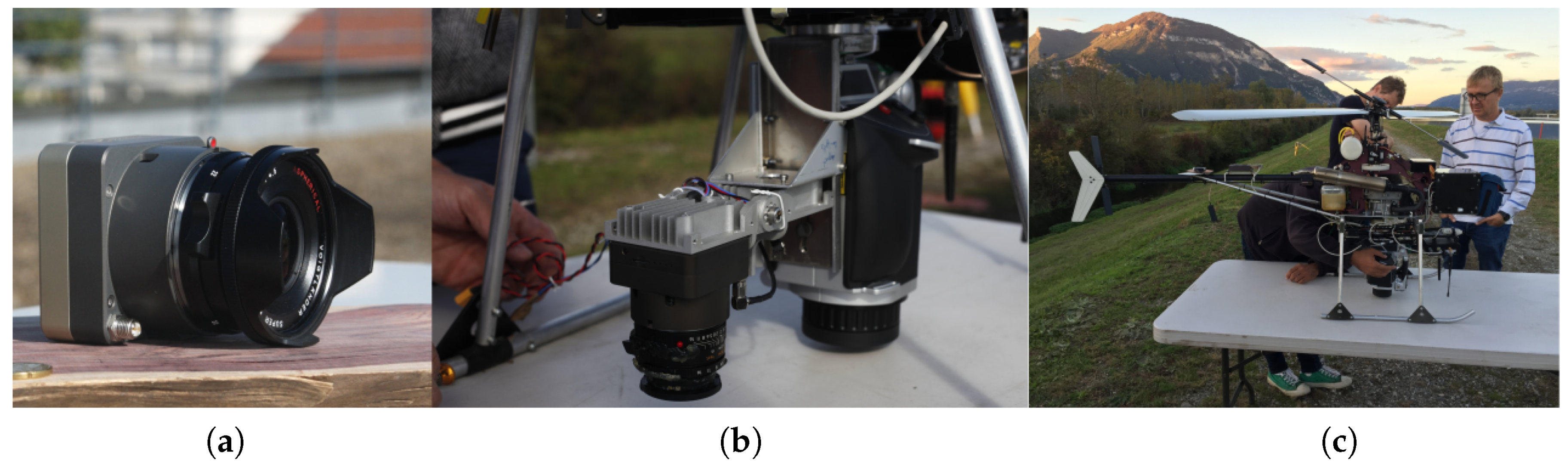
Figure 3.
An illustration of an image pair.
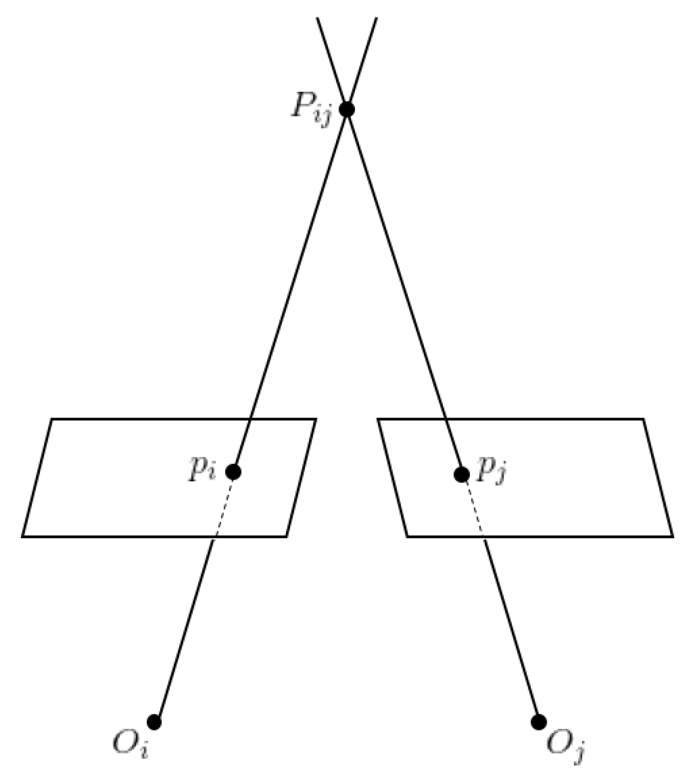
Figure 4.
Workflow of the generation of synthetic dataset.

Figure 5.
The RMSE on control points (CPs) and the variation of the camera height, in the case of erroneous focal length. (a)–(c): the RMSE on CPs for the three configurations, respectively. (d): the variation of the average camera height with error on focal length.
Figure 5.
The RMSE on control points (CPs) and the variation of the camera height, in the case of erroneous focal length. (a)–(c): the RMSE on CPs for the three configurations, respectively. (d): the variation of the average camera height with error on focal length.

Figure 6.
Rolling shutter readout scheme. The sensor is exposed row by row at a constant speed. After the exposure duration , the sensor starts the readout row by row. At time t = 0 the exposure of the first row takes place. It is then read out at time . Consecutive rows are exposed and read out one after the other. The sensor readout is finished after the rolling shutter readout time . (Source: Reference [32]).
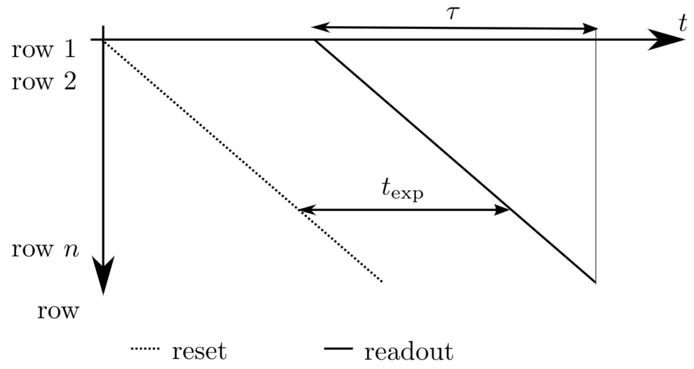
Figure 7.
Four flight configurations: (a) 50vt (b) 50vt + 3070vt (c) 50vt + 50ob (d) all flights. The arrows indicate the flight direction, the colors differentiate the flights.
Figure 7.
Four flight configurations: (a) 50vt (b) 50vt + 3070vt (c) 50vt + 50ob (d) all flights. The arrows indicate the flight direction, the colors differentiate the flights.
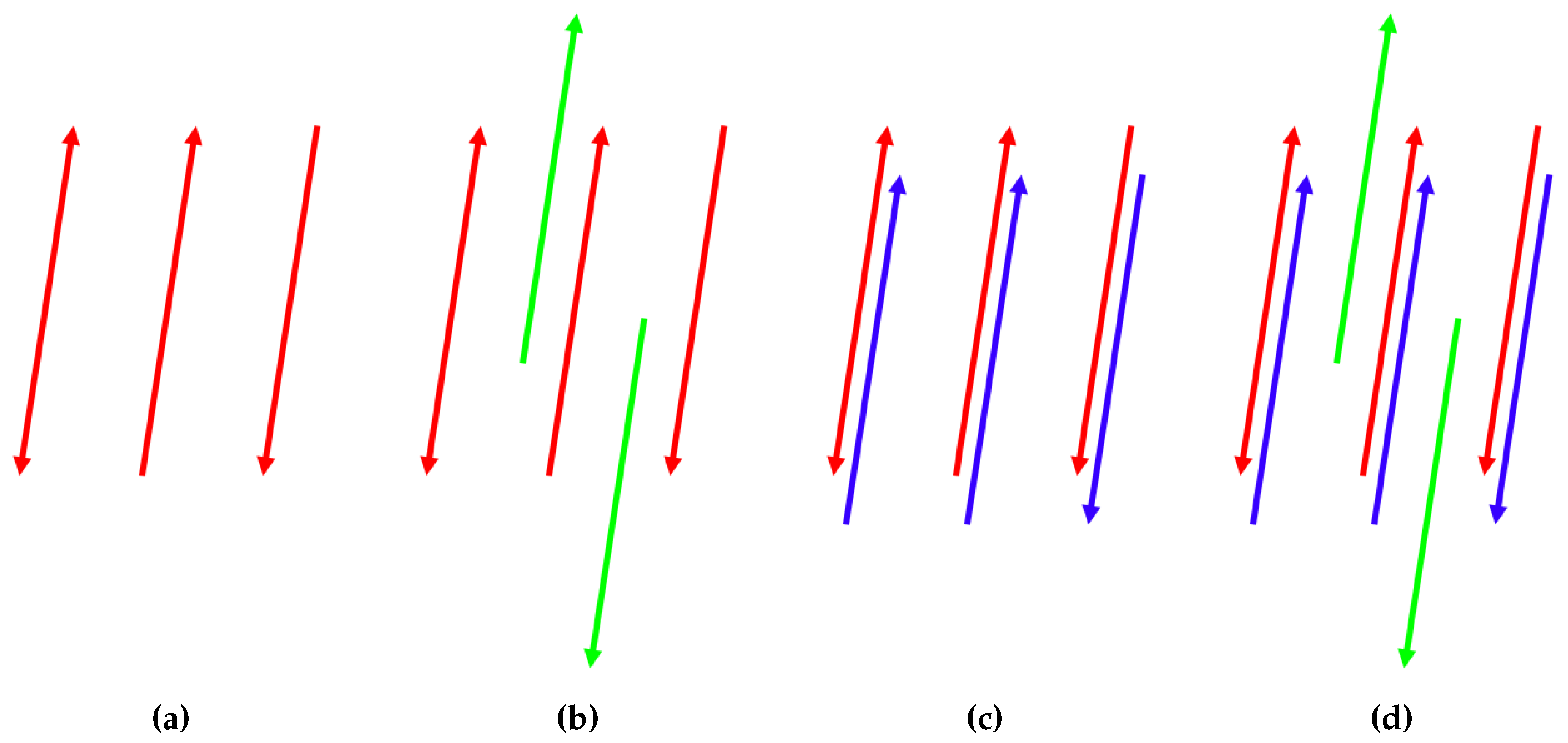
Figure 8.
The spatial distribution of planimetric residuals when the camera rotational motion is added. The presented four cases correspond to the four flight configurations shown in Figure 7. Vector direction and magnitude represent residual direction and magnitude, respectively.
Figure 8.
The spatial distribution of planimetric residuals when the camera rotational motion is added. The presented four cases correspond to the four flight configurations shown in Figure 7. Vector direction and magnitude represent residual direction and magnitude, respectively.
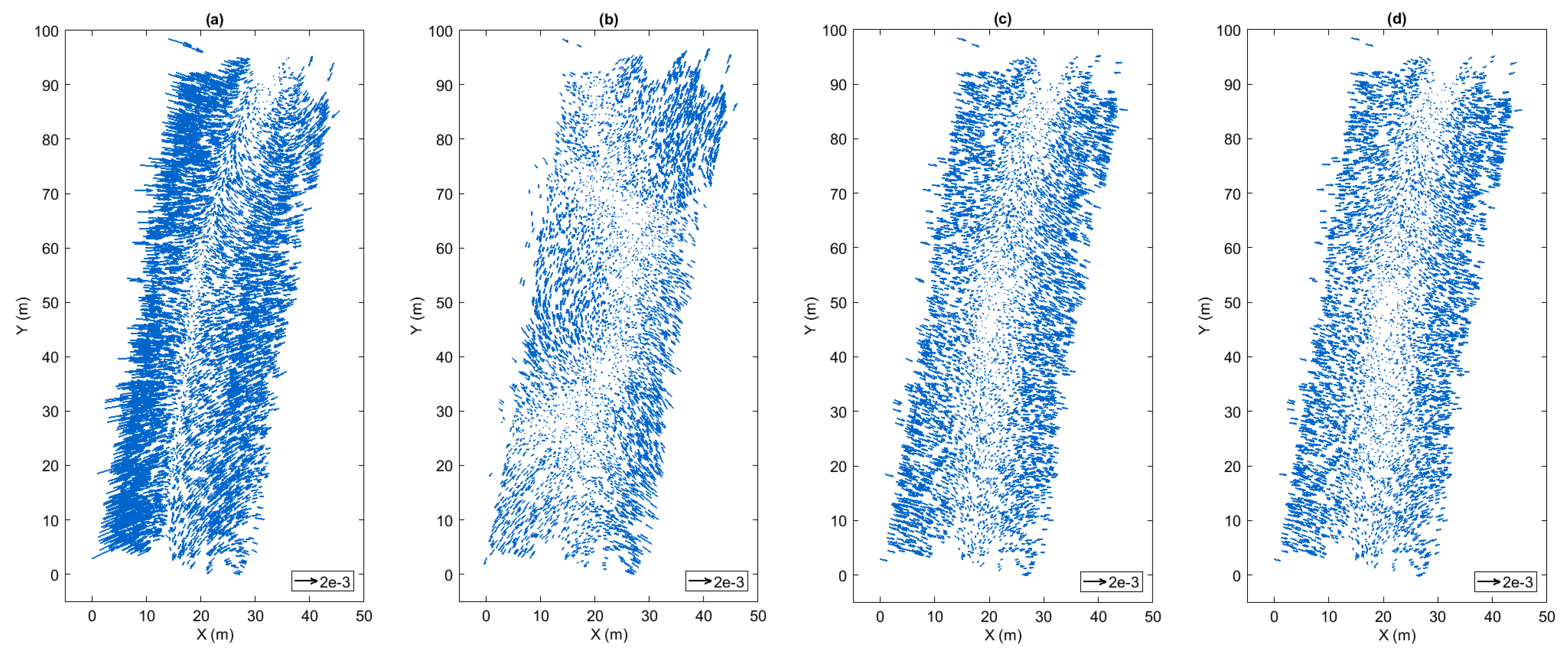
Figure 9.
The spatial distribution of altimetric residuals when the camera rotational motion is added. The presented four cases correspond to the four flight configurations shown in Figure 7. Vector direction and color represent the sign of residuals, upward red means positive, downward blue means negative; vector magnitude represents residual magnitude. Note that the four figures do not share the same scale.

Figure 10.
The spatial distribution of planimetric residuals when the camera translational motion is added. The presented four cases correspond to the four flight configurations shown in Figure 7. Vector direction and magnitude represent residual direction and magnitude, respectively. Note that the last figure does not share the same scale with the other ones.
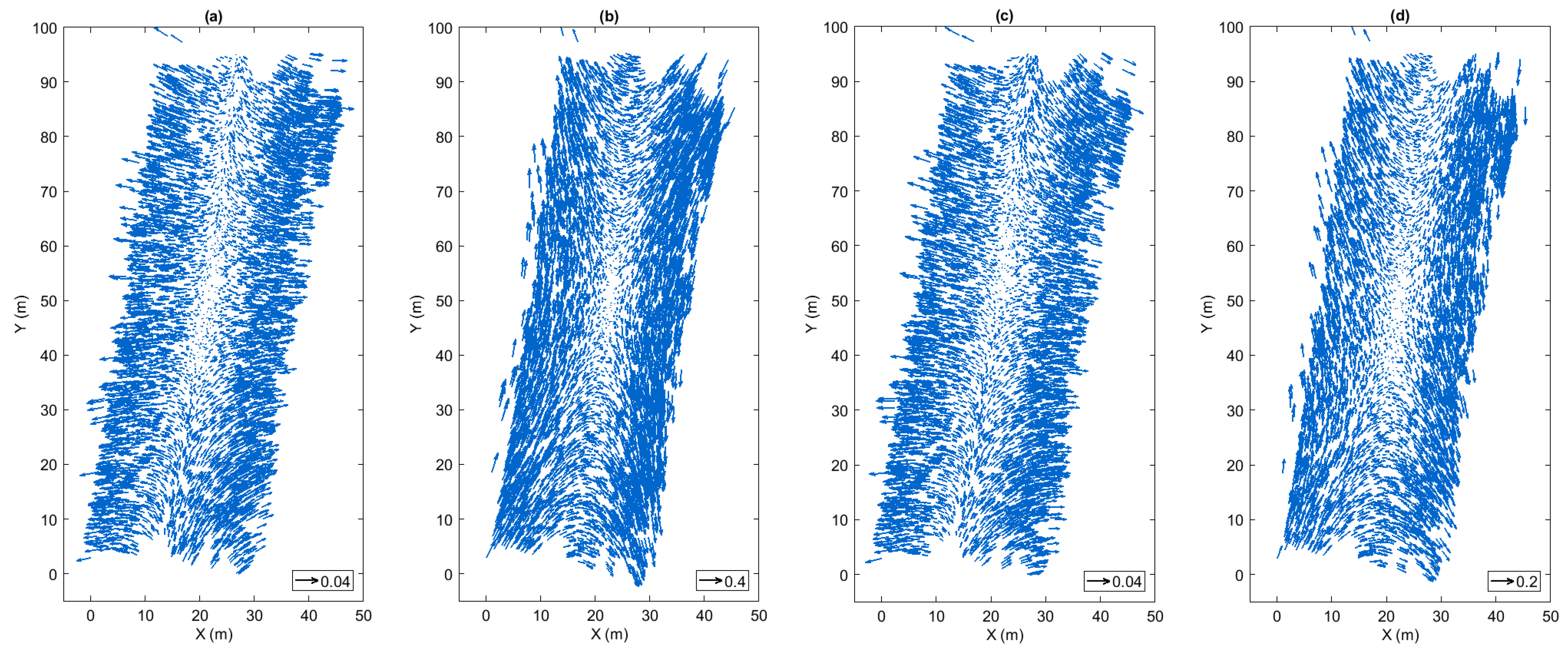
Figure 11.
The spatial distribution of altimetric residuals when the camera translational motion is added. The presented four cases correspond to the four flight configurations shown in Figure 7. Vector direction and color represent the sign of residuals, upward red means positive, downward blue means negative; vector magnitude represents residual magnitude. Note that the four figures do not share the same scale.

Table 1.
Details on the conducted flights.
| Flight | 50-na | 3070-na | 50-ob | |
|---|---|---|---|---|
| Nb of images | 42 | 27 | 44 | |
| Height (m) | 50 | 30, 70 | 50 | |
| Orientation | nadir | nadir | oblique | |
| Nb of strips | 3 | 2 | 3 | |
| Overlap (%) | forward | 80 | ||
| side | 70 | |||
| GCP accuracy (mm) | horizontal | 1.3 | ||
| vertical | 1 | |||
| camera focal length (mm) | 35 | |||
| GSD (mm) | 10 | 6, 14 | 10 | |
Table 2.
Mapping accuracy with different flight configurations and flight orders.
| Focal Length Variation (pixel) | Order 1 | Order 2 | Order 3 | |||||||||||||||||
|---|---|---|---|---|---|---|---|---|---|---|---|---|---|---|---|---|---|---|---|---|
| 50-na, 50-ob, 3070-na | 50-ob, 50-na, 3070-na | 50-na, 3070-na, 50-ob | ||||||||||||||||||
| RMSE (cm) | STD (cm) | RMSE (cm) | STD (cm) | RMSE (cm) | STD (cm) | |||||||||||||||
| xy | z | xyz | xy | z | xyz | xy | z | xyz | xy | z | xyz | xy | z | xyz | xy | z | xyz | |||
| 1 flight | 50-na | 1.11 | 0.02 | 1.01 | 1.01 | 0.01 | 0.13 | 0.13 | / | / | / | / | / | / | / | / | / | / | / | / |
| 50-ob | 1.21 | / | / | / | / | / | / | 0.05 | 0.05 | 0.07 | 0.02 | 0.04 | 0.03 | / | / | / | / | / | / | |
| 2 flights | 50-na+50-ob | 2.36 | 0.02 | 0.09 | 0.09 | 0.01 | 0.04 | 0.04 | 0.01 | 0.01 | 0.02 | 0.01 | 0.01 | 0.01 | / | / | / | / | / | / |
| 50-na+3070-na | 1.89 | / | / | / | / | / | / | / | / | / | / | / | / | 0.05 | 1.08 | 1.08 | 0.00 | 0.14 | 0.14 | |
| 3 flights | 50-na+50-ob+3070-na | 3.10 | 0.02 | 0.11 | 0.11 | 0.00 | 0.06 | 0.06 | 0.01 | 0.03 | 0.04 | 0.00 | 0.03 | 0.02 | 0.03 | 0.17 | 0.17 | 0.01 | 0.05 | 0.05 |
Table 3.
Statistics of the residuals on CPs, the root mean square (RMS) and the unbiased standard deviation (STD) are given.
Table 3.
Statistics of the residuals on CPs, the root mean square (RMS) and the unbiased standard deviation (STD) are given.
| Planimetry (cm) | Altimetry (cm) | 3D (cm) | |
|---|---|---|---|
| Rotation, case (a) | 0.07 ± 0.03 | 0.19 ± 0.19 | 0.20 ± 0.12 |
| Rotation, case (b) | 0.02 ± 0.01 | 0.09 ± 0.08 | 0.09 ± 0.05 |
| Rotation, case (c) | 0.03 ± 0.01 | 0.01 ± 0.01 | 0.03 ± 0.01 |
| Rotation, case (d) | 0.02 ± 0.01 | 0.01 ± 0.01 | 0.03 ± 0.01 |
| Translation, case (a) | 1.44 ± 0.62 | 2.61 ± 2.50 | 2.98 ± 1.51 |
| Translation, case (b) | 18.23 ± 7.93 | 5.36 ± 5.14 | 19.00 ± 7.88 |
| Translation, case (c) | 1.44 ± 0.61 | 2.52 ± 2.43 | 2.90 ± 1.46 |
| Translation, case (d) | 6.88 ± 2.97 | 0.71 ± 0.77 | 6.93 ± 2.97 |
© 2019 by the authors. Licensee MDPI, Basel, Switzerland. This article is an open access article distributed under the terms and conditions of the Creative Commons Attribution (CC BY) license (http://creativecommons.org/licenses/by/4.0/).
Share and Cite
MDPI and ACS Style
Zhou, Y.; Rupnik, E.; Meynard, C.; Thom, C.; Pierrot-Deseilligny, M. Simulation and Analysis of Photogrammetric UAV Image Blocks—Influence of Camera Calibration Error. Remote Sens. 2020, 12, 22. https://doi.org/10.3390/rs12010022
AMA Style
Zhou Y, Rupnik E, Meynard C, Thom C, Pierrot-Deseilligny M. Simulation and Analysis of Photogrammetric UAV Image Blocks—Influence of Camera Calibration Error. Remote Sensing. 2020; 12(1):22. https://doi.org/10.3390/rs12010022
Chicago/Turabian StyleZhou, Yilin, Ewelina Rupnik, Christophe Meynard, Christian Thom, and Marc Pierrot-Deseilligny. 2020. "Simulation and Analysis of Photogrammetric UAV Image Blocks—Influence of Camera Calibration Error" Remote Sensing 12, no. 1: 22. https://doi.org/10.3390/rs12010022
Note that from the first issue of 2016, this journal uses article numbers instead of page numbers. See further details here.