Spatiotemporal Distribution of Human–Elephant Conflict in Eastern Thailand: A Model-Based Assessment Using News Reports and Remotely Sensed Data


Institute of Industrial Science, The University of Tokyo, 4-6-1 Komaba, Meguro-ku, Tokyo 153-8505, Japan
*
Author to whom correspondence should be addressed.
Remote Sens. 2020, 12(1), 90; https://doi.org/10.3390/rs12010090
Submission received: 18 November 2019
/
Revised: 17 December 2019
/
Accepted: 23 December 2019
/
Published: 25 December 2019
(This article belongs to the Special Issue Remote Sensing for Monitoring Wildlife and Habitat in a Changing World)
Abstract
:In Thailand, crop depredation by wild elephants intensified, impacting the quality of life of local communities and long-term conservation of wild elephant populations. Yet, fewer studies explore the landscape-scale spatiotemporal distribution of human–elephant conflict (HEC). In this study, we modeled the potential HEC distribution in ten provinces adjacent to protected areas in Eastern Thailand from 2009 to 2018. We applied the time-calibrated maximum entropy method and modeled the relative probability of HEC in varying scenarios of resource suitability and direct human pressure in wet and dry seasons. The environmental dynamic over the 10-year period was represented by remotely sensed vegetation, meteorological drought, topographical, and human-pressure data. Results were categorized in HEC zones using the proposed two-dimensional conflict matrix. Logistic regression was applied to determine the relevant contribution of each scenario. The results showed that although HEC probability varied across seasons, overall HEC-prone areas expanded in all provinces from 2009 to 2018. The largest HEC areas were estimated during dry seasons with Chantaburi, Chonburi, Nakhon Ratchasima, and Rayong provinces being the HEC hotspots.However, the HEC potential was reduced during severe and prolonged droughts caused by El Nino events. Direct human pressure caused a more gradual increase of HEC probability around protected areas. On the other hand, resource suitability showed large variation across seasons. We recommend zone-dependent management actions towards a fine-balance between human development and the conservation of wild elephants.

1. Introduction
Although wild Asian elephants (Elephas maximus) are listed as endangered species under the IUCN (International Union for the Conservation of Nature) Red List of Threatened Species, their conservation is hampered by humans as a reaction to crop depredation caused by elephants [1]. In Asia, approx. 10%–15% of total agricultural output can be damaged by wild elephants, which threaten human security and well-being [2]. India hosts the largest population of wild Asian elephants: each year, 400 people and 100 elephants die as a result of human–elephant conflict (HEC) [3]. Understanding the HEC phenomenon is critical to both conservation success and the livelihood of human communities in close proximity to wild elephant habitats.
Thailand is estimated to have 3000–3500 wild elephants in 68 areas, 41 of which are facing HEC, commonly in the form of crop depredation [4]. Historically, elephants have been recorded inside Bangkok, Thailand’s capital city, and the surrounding provinces [5]. Nowadays, the estimated home range of wild elephants in the country lies in heavily fragmented landscapes and is surrounded by human-dominated activities [6]. Consequently, interaction between wild elephants and humans became more frequent, increasing the likelihood of conflict.
Across countries with presence of wild elephants, various mitigation strategies have been implemented that include guarding (e.g., watchtowers), deterrents (e.g., firecrackers), physical barriers (e.g., trenches and various form of fences: electric, chilies), translocation of elephants or humans, and compensation [7]. In Thailand, guarding, together with traditional deterrents, are the most common strategies [8]. In high conflict areas, large fences and trenches were constructed by the government, but proved ineffective due to lack of proper maintenance [9]. Recently, more active approaches were employed, such as (i) GPS collaring of wild elephants known to forage outside protected areas to track their movement [10], and (ii) issuing of government insurance schemes for crop damage by elephants [11]. Landscape planning is viewed as a potential long-term solution [12], but its implementation has not yet been established despite being mentioned in the draft of 20-year Master Plan for Elephant Conservation [11].
Apart from the negative human–elephant interaction, HEC also includes conflicting human objectives [13,14]. Social factors, such as trust in authority, education, income, culture, and religion, influence community tolerance and willingness to coexist with elephants [12,15]. Simultaneously, competition for scarce resources between humans and wildlife in a shared landscape remains a fundamental cause of conflict [16,17]. Knowledge of the spatiotemporal variation of resources and its effect on the pattern of conflict is an important initial step toward a sustainable, long-term solution [18].
Studies in Thailand generally focus on social aspects of HEC, such as people’s attitudes and perceptions [19,20], conservation, and legal management [21,22]. An existing study on the spatial distribution of wild elephants included only localized habitat suitability assessment in a single conservation area [5]. Studies on spatiotemporal patterns of HEC across landscapes remain limited but they are crucial for appropriate decision making [23]. Compared to African elephants, such studies are relatively few in Asia [18,24,25] and, to the best of our knowledge, no such study exits in Thailand.
Species Distribution Models (SDMs) are widely used in ecology to predict spatial patterns of species. SDMs are numerical models that quantify the relationship between ecological (e.g., species/population abundance) and environment variables [26]. SDMs estimate the environmental similarity between locations to known ecological response and extrapolates from local samples to entire target landscapes. Their application has been seen in human-wildlife conflicts [27], but remains relatively few in HEC modeling.
Previous ecological studies on elephants have researched the seasonal variation in elephant movement and dispersal [28,29]. Nevertheless, SDMs commonly employ environmental data that provide less dynamic information with often irrelevant temporal resolution between predictor and response variables. This is specifically true for meteorological time series, which are often interpolated from weather stations, introducing uncertainty due to uneven data distribution and availability in developing countries [30]. In contrast, remotely sensed satellite datasets can provide spatially explicit and continuous observation which are believed to enhance SDM accuracy [31]. Previous studies highlighted model-performance improvement due to the utilization of remote sensing datasets, such as vegetation phenology [32], and human activities [33]. In addition, a generic assumption in SDMs is that ecological response can be described by a single function, which results in over-simplification [34], reducing the ability to identify drivers of response [35]. Specifically in habitat modeling, a single function SDM will overlook certain management areas (e.g., sink-like habitat) when key factors that determine the occurrences are not positively correlated [36]. Therefore, modeling occurrences based on two SDMs from the perspective of different key factors allows for a more informative assessment [35,36,37]. HEC, in particular, depends on two prominent physical variables: resource suitability and human pressure. Such a two-dimensional approach has not yet been applied in HEC modeling.
The aim of this study was to bridge the knowledge gap on the physical factors that potentially govern the spatial distribution of HEC in Eastern Thailand. Given the large landscape extent and the dynamic spatiotemporal variation of environmental and physical factors, we utilized remotely sensed satellite data and quantified the spatiotemporal HEC distribution over a 10-year period. Our specific objectives were to (i) model the potential spatial distribution of seasonal HEC from 2009 to 2018 with the use of time-calibrated SDMs, (ii) identify and distinguish the contribution over time of important modeling factors (resource suitability and direct human disturbance), and (iii) prioritize the areas that require targeted management and increased intervention.
2. Materials and Methods
2.1. Study Area
Our study was carried out in two forest-dominated areas of Eastern Thailand (Figure 1) covering eight eastern and two north-eastern provinces. The area has a tropical monsoon climate. The monsoon season occurs from mid-May to mid-October with an average rainfall of 1400 mm, while the area during dry season receives about 400 mm of rainfall [38,39]. The region has nine national parks (NP) and wildlife sanctuaries (WS) hosting elephants [5]. Khao Angruenai-WS, for example, experiences high density of wild elephants, approx. 0.2 elephant/km [40]. In addition, a constantly low elevation in the central region enabled elephants to easily disperse into agricultural land. Consequently, this area is suspected to be a HEC hotspot. Agriculture is the dominant land cover. The five most important crops in planting areas are rice, cassava, rubber plant, sugarcane, and maize. Orchards and plantations commonly spread out in the southern areas. To limit the modeling boundary to only those potentially accessible by elephants, a 20-km buffer was created from the boundary of protected areas and village location with reported HEC. The seasonal models were set according to the monsoon pattern, with May to October as the wet season and November to April of the following year as the dry season.
2.2. Data
HEC occurrences were collected from online news reported between 2014 to 2018. The environmental predictors were prepared under the same time period. Based on this data, we modeled the spatial distribution of HEC across the study area for the period 2009–2018 and developed maps of HEC category. The flow chart of this study is shown in Figure 2.
2.2.1. HEC Occurrence Data
Until March 2019 when elephant-induced damages were first included in farmers’ insurance schemes, HEC was neither compensated, nor insured by the Thai government [11]. Consequently, official records were not consistently maintained across protected areas. Although elephants’ locations outside of protected areas were sometimes documented, the presence of elephants is not always equivalent to HEC. Reporting from news sources usually happens when negative outcomes occur, and this better reflects HEC occurrences. Therefore, HEC incidences were retrieved from online news sources. ‘Wild elephants’ in Thai language was used as a search keyword from the News section of Google Search Engine. A customized time period was set between 2014 and 2018. Each search output was investigated manually to exclude duplicated reports of the same incident.
The news reports, however, did not mention the precise locations of HEC occurrence but only the village names. To overcome this lack of exact occurrence locations, we simulated the occurrence locations using a conditional random sampling method. The sampling boundaries were restricted within a 3-km buffer around the center of each mentioned village, excluding areas that fall within the protected areas, large water bodies (e.g., reservoirs), and major road networks. We excluded locations with the aforementioned features because HECs are unlikely to occur within them. The numbers of random occurrence points were generated according to the numbers of damage incidents reported within each village. A total of 124 incidents occurred in the wet season; a combination of 7, 12, 14, 31, and 60 incidents from 2014 to 2018 respectively. The dry season had 122 reports in total; 5, 20, 20, 20, and 57 of which occurred respectively in the same period of time.
Five sets of random occurrences were generated. A Wilcoxon–Mann–Whitney test [41] was performed to compare the distribution profile of each independent variable to that of the other four sets of simulated occurrence records. A p-value of over 0.05 indicated no significant difference between each set. We then selected one set for our model constructions.
2.2.2. Predictor Variables
Thirteen variables were analyzed. We grouped the predictors into two scenarios: (i) resource suitability and (ii) direct human pressure. Resource suitability comprised of vegetation productivity (Enhanced Vegetation Index—EVI), seasonal vegetation changes (EVI slope, and EVI standard deviation), landscape composition (EVI homogeneity), meteorological drought condition (Keeetch–Byram Drought Index), refuge locations (Forest percent cover, Distance to forest), and topographic condition (Terrain Roughness Index). Direct human pressure included distance to lit-up area, to main roads, to protected habitats, and human population density. Indirect human pressures, such as sociopolitical factors, were not considered in this study. All the predictors were re-projected to the WGS 84/UTM zone 47N (EPSG:32647) and resampled to a 500-m resolution using bilinear interpolation. Pre-processing was performed using Google Earth Engine [42] and R version 3.5.3 [43]. Table 1 shows each variable together with the data source, the original resolution, and the temporal period used.
Normalized Difference Vegetation Index (NDVI) was found to be an effective proxy of forage availability [44]. Dispersal of African elephants was shown to coincide with the greening-up measured by NDVI [45]. For this study, we utilized the Enhanced Vegetation Index (EVI). Despite being similar to NDVI, EVI improved saturation in high biomass regions, corrected for aerosol influence, and reduced noise from soil background [46]. Following [47], EVI was calculated from MODerate Resolution Imaging Spectroradiometer (MODIS) Terra product (MOD09A1) as:
where , , and represent the reluctance of the near-infrared, red, and blue bands respectively. Only the pixels under clear cloud state and no cloud shadow were used. We first calculated the monthly median of EVI for each month from 2009 to 2018. The missing monthly pixels were filled using the 10-year averaged EVI value in the same pixel location of the same month. From the monthly EVI data, we calculated mean EVI for each season which represents vegetation productivity. Next, the EVI slope variable, representing the rate of change in vegetation condition (e.g., crop senescence), was calculated by applying pixel-wise linear regressions over the monthly EVI within each season. A standard deviation of the monthly EVI values within each season was calculated next which represents fluctuation in vegetation dynamic. Lastly, a spatial homogeneity of EVI was generated using the Gray Level Co-Occurrence Matrix [48]. These EVI variables can also be linked to different characteristics of land cover types. For example, a high EVI and a EVI slope near zero usually associate with tropical forest land cover (Figure S1).
Drought influences surface water availability and vegetation quality, which govern elephant habitat use [28]. The Keetch–Byram Drought Index (KBDI) estimates the dryness of soil layers. The KBDI product was computed using the precipitation data derived from the Global Satellite Mapping of Precipitation (GSMap) and land surface temperature (LST) data from Multi-functional Transport Satellite (MTSAT) [49]. The value of KBDI ranges from 0 (no moisture deficit) to 800 (extreme drought). The daily data from 2009 to 2018 was averaged by season. Additionally, wild elephants were observed to move toward inland areas during the dry season as waterhole in coastal regions dried up [29]. To capture accessibility to water, locations of surface water were obtained from the monthly historical Landsat Global Water Surface Product [50]. Within a single year, pixels detected with water for at least 3 months were marked as water and Euclidean distance to them were calculated.
Forest is considered a natural habitat and represents a potential refuge location. Forest land cover classes from the MODIS land-cover product (MCD12Q1) was used. Since the study area was dominated by dry evergreen forest (90% of all forest classes), we reclassified all forest types to a single land cover class. According to an interview with park rangers conducted by the authors, 6 km was suggested to be a one-way distance traveled by wild elephants between patches of the forest outside the protected areas. Two variable were calculated, a mean Euclidean distance from each pixel to forest and a percentage of forest cover within 6-km buffer around each pixel. Lastly, we calculated terrain ruggedness index (TRI) from the Shuttle Radar Topography Mission data (SRTM) [51]. The TRI represents the relative change in elevation from a center cell and eight surrounding cells. A higher TRI value indicates more rugged areas.
Direct human disturbance was measured based on human population density, as well as Euclidean distance to protected habitats, to main roads, and to lit-up areas. The pixels detected with light or the lit-up pixels were computed from satellite-derived night time light data. The Defense Meteorological Satellite Program’s Operational Linescan System (OLS) and the Suomi National Polar-orbiting Partnership satellite’s Visible Infrared Imaging Radiometer Suite (VIIRS) were the main sources of night-time light product. Calibration among OLS sensors, as well as between OLS and VIIRS, was necessary. We applied a second-order regression model from [52] for the calibration among OLS sensors. For OLS and VIIRS inter-calibration, we first created VIIRS annual composite following [53] and then applied a combination of power function and Gaussian low pass filter [54]. The pixels with digital numbers of over 20 were used to calculate Euclidean distance. The density of the human population also influences alteration of landscape and intensity of anthropocentric activities, which may not be captured by the night-time lights. Hence, mean human population density was computed using yearly estimations from LandScan.
2.3. Model Construction and Evaluation
2.3.1. Bias Correction
HEC incidences from online news sources are opportunistically collected and not randomly sampled. Such datasets often contain sampling bias wherein more reporting are made from easily accessible locations or well-known hotspots [55]. With sampling bias, it is hard to determine whether occurrences were reported due to preferable conditions in that locations or concentration of search effort. When relative search effort across the landscape is known, sampling bias can be directly modeled and provided as prior distribution during SDM construction [56,57]. Alternatively, the effect from sampling bias can be partially accounted for by subsampling the training dataset or adjusting the background selection [55,58,59]. Due to low occurrences in our study, we applied background selection method which nullifies bias by generating a similar bias in the background [57]. Bias grids were produced by deriving a Gaussian kernel density map of the village locations weighted by the average number of duplicated reports within each village. The bias values were re-scaled from 1 to 20, following [58] to avoid extreme values, and used as probability in sampling background points. We sampled a total of 10,000 points, a combination of 2000 each year from 2014 to 2018. The generated background points were later used as pseudo-absences in model construction.
2.3.2. Maximum Entropy Modeling
The Maximum Entropy algorithm from MaxEnt [60] was used. MaxEnt is a machine-learning technique that estimates the unknown distribution of suitability by contrasting the values of predictors at occurrence locations with the overall distribution of these predictors [56]. A detailed explanation and related equations can be found in [60]. MaxEnt had shown a high performance even with few occurrence records and was least affected by errors of occurrence location [56]. It also outperformed other methods [61]. All our models were constructed using dismo package in R with MaxEnt 3.3.4 version [62]. The logistic link function was used to derive a relative probability of potential HEC occurrence ranging between zero (low probability) and one (high probability) [60].
A time-calibrated method [63] was applied in which each occurrence point was matched with environmental predictors from the relevant season during which HEC was reported. This resulted in time-independent models which allowed comparability across the study period. MaxEnt requires background points as pseudo-absent. The 10,000 background samples previously generated in Section 2.3.1 were used.
Prior to model construction, multicollinearity among predictors was evaluated. Variables that had Variance Inflation Factors (VIF) greater than 10 and high Pearson correlation () were removed. Since feature classes and regularization multiplier (RM) impacted modeling results [56], parameter optimization was conducted using EMNeval package in R [64]. Product and Threshold features were excluded in our models. Product-feature tends to over-fit and complicates interpretation of variable responses [65]. Threshold-feature should be used when a drastic cut-off exists in species’ response to environmental factors, but no such cut-off has been identified for Asian elephants. Therefore, only Linear/Quadratic/Hinge combinations were selected and k-fold cross-validation was performed with RM value from 0.5 to 5 at 0.5 increments. Akaike Information Criterion (AIC) was used for optimal parameters selection. Other settings were left with default values which included 500 iteration maximum and convergence thresholds.
After optimal parameters were identified, the models were constructed using k-fold cross validation (k = 5) and evaluated with Receiver Operating Characters (ROC) with average Area Under the Curve (AUC) from all replicas. In addition, a jackknife test was used to identify important predictors. Responses for each variable were also generated. A total of four models were constructed, one model for each season under the two high-level scenarios (resource suitability and direct human pressure). We identified the differences between environmental predictors from each season to those used for model construction using Multivariate Environmental Similarity Surface (MESS) and limiting factors [58]. The negative MESS score indicated a novel condition in variables used for prediction which implies possible uncertainty. We then estimated relative probability of HEC across the landscape for 20 seasons by applying our constructed models on the predictors from 2009–2018.
2.4. Conflict Classification and Analysis
The probability of HEC occurrence for each high-level group was then categorized in three classes (High, Low, Very Low). Two thresholds were used, (i) 10th percentile of presence locations and (ii) maximum training sensitivity plus specificity (maxSS). The first threshold allowed omission of 10 percent of occurrences which reduces sensitivity to extreme localities [66], while the second threshold was evaluated as an effective threshold value for presence-only modeling [67]. Probability lower than the first threshold was set as Very Low class. We then applied the second threshold where the probability lower than maxSS was set as Low, and those higher or equal to maxSS was set as High. Interpretation of resource suitability is straight forward in which high HEC probability occurred in a more suitable condition. Conversely, the high HEC probability of human pressure captured the disturbance level in which conflict peaked. In reality, high human disturbance beyond the peak level existed, but likely restricted occurrence of elephants resulting in low predicted HEC probability.
Each classified maps from different scenario in the season were then overlaid into a two-dimensional HEC categorical map (Figure 2). These categorical classification contained Avoid matrix (at least one very low class from either scenario), Rare conflict (low resource suitability and low human pressure), Low conflict (high resource suitability but low human pressure), Likely conflict (low resource suitability and high human pressure), and High conflict (high resource suitability with high human pressure). By using two-dimensional classification, we can identify two main key management-relevant actions related to each group of factors. First, management actions associated with resource suitability are linked to natural resource and land management (e.g., land-use policies, establishing elephants corridors) (e.g., [68,69]). Second, HEC occurrences are also governed by level of human disturbances which can be associated with different management actions directed more toward human co-adaptation (e.g., insurance schemes, behavioral adjustment in crop husbandry) (e.g., [70,71]).
We generated two HEC maps (a wet seaon map and a dry season map) for each year during 2009–2018. Areas of different HEC levels were calculated by summing the number of pixels within each category and multiplying that by the pixel size. We calculated affected areas for each map by season from 2009 to 2018 both for the whole region and separately by provinces. The distributions of conflict hotspots, which are the areas repeatedly predicted with the same conflict category across the years, were identified. The change in probability of HEC occurrence under resource suitability and direct human pressure scenario over 10 years was calculated by fitting pixel-wise linear regression on predicted probability from 2009 to 2018. The slope coefficient of the fitted regression indicated the rate and direction of change in HEC probability. The intercept represented the baseline probability in 2009.
3. Results
3.1. Model Performance and Variable Responses
The p-value of all simulated HEC occurrences were greater than 0.19. The mean cross-validated AUCs were 0.81 for resource suitability/wet season, 0.73 for resource suitability/dry season, 0.78 for direct human pressure/wet season, and 0.77 for direct human pressure/wet season. Jackknife analysis for the resource suitability scenario (both seasons) indicated that Forest Percent Cover had the highest predictive contribution. Together with KBDI, EVI slope, and Distance to Forest, these four predictors accounted for over 80% of the models’ predictive power. For the dry season model, KBDI had slightly less contribution, while distance to forest edge became more important. Under human pressure scenario, Distance to Protected Habitats was the most influential variable for both season. The next important predictor for the wet season was Human Density, while Distance to Main Roads was for the dry season.
Figure 3 shows how the HEC probability changes as each environmental predictor is varied, while keeping all other environmental variables at their average sample value. The response of Forest Percent Cover was similar for both seasons. In the highest and lowest forest densities, lower HEC probability was expected, while higher HEC probability was found in moderate forest densities. For KBDI, higher probability of HEC in wet season occurred at low KBDI, with a continuous reduction after KBDI of around 50. In the dry season, however, HEC probability peaked at intermediate KBDI around 300–400 and decreased slowly. The response of EVI Slope for the wet season indicated that HEC was more likely to occurred where vegetation conditions were changing (diverted from zero), the highest HEC probability occurred when EVI was reducing over the season. In the dry season, however, probability of HEC was higher when EVI was relatively stable (EVI of zero) or increasing slightly (EVI of 0.05), indicating green-up of vegetation. The patterns of EVI slope from both seasons corresponded to the characteristics of EVI slope from forest and savanna land cover (Figure S1). For human pressure, response of Distance to Protected Habitats, Distance to Main Roads, and Distance to Lit-up Areas had similar characteristics for both seasons. In the dry season, a slower reduction in HEC probability was observed for Distance to Protected Habitat and Distance to Lit-up Areas as distance increased. For Human Density, HEC probability in the wet season reduced as density approached 1000 person/km, but did not affect HEC probability in the dry season. Possible higher tolerance to high human pressure of elephants was captured in dry season.
MESS results indicated similarity of variables under the resource suitability scenario across the study period. For direct human pressure scenario, dissimilarity with negative MESS was identified in 2009 and 2012–2013, which we suspected was due to the use of different sensors for night-time light dataset. Limiting factors were relatively similar within the same season across the study period except for 2010 and 2014–2016 under the resource suitability scenario. During those years, KBDI became prominent limiting factors, affecting large areas especially in wet season.
3.2. Distribution of Conflict and Conflict Hotspot
The potential for HEC occurrence was higher during the dry season: High and Low conflict areas were larger and more frequent. In contrast, during the wet season, the Likely and Rare conflict categories were more frequent, suggesting lower HEC potential. The hotspots of High conflict category were concentrated around the south and south-west of Ang Ruenai-WS in Chonburi, Rayong, and Chantaburi provinces (Figure 4). In the north, smaller clusters, especially near the protected areas, was predicted in Nakhon Ratchasima, Nakhon Nayok, and Prachinburi provinces. The high HEC zones shrunk closer to the protected areas in the wet season and mainly located around Khao Chamao Khao Wong-NP at the border between Rayong and Chantaburi, east of Khao Soi Dao-WS in Chantaburi, and northwest of Khao Yai-NP in Nakhon Ratchasima. Additionally, our models estimated that many areas under High conflict category in the dry season changed to Likely conflict category in the wet season. This result implied that such locations have potentially experienced year-round HEC in different levels (e.g., intensity or frequency). Low conflict class was predicted in large areas in the dry season, affecting all provinces. Although less in frequency and intensity, in the wet season coldspots of Low and Rare conflict categories were concentrated around the main roads, with some areas located far from protected areas.
During 2009–2018, overall areas of potential conflict were estimated to be increasing as shown in Figure 5. The increasing trend of High HEC was captured in both dry and wet season, although the peak values were lower in the wet season. Potential HEC areas expanded more than double between 2016 and 2017, of which areas with High conflict increased from 2235 to 4306 km and 115 to 2467 km in the dry and wet season respectively. The dry season was dominated by two conflict categories: High and Low. On the other hand, similar trends were presented across all conflict categories in the wet season despite variations of affected areas among the years. For Likely conflict, the wet seasons had a similar increasing trend to that of the High conflict category. However, the dry seasons had relatively stable areas of the Likely and Rare HEC.
Chantaburi was estimated to have the largest areas of HEC, followed by Nakhon Ratchasima (Figure 6). In Chantaburi, large areas of High HEC (~900 km) were estimated in the dry season from the beginning of the study period. The province showed an increase in overall areas of conflicts, as well as the largest area expansion of High HEC captured in the wet season, from 170 km in 2009 to 689 km in 2018. Nakhon Ratchasima also had large HEC-prone areas, but the High conflict category showed a large increase only from 2014 onward. Similar to Nakhon Ratchasima, Buri-Ram and Chachoengsao were predicted with High HEC from 2014. Except Nakhon Nayok and Trat, all provinces were predicted to have a larger area of High conflict category during the dry season. HEC areas were increased more than double from 2016 to 2017 in Buri-Ram, Chachoengsao, Chantaburi, Nakhon Ratchasima, Prachinburi, Rayong, and Sa Kaeo. On the other hand, a decrease in the areas of HEC was identified in 2010 and 2014–2016 for most provinces.
3.3. Drivers of Changes in HEC Probability Over Time
We identified the contribution to changes of HEC by evaluating HEC probability from resource suitability and direct human pressure across the study period. From Figure 7a, HEC probability from direct human pressure scenario generally showed a gradual increasing trend with an exception of a drastic area expansion in both High (2203 to 6503 km) and Low (4773 to 8983 km) classes in 2014. This sudden increase was likely caused by lit-up areas increased as a result of improved night-time light sensor started from 2014 onward. For resource suitability scenario, a clear pattern cannot be observed. Hence, variation of predicted HEC category seen among different years were likely due to the dynamic changes in suitable resources. Areas of High and Low probability under resource suitability were reduced over half in 2010 and seemed to continuously decrease from 2012 to 2016. This reduction in HEC areas coincided with the high anomaly of KBDI period in Thailand. Figure 8 showed examples of KBDI anomaly from which positive values observed in 2014–2016 indicated higher KBDI than the 10-year average values, while 2013 represented a relatively normal condition.
Figure 7b shows spatial distributions of changes in HEC probability from 2009 to 2018 under resource suitability and direct human pressure scenario. Each location on the maps conveys two information, (i) a regression slope (a rate and direct of change in HEC probability), and (ii) a regression intercept (a baseline of HEC probability in 2009). A decreasing trend is shown in red and an increasing trend in blue. A high 2009 baseline is shown in bright green, while a lower baseline is in darker shade.
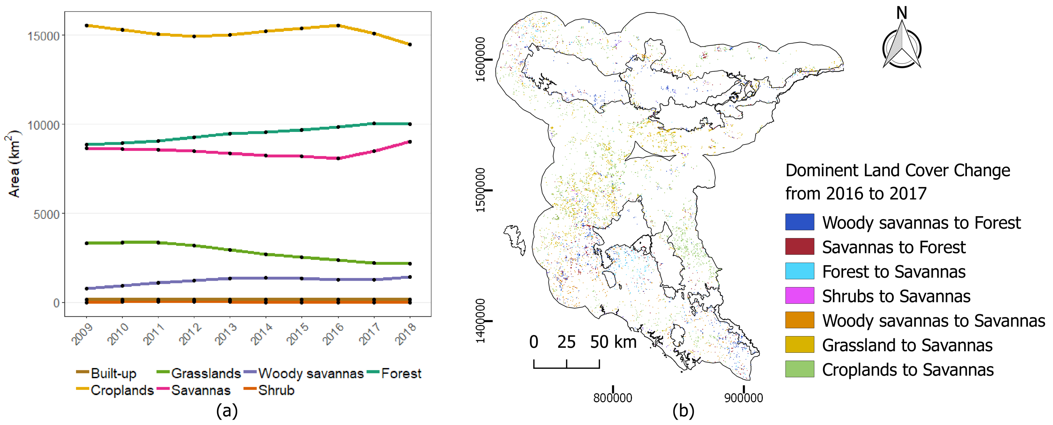
In resource suitability maps, areas with orange color corresponded to a high baseline with moderate negative rate of change in HEC probability. This decreasing trend ( to per year) in both wet and dry season was mainly predicted around the edge of the forests. Base on MODIS land cover (Figure 9), the reduction of HEC probability near the forest was due mainly to forest cover increased over the years. According to the predictors’ responses in Figure 3, areas with high forest densities and nearer to forest were estimated with lower HEC probability. Positive trends (0.2 to 0.4 per year) was sparsely predicted in both wet and dry seasons on the west-side of Ang Ruenai-WS in Chachoengsao and Chantaburi provinces. Although we cannot specify a reason behind this increase, we observed from MODIS land cover that there was an expansion of the savannas land cover during 2017–2018, as well as increased of forest in those areas (Figure 9b). The high HEC probability of EVI slope corresponded to the characteristics of forest and savanna which may have heightened the predicted probability.
For direct human pressure scenario, large areas of increasing trend occurred in previously low and moderate HEC probability baseline in wet (a pure bright blue) and dry (a dark greenish-blue) season respectively. These areas were located around Ang Ruenai-WS, north-east of Khao Yai-NP, and north of Thablan-NP. Since the variables used under direct human pressure scenario only contain static and annual characteristic (Table 1), the differences observed between seasons were not the result of physical differences. The dissimilarities were due to seasonal differences of variable response that governed HEC prediction. In addition, the southern areas of Ang Ruenai-WS were predicted with constantly high HEC probability (around 0.7) from human pressure in the dry season. The increasing trend within the same areas in the wet season (a rate of 0.07 to 0.10 per year) likely caused a year-round HEC. The large positive trend from direct human pressure, when happen in areas with already high HEC probability predicted under resource suitability, may escalate HEC to a higher category. Lastly, spares areas in orange indicated a decreasing trend in HEC probability. These areas scattered in the west near the main roads. This is due to human population growth. The same was not predicted for the dry season because of the differences in variable response between the two models.
4. Discussion
Using two-dimensional classification together with time-calibrated SDM on remotely sensed satellite data, we predicted and compared potential HEC distribution in Eastern Thailand across 20 seasons. Overall, our models predicted the occurrence of large HEC-conflict areas during the dry season which decreased both in term of spatial extent and intensity during the wet season. Chantaburi and Nakhon Ratchasima were predicted to have the largest HEC-prone areas. Drought-induced decrease in the distribution of suitable resources (base on KBDI index), resulted to a relevant decrease in the spatial extent of HEC. The high KBDI detected in 2010 and 2014–2016 (Figure 8) coincided with the El Nino phenomena that caused severe and prolonged drought in Thailand [72]. This caused a decrease in the spatial HEC extent in some provinces, but HEC extent increased in other provinces. Previous studies in arid savannas showed that extreme drought can alter the distribution and abundance of elephants population, leading to mass starvation [73,74]. However, such extreme events is usually not considered during modeling. Considering that dry periods, and their associated extreme drought events, may occur more frequently due to climate change, HEC distribution may become unpredictable, causing critical management implications. Additional field investigation is required to examine whether or not a decrease in the spatial HEC extent in some areas may result to concentrated increase of elephant-induced damages in other locations.
The peak of HEC probability for forest percent cover, a variable with the highest predictive power, was identified at 25%–45%. Forest land cover mainly entailed protected areas. Hence, HEC occurred in areas close to elephant natural habitats. Although high HEC occurrence near protected areas is expected, the peak probability implies that conflict incidents do not always locate directly adjacent to protected parks. Available patches of forest outside of protected areas, such as community forest, may assist in wild elephant dispersal as long as the composition with other land cover provide 25%–45% cover within 6 km. Further field study is necessary to identify the size of forest patches required by elephants outside of protected areas.
HEC hotspots along the southern and western of Ang Ruenai-WS were dominated by savannas land cover, a mixed tree and grass system. The peak in HEC probability as seen from EVI slope coincided with characteristics of MODIS savannas and forest land cover class. By comparing MODIS land cover with land use map from Land Development Department, Ministry of Agriculture and Cooperatives of Thailand, savannas land cover was generally rubber plantations and orchards. Available tree canopies in these land use, despite being sparse, may provide cover for elephants and assist in their movement. Studies in India and China identified proximity to forest edge and high-statue vegetation (e.g., eucalyptus and acacia) as important factors determining elephant occurrences outside of protected areas [25,75,76]. With large continuous extant of savannas within these hotspot, together with high HEC predicted across both season, elephants may already be frequent and even residing permanently in the areas.
Although predictor responses were generally similar to studies from other Asian countries, some variable contributions were different. Distance to water has been identified as an important factor determining elephants distribution in China [25], Indonesia [77], India [78], and Thailand [79]. In this study, however, it was not a prominent predictor. We expected the reason to be the coarse spatial resolution as we re-sampled the data from 30m to 500m. Consequently, small water bodies located in individual farmers’ lands might not be captured. Although vegetation index was a good proxy for forage quality in [44], the EVI variable had relatively lower predictive importance in our study. Usefulness of vegetation index depends highly on the types of habitat and the season [80]. In tropical forest, elephant forage abundance was unable to be mapped directly using average value of NDVI [81]. Nevertheless, EVI slope had the highest predictive power among all EVI variables, implying possible importance of vegetation phenology. A study of crop raiding behavior in African elephants identified crop availability and ripening timing as important indicators for predicting crop damage [82]. Therefore, variables related to crop types along with its phenology, which can be detected from remotely sensed satellite data, should be further studied.
Overall our calibrated models had a good to very good predictive power with AUC ranging from 0.73–0.81. Nevertheless, this study still contains limitations and uncertainties. First, although bias correction was applied, we still cannot account for unreported locations where HEC occurred but not reported in the news. Second, different in variable responses were identified between wet and dry season, but the significance between predicted wet and dry HEC distributions remain to be evaluated. Having two separate HEC maps can support effective operational planning (e.g., seasonal patrol routes), but can also cause difficulty for policy-level planning. Future study can evaluate models from key season similar to [35] in which winter season was chosen. Third, additional variables can be included to provide better prediction of HEC occurrence. Besides potential use of cropping pattern and phenology, human tolerance and perception of risk should also be considered. These factors represent the possibility of coexistence between human and wildlife [16]. Fourth, current mitigation efforts have not been included, but are essential as they can alter elephants’ access to resources. Previous studies have shown that implementation of physical barriers shift HEC to new locations [83]. Such data on existing mitigation can be incorporated after to identify movement routes and potential corridors. Lastly, future study can include assessment of habitat quality within protected areas. Our models predicted an increase in potential HEC areas after prolong drought during 2014–2016. We cannot infer a conclusion based on our current study. However, extreme events can cause a change to land use and vegetation in the following years, impacting elephant’s natural habitat and adjacent agricultural lands. Such information can elucidate root cause of conflict and enhance management decision.
Making informed decision on where to allocate limited resources is crucial for government and conservation organizations alike [84]. A two-dimensional classification approach has been used to identified management-relevant actions in habitat modeling [35,36,37]. Utilizing similar method, we recommended prioritization of HEC-zone dependent management actions. Two groups of management actions are considered, (i) natural resource/land management and (ii) promotion of human adaptation. High HEC zones must receive first priority with parallel emphasis on both land-use policies and human adaptation. Together with HEC-relevant land management, behavioral adaptation of those who live in the areas are important to reduce risky behaviors. In Likely HEC zones, certain land management actions are not necessary (e.g., permanent electric fences), but more focus should be put on community development. For areas with Low HEC category, the extensive change in human behavior may not be needed (e.g crop husbandry), but general knowledge on appropriate actions when encountering with wild elephants are potentially useful. In such areas, land use planning is more important in preventing further escalation of conflict. Lastly, Rare HEC zones were predicted sparsely and far from protected areas (Figure 4). Since these areas were concentrated closer to the main roads, management may focus on the risk of vehicle-elephant-collision. Further field investigation and data collection are necessary to pinpoint appropriate management actions.
5. Conclusions
This study utilized publicly available dataset and applied time-calibrated SDM with two-dimensional conflict classification to estimate time-series distribution of potential HEC in eastern Thailand. We illustrated the impact of inter-annual and seasonal variation on the distribution of potential HEC, as well as distinguished the contribution between resource suitability and direct human pressure. Overall increasing trend of HEC was predicted from 2009 to 2018, with larger extend in the dry season. Large reduction of conflict areas in 2010 and 2014–2016 were likely explained by server drought due to El Nino events which was captured by KBDI. Our results also suggested that variation in probability and distribution of HEC was due to changes in resource suitability, while a more continuously gradual increase was observed from direct human pressure. Besides identifying HEC response to environmental characteristics, our findings can also support prioritization of conservation resources. We recommended HEC-zone dependent management focus. Parallel emphasis on extensive land management and human co-adaptation should be performed in High HEC-zones. In Likely HEC-zones, more attention should be given to raise safe behaviors for communities. Land use policies in Likely HEC-zones should be strengthened with general awareness of appropriate actions when encountering wild elephants. Rare HEC-zones were scattered close to main roads, hence we recommended investigation to prevent vehicle-elephant collision. Within each zone, more priority can be given to hotspots that estimated with repeated HEC. Lastly, this study highlighted the advantages of satellite-derived variables with high temporal resolution which can capture annual and seasonal variation.
Supplementary Materials
The following are available online at https://www.mdpi.com/2072-4292/12/1/90/s1, Figure S1: Histograms of three Enhanced Vegetation Index (EVI) properties.
Author Contributions
N.K. and W.T. conceived and designed the study; N.K. performed data curation; N.K. analyzed the data; W.T. supervised and provided resources; N.K wrote the paper; W.T. reviewed and provided revision suggestions. All authors have read and agreed to the published version of the manuscript.
Funding
This research received no external funding.
Acknowledgments
The authors would like to thank the Department of National Parks, Wildlife and Plant Conservation of Thailand for allowing us to attend a workshop and conduct interviews with park rangers at Khao Yai National Parks. We also thank reviewers and editors whose comments helped improve and clarify this manuscript. This study was in part supported by the Royal Thai Government Scholarship Program.
Conflicts of Interest
The authors declare no conflict of interest.
References
- IUCN/SSC Asian Elephant Specialist Group. Asian Elephant Range States Meeting: Final Report; Technical report; The IUCN Species Survival Commission (SSC): Jakarta, Indonesia, 2017. [Google Scholar]
- Barua, M.; Bhagwat, S.A.; Jadhav, S. The hidden dimensions of human–wildlife conflict: Health impacts, opportunity and transaction costs. Biol. Conserv. 2013, 157, 309–316. [Google Scholar] [CrossRef]
- Rangarajan, M.; Desai, A.; Sukumar, R.; Easa, P.; Menon, V.; Vincent, S.; Ganguly, S.; Talukdar, B.K.; Singh, B.; Mudappa, D.; et al. Gajah: Securing the Future for Elephants in India; Technical report, The Report of the Elephant Task Force; Ministry of Environment and Forests: New Delhi, India, 2010.
- Noonto, B. Managing Human-Elephant Conflict (HEC) Based on Elephant and Human Behaviors: A Case Study at Thong Pha Phum National Park, Kanchanaburi, Thailand. Ph.D. Thesis, Mahidol University, Salaya, Thailand, 2009. [Google Scholar]
- Sukmasuang, R. Human-Elephant Conflict Status and Resolution in Thailand. In Proceedings of the Conference on Biodiversity 2015, Bangkok, Thailand, 10–12 March 2015. [Google Scholar]
- Leimgruber, P.; Gagnon, J.B.; Wemmer, C.; Kelly, D.S.; Songer, M.A.; Selig, E.R. Fragmentation of Asia’s remaining wildlands: Implications for Asian elephant conservation. Animal Conserv. 2003, 6, 347–359. [Google Scholar] [CrossRef] [Green Version]
- Desai, A.A.; Riddle, H.S. Human-Elephant Conflict in Asia; Technical Report; United States Fish and Wildlife Service: Falls Church, VA, USA, 2015. Available online: https://www.fws.gov/international/pdf/Human-Elephant-Conflict-in-Asia-June2015.pdf (accessed on 16 April 2019).
- WCS Thailand. A Manual for Human-Elephant Conflict Mitigation; Saeng Muang Printing: Bangkok, Thailand, 2007; pp. 1–56. [Google Scholar]
- Vinitpornsawan, S. Elephant-Proof Trench. In Wildlife Yearbook 14; Wildlife Research Division, Wildlife Conservation Office, Department of National Parks, Wildlife and Plant Conservation: Bangkok, Thailand, 2012; pp. 195–202. [Google Scholar]
- Salim, S. Collaring Wild Elephants to Save Their Lives. World Wildlife Fund (WWF). 2019. Available online: https://blog.wwf.sg/endangered-species/2019/02/asian-elephant-wild-eastern-thailand/ (accessed on 20 June 2019).
- Nuntatripob, N. Management Solution for Conflict between Human and Wild Elephant; Legislative Institutional Repository of Thailand (LIRT): Bangkok, Thailand, 2019; pp. 1–9. Available online: http://dl.parliament.go.th/backoffice/viewer/viewer.php (accessed on 19 October 2019).
- Saif, O.; Kansky, R.; Palash, A.; Kidd, M.; Knight, A.T. Costs of coexistence: Understanding the drivers of tolerance towards Asian elephants Elephas maximus in rural Bangladesh. Oryx 2019, 1–9. [Google Scholar] [CrossRef]
- Dickman, A.J. Complexities of conflict: The importance of considering social factors for effectively resolving human-wildlife conflict. Animal Conserv. 2010, 13, 458–466. [Google Scholar] [CrossRef]
- Redpath, S.M.; Bhatia, S.; Young, J. Tilting at wildlife: Reconsidering human–wildlife conflict. Oryx 2015, 49, 222–225. [Google Scholar] [CrossRef] [Green Version]
- Nyhus, P.J. Human–Wildlife Conflict and Coexistence. Ann. Rev. Environ. Resour. 2016, 41, 143–171. [Google Scholar] [CrossRef] [Green Version]
- Morzillo, A.T.; de Beurs, K.M.; Martin-Mikle, C.J. A conceptual framework to evaluate human-wildlife interactions within coupled human and natural systems. Ecol. Soc. 2014, 19, 44. [Google Scholar] [CrossRef]
- Shaffer, L.J.; Khadka, K.K.; Van Den Hoek, J.; Naithani, K.J. Human-Elephant Conflict: A Review of Current Management Strategies and Future Directions. Front. Ecol. Evol. 2019, 6, 235. [Google Scholar] [CrossRef] [Green Version]
- Chen, Y.; Marino, J.; Chen, Y.; Tao, Q.; Sullivan, C.D.; Shi, K.; Macdonald, D.W. Predicting Hotspots of Human-Elephant Conflict to Inform Mitigation Strategies in Xishuangbanna, Southwest China. PLoS ONE 2016, 11, e0162035. [Google Scholar] [CrossRef]
- Van de Water, A.; Matteson, K. Human-elephant conflict in western Thailand: Socio-economic drivers and potential mitigation strategies. PLoS ONE 2018, 13, e0194736. [Google Scholar] [CrossRef]
- Jenks, K.E.; Songsasen, N.; Kanchanasaka, B.; Bhumpakphan, N.; Wanghongsa, S.; Leimgruber, P. Community Attitudes toward Protected Areas in Thailand. Nat. Hist. Bull. Siam Soc. 2013, 59, 65–76. [Google Scholar]
- Parr, J.W.K.; Jitvijak, S.; Saranet, S.; Buathong, S. Exploratory co-management interventions in Kuiburi National Park, Central Thailand, including human-elephant conflict mitigation. Int. J. Environ. Sustain. Dev. 2008, 7, 293–310. [Google Scholar] [CrossRef]
- Thongjan, N.; Horayangkura, P.; Sirichalearn, D.; Yanpirat, W.; Chatprapachai, P.; Chongpanish, T.; Chureemas, R. Legal Measures for Managing Areas to Conserve Wild Elephants. CMU J. Law Soc. Sci. 2017, 10, 115–132. [Google Scholar]
- Gubbi, S.; Swaminath, M.H.; Poornesha, H.C.; Bhat, R.; Raghunath, R. An elephantine challenge: human–elephant conflict distribution in the largest Asian elephant population, southern India. Biodivers. Conserv. 2014, 23, 633–647. [Google Scholar] [CrossRef]
- Goswami, V.R.; Medhi, K.; Nichols, J.D.; Oli, M.K. Mechanistic understanding of human-wildlife conflict through a novel application of dynamic occupancy models. Conserv. Biol. 2015, 29, 1100–1110. [Google Scholar] [CrossRef]
- Li, W.; Liu, P.; Guo, X.; Wang, L.; Wang, Q.; Yu, Y.; Dai, Y.; Li, L.; Zhang, L. Human-elephant conflict in Xishuangbanna Prefecture, China: Distribution, diffusion, and mitigation. Glob.Ecol. Conserv. 2018, 16, e00462. [Google Scholar] [CrossRef]
- Elith, J.; Phillips, S.J.; Hastie, T.; Dudík, M.; Chee, Y.E.; Yates, C.J. A statistical explanation of MaxEnt for ecologists. Divers. Distrib. 2011, 17, 43–57. [Google Scholar] [CrossRef]
- Mateo-Tomás, P.; Olea, P.P.; Sánchez-Barbudo, I.S.; Mateo, R. Alleviating human-wildlife conflicts: Identifying the causes and mapping the risk of illegal poisoning of wild fauna. J. Appl. Ecol. 2012, 49, 376–385. [Google Scholar] [CrossRef]
- Sukumar, R. The Asian Elephant: Ecology and Management; Cambridge University Press: Cambridge, UK, 1992. [Google Scholar]
- Santiapillai, C.; Chambers, M.R.; Ishwaran, N. Aspects of the ecology of the Asian elephant Elephas maximus L. in the Ruhuna National Park, Sri Lanka. Biol. Conserv. 1984, 29, 47–61. [Google Scholar] [CrossRef]
- Bedia, J.; Herrera, S.; Gutiérrez, J.M. Dangers of using global bioclimatic datasets for ecological niche modeling. Limitations for future climate projections. Glob. Planet. Chang. 2013, 107, 1–12. [Google Scholar] [CrossRef] [Green Version]
- He, K.S.; Bradley, B.A.; Cord, A.F.; Rocchini, D.; Tuanmu, M.N.; Schmidtlein, S.; Turner, W.; Wegmann, M.; Pettorelli, N. Will remote sensing shape the next generation of species distribution models? Remote Sens. Ecol. Conserv. 2015, 1, 4–18. [Google Scholar] [CrossRef] [Green Version]
- Tuanmu, M.N.; Viña, A.; Roloff, G.J.; Liu, W.; Ouyang, Z.; Zhang, H.; Liu, J. Temporal transferability of wildlife habitat models: Implications for habitat monitoring. J. Biogeogr. 2011, 38, 1510–1523. [Google Scholar] [CrossRef]
- Alabia, I.D.; Dehara, M.; Saitoh, S.I.; Hirawake, T. Seasonal habitat patterns of Japanese common squid (Todarodes pacificus) inferred from satellite-based species distribution models. Remote Sens. 2016, 8, 921. [Google Scholar] [CrossRef] [Green Version]
- Naves, J.; Wiegand, T.; Revilla, E.; Delibes, M. Endangered Species Constrained by Natural and Human Factors: the Case of Brown Bears in Northern Spain. Conserv. Biol. 2003, 17, 1276–1289. [Google Scholar] [CrossRef] [Green Version]
- Bleyhl, B.; Sipko, T.; Trepet, S.; Bragina, E.; Leitão, P.J.; Radeloff, V.C.; Kuemmerle, T. Mapping seasonal European bison habitat in the Caucasus Mountains to identify potential reintroduction sites. Biol. Conserv. 2015, 191, 83–92. [Google Scholar] [CrossRef]
- De Angelo, C.; Paviolo, A.; Wiegand, T.; Kanagaraj, R.; Di Bitetti, M.S. Understanding species persistence for defining conservation actions: A management landscape for jaguars in the Atlantic Forest. Biol. Conserv. 2013, 159, 422–433. [Google Scholar] [CrossRef]
- Romero-Muñoz, A.; Torres, R.; Noss, A.J.; Giordano, A.J.; Quiroga, V.; Thompson, J.J.; Baumann, M.; Altrichter, M.; McBride, R.; Velilla, M.; et al. Habitat loss and overhunting synergistically drive the extirpation of jaguars from the Gran Chaco. Divers. Distrib. 2019, 25, 176–190. [Google Scholar] [CrossRef] [Green Version]
- Thailand Meteorological Department. The Climate of Thailand (1981–2010); Technical report; Thailand Meteorological Department: Bangkok, Thailand, 2015.
- Nounmusig, W. Analysis of rainfall in the eastern Thailand. Int. J. GEOMATE 2018, 14, 150–155. [Google Scholar] [CrossRef]
- Vinitpornsawan, S.; Bunchornratana, K.; Pukhrua, A.; Panyawiwatanakul, R. Population Structure of Wild Elephant in Eastern Forest Complex. In Wildlife Yearbook 15; Wildlife Research Division, Wildlife Conservation Office, Department of National Parks, Wildlife and Plant Conservation: Bangkok, Thailand, 2015; pp. 89–101. [Google Scholar]
- Fay, M.P.; Proschan, M.A. Wilcoxon-Mann-Whitney or t-test? On assumptions for hypothesis tests and multiple interpretations of decision rules. Stat. Surv. 2010, 4, 1–39. [Google Scholar] [CrossRef]
- Gorelick, N.; Hancher, M.; Dixon, M.; Ilyushchenko, S.; Thau, D.; Moore, R. Google Earth Engine: Planetary-scale geospatial analysis for everyone. Remote Sens. Environ. 2017, 202, 18–27. [Google Scholar] [CrossRef]
- R Core Team. R: A Language and Environment for Statistical Computing; R Foundation for Statistical Computing: Vienna, Austria, 2019. [Google Scholar]
- Pettorelli, N.; Vik, J.O.; Mysterud, A.; Gaillard, J.M.; Tucker, C.J.; Stenseth, N.C. Using the satellite-derived NDVI to assess ecological responses to environmental change. Trends Ecol. Evol. 2005, 20, 503–510. [Google Scholar] [CrossRef] [PubMed]
- Bohrer, G.; Beck, P.S.A.; Douglas-hamilton, I. Elephant movement closely tracks precipitation-driven vegetation dynamics in a Kenyan forest- savanna landscape. Mov. Ecol. 2014, 2, 1–12. [Google Scholar] [CrossRef] [PubMed] [Green Version]
- Liu, H.Q.; Huete, A. Feedback based modification of the NDVI to minimize canopy background and atmospheric noise. IEEE Trans. Geosci. Remote Sens. 1995, 33, 457–465. [Google Scholar] [CrossRef]
- Huete, A. A comparison of vegetation indices over a global set of TM images for EOS-MODIS. Remote Sens. Environ. 1997, 59, 440–451. [Google Scholar] [CrossRef]
- Haralick, R.M.; Shanmugam, K.; Dinstein, I. Textural Features for Image Classification. IEEE Trans. Syst. Man Cybern. 1973, SMC-3, 610–621. [Google Scholar] [CrossRef] [Green Version]
- Takeuchi, W.; Darmawan, S.; Shofiyati, R.; Khiem, M.V.; Oo, K.S.; Pimple, U.; Heng, S. Near-Real Time Meteorological Drought Monitoring and Early Warning System for Croplands in Asia. In Proceedings of the 36th Asian Conference on Remote Sensing 2015 (ACRS 2015): Fostering Resilient Growth in Asia, Quezon City, Philippines, 19–23 October 2015; pp. 171–178. [Google Scholar]
- Pekel, J.F.; Cottam, A.; Gorelick, N.; Belward, A.S. High-resolution mapping of global surface water and its long-term changes. Nature 2016, 540, 418–422. [Google Scholar] [CrossRef]
- U.S. Geological Survey. Hole-filled Shuttle Radar Topography Mission (SRTM) for the globe Version 4, available from the CGIAR-CSI SRTM 90m Database. Available online: http://srtm.csi.cgiar.org (accessed on 10 February 2019).
- Elvidge, C.D.; Hsu, F.C.; Baugh, K.E.; Ghosh, T. National trends in satellite-observed lighting 1992–2012. In Global Urban Monitoring and Assessment through Earth Observation; Weng, Q., Ed.; CRC Press: Boca Raton, FL, USA, 2014; pp. 97–119. [Google Scholar]
- Wu, K.; Wang, X. Aligning pixel values of DMSP and VIIRS nighttime light images to evaluate urban dynamics. Remote Sens. 2019, 11, 1463. [Google Scholar] [CrossRef] [Green Version]
- Li, X.; Li, D.; Xu, H.; Wu, C. Intercalibration between DMSP/OLS and VIIRS night-time light images to evaluate city light dynamics of Syria’s major human settlement during Syrian Civil War. Int. J. Remote Sens. 2017, 38, 5934–5951. [Google Scholar] [CrossRef]
- Kramer-Schadt, S.; Niedballa, J.; Pilgrim, J.D.; Schröder, B.; Lindenborn, J.; Reinfelder, V.; Stillfried, M.; Heckmann, I.; Scharf, A.K.; Augeri, D.M.; et al. The importance of correcting for sampling bias in MaxEnt species distribution models. Divers. Distrib. 2013, 19, 1366–1379. [Google Scholar] [CrossRef]
- Merow, C.; Smith, M.J.; Silander, J.A. A practical guide to MaxEnt for modeling species’ distributions: what it does, and why inputs and settings matter. Ecography 2013, 36, 1058–1069. [Google Scholar] [CrossRef]
- Phillips, S.J.; Dudík, M.; Elith, J.; Graham, C.H.; Lehmann, A.; Leathwick, J.; Ferrier, S. Sample selection bias and presence-only distribution models: implications for background and pseudo-absence data. Ecol. Appl. 2009, 19, 181–197. [Google Scholar] [CrossRef] [PubMed] [Green Version]
- Elith, J.; Kearney, M.; Phillips, S. The art of modelling range-shifting species. Methods Ecol. Evol. 2010, 1, 330–342. [Google Scholar] [CrossRef]
- Fourcade, Y.; Engler, J.O.; Rödder, D.; Secondi, J. Mapping Species Distributions with MAXENT Using a Geographically Biased Sample of Presence Data: A Performance Assessment of Methods for Correcting Sampling Bias. PLoS ONE 2014, 9, e97122. [Google Scholar] [CrossRef] [Green Version]
- Phillips, S.J.; Anderson, R.P.; Schapire, R.E. Maximum entropy modeling of species geographic distributions. Ecol. Model. 2006, 190, 231–259. [Google Scholar] [CrossRef] [Green Version]
- Elith, J.; Graham, C.H. Do they? How do they? WHY do they differ? On finding reasons for differing performances of species distribution models. Ecography 2009, 32, 66–77. [Google Scholar] [CrossRef]
- Hijmans, R.J.; Phillips, S.; Leathwick, J.; Maintainer, J.E. Package ‘dismo’. Species Distribution Modeling. 2017. Available online: http://cran.r-project.org/web/packages/dismo/index.html (accessed on 18 November 2019).
- Sieber, A.; Uvarov, N.V.; Baskin, L.M.; Radeloff, V.C.; Bateman, B.L.; Pankov, A.B.; Kuemmerle, T. Post-Soviet land-use change effects on large mammals’ habitat in European Russia. Biol. Conserv. 2015, 191, 567–576. [Google Scholar] [CrossRef]
- Muscarella, R.; Galante, P.J.; Soley-Guardia, M.; Boria, R.A.; Kass, J.M.; Uriarte, M.; Anderson, R.P. ENMeval: An R package for conducting spatially independent evaluations and estimating optimal model complexity for Maxent ecological niche models. Methods Ecol. Evol. 2014, 5, 1198–1205. [Google Scholar] [CrossRef]
- Liu, C.; Newell, G.; White, M. On the selection of thresholds for predicting species occurrence with presence-only data. Ecol. Evol. 2016, 6, 337–348. [Google Scholar] [CrossRef] [PubMed] [Green Version]
- Radosavljevic, A.; Anderson, R.P. Making better MaxEnt models of species distributions: complexity, overfitting and evaluation. J. Biogeogr. 2014, 41, 629–643. [Google Scholar] [CrossRef]
- Liu, C.; White, M.; Newell, G. Selecting thresholds for the prediction of species occurrence with presence-only data. J. Biogeogr. 2013, 40, 778–789. [Google Scholar] [CrossRef]
- Neupane, D.; Johnson, R.L.; Risch, T.S. How do land-use practices affect human—elephant conflict in nepal? Wildl. Biol. 2017, 2017, wlb.00313. [Google Scholar] [CrossRef] [Green Version]
- Goswami, V.R.; Vasudev, D. Triage of Conservation Needs: The Juxtaposition of Conflict Mitigation and Connectivity Considerations in Heterogeneous, Human-Dominated Landscapes. Front. Ecol. Evol. 2017, 4. [Google Scholar] [CrossRef] [Green Version]
- Chen, S.; Yi, Z.F.; Campos-Arceiz, A.; Chen, M.Y.; Webb, E.L. Developing a spatially-explicit, sustainable and risk-based insurance scheme to mitigate human–wildlife conflict. Biol. Conserv. 2013, 168, 31–39. [Google Scholar] [CrossRef]
- Treves, A.; Wallace, R.B.; Naughton-Treves, L.; Morales, A. Co-Managing Human–Wildlife Conflicts: A Review. Hum. Dimens. Wildl. 2006, 11, 383–396. [Google Scholar] [CrossRef]
- NOAA/National Weather Service. Historical El Nino / La Nina episodes (1950–present). 2019. Available online: https://origin.cpc.ncep.noaa.gov/products/analysis_monitoring/ensostuff/ONI_v (accessed on 24 September 2019).
- Wato, Y.A.; Heitkönig, I.M.A.; van Wieren, S.E.; Wahungu, G.; Prins, H.H.T.; van Langevelde, F. Prolonged drought results in starvation of African elephant (Loxodonta africana). Biol. Conserv. 2016, 203, 89–96. [Google Scholar] [CrossRef]
- Foley, C.; Pettorelli, N.; Foley, L. Severe drought and calf survival in elephants. Biol. Lett. 2008, 4, 541–544. [Google Scholar] [CrossRef] [Green Version]
- Kumar, M.A.; Mudappa, D.; Raman, T.R.S. Asian Elephant Elephas Maximus Habitat Use and Ranging in Fragmented Rainforest and Plantations in the Anamalai Hills, India. Trop. Conserv. Sci. 2010, 3, 143–158. [Google Scholar] [CrossRef] [Green Version]
- Liu, P.; Wen, H.; Lin, L.; Liu, J.; Zhang, L. Habitat evaluation for Asian elephants (Elephas maximus) in Lincang: Conservation planning for an extremely small population of elephants in China. Biol. Conserv. 2016, 198, 113–121. [Google Scholar] [CrossRef]
- Evans, L.J.; Asner, G.P.; Goossens, B. Protected area management priorities crucial for the future of Bornean elephants. Biol. Conserv. 2018, 221, 365–373. [Google Scholar] [CrossRef]
- Lakshminarayanan, N.; Karanth, K.K.; Goswami, V.R.; Vaidyanathan, S.; Karanth, K.U. Determinants of dry season habitat use by Asian elephants in the Western Ghats of India. J. Zool. 2016, 298, 169–177. [Google Scholar] [CrossRef]
- Meijer, J.R.; Huijbregts, M.A.J.; Schotten, K.C.G.J.; Schipper, A.M. Global patterns of current and future road infrastructure. Environ. Res. Lett. 2018, 13. [Google Scholar] [CrossRef] [Green Version]
- Borowik, T.; Pettorelli, N.; Sönnichsen, L.; Jȩdrzejewska, B. Normalized difference vegetation index (NDVI) as a predictor of forage availability for ungulates in forest and field habitats. Eur. J. Wildl. Res. 2013, 59, 675–682. [Google Scholar] [CrossRef]
- Gautam, H.; Arulmalar, E.; Kulkarni, M.R. NDVI is not reliable as a surrogate of forage abundance for a large herbivore in tropical forest habitat. Biotropica 2019, 51, 443–456. [Google Scholar] [CrossRef]
- Branco, P.S.; Merkle, J.A.; Pringle, R.M.; Pansu, J.; Potter, A.B.; Reynolds, A.; Stalmans, M.; Long, R.A. Determinants of elephant foraging behaviour in a coupled natural system : Is brown the new green ? J. Animal Ecol. 2019, 88, 780–792. [Google Scholar] [CrossRef]
- Osipova, L.; Okello, M.M.; Njumbi, S.J.; Ngene, S.; Western, D.; Hayward, M.W.; Balkenhol, N. Fencing solves human-wildlife conflict locally but shifts problems elsewhere: A case study using functional connectivity modelling of the African elephant. J. Appl. Ecol. 2018, 55, 2673–2684. [Google Scholar] [CrossRef]
- Bottrill, M.C.; Joseph, L.N.; Carwardine, J.; Bode, M.; Cook, C.; Game, E.T.; Grantham, H.; Kark, S.; Linke, S.; McDonald-Madden, E.; et al. Is conservation triage just smart decision making? Trends Ecol. Evol. 2008, 23, 649–654. [Google Scholar] [CrossRef]
Figure 1.
The study area in Eastern Thailand (a). The area is dominated by croplands and savannas, while the damaged villages are located near the forests (b). Human–elephant conflict was modeled within 20-km buffers generated around the nine protected areas (c, d), which are natural habitats for elephant populations.

Figure 2.
Flow chart of the study. Two models for each season under resource availability and direct human pressure were constructed. Projected probability during 2009–2018 were classified and overlaid using proposed conflict category.
Figure 2.
Flow chart of the study. Two models for each season under resource availability and direct human pressure were constructed. Projected probability during 2009–2018 were classified and overlaid using proposed conflict category.
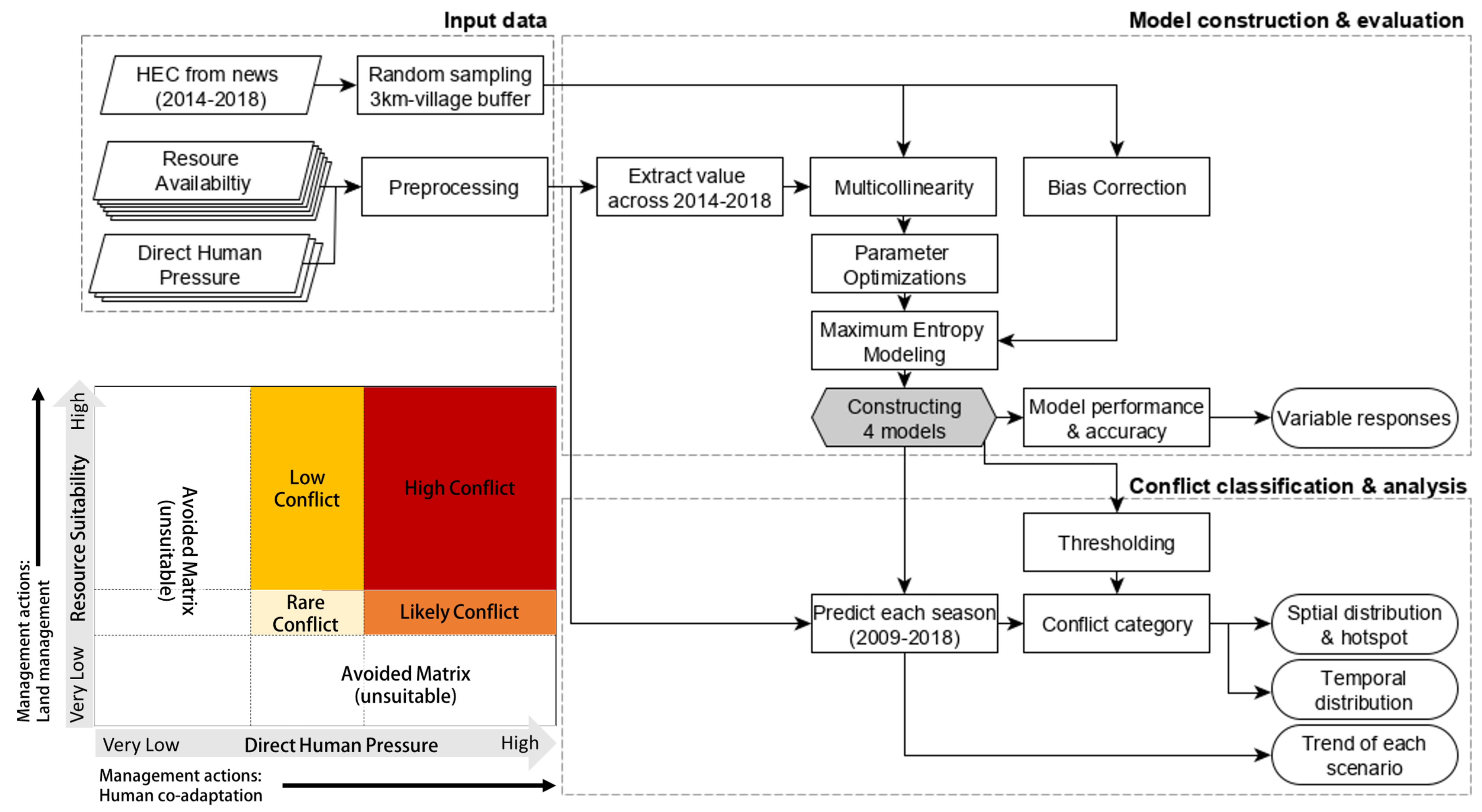
Figure 3.
Relative probability of human–elephant conflict (HEC) occurrences for each environmental predictor, grouped based on resource suitability (top) and direct human pressure (bottom), while keeping all other predictors at average values. The predictors shown had a combined contribution greater than 80%. KBDI, Keetch–Byram Drought Index. EVI, Enhanced Vegetation Index.
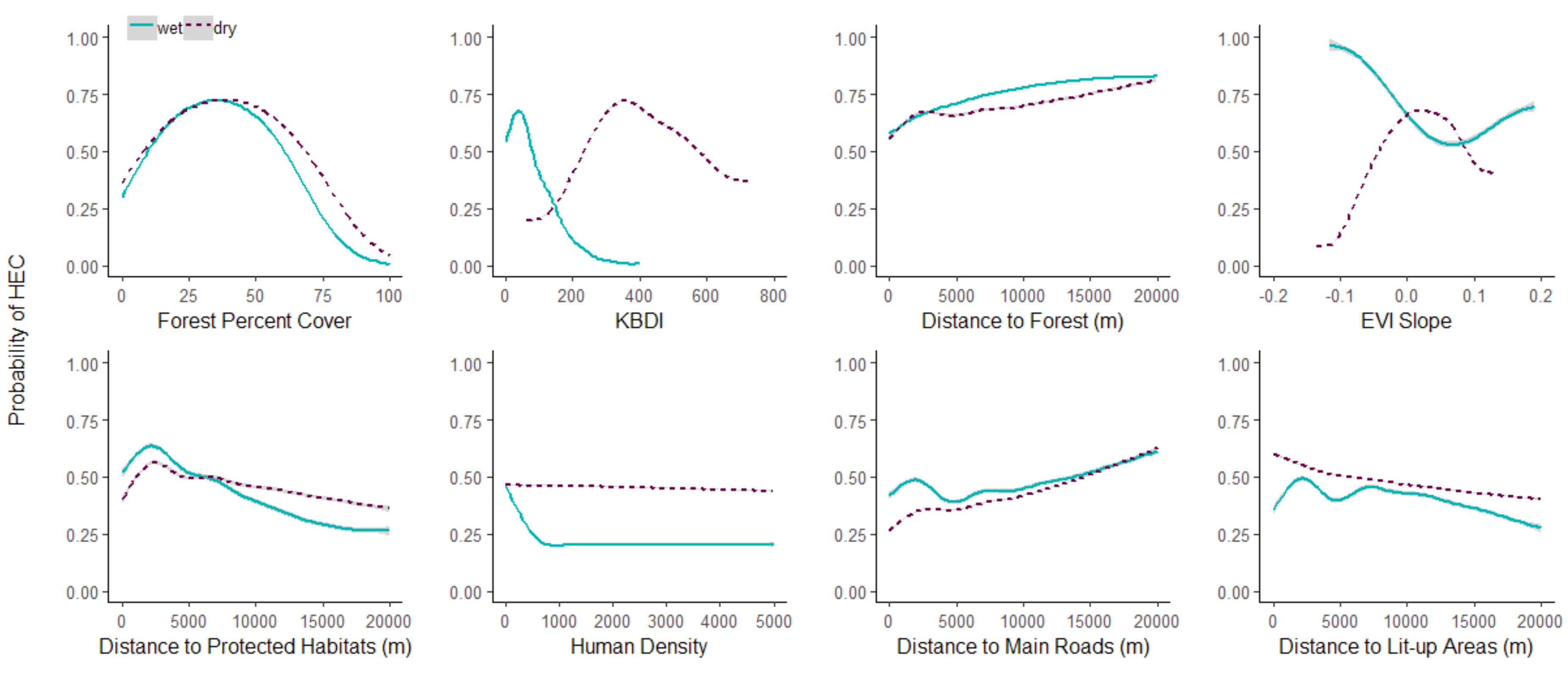
Figure 4.
Conflict probability classes based on the number of years with repeated predictions of human–elephant conflict from 2009 to 2018.
Figure 4.
Conflict probability classes based on the number of years with repeated predictions of human–elephant conflict from 2009 to 2018.

Figure 5.
Total areas of human–elephant conflict under each category showed an overall increasing trend from 2009 to 2018 with larger affected areas under High category in the dry season.
Figure 5.
Total areas of human–elephant conflict under each category showed an overall increasing trend from 2009 to 2018 with larger affected areas under High category in the dry season.
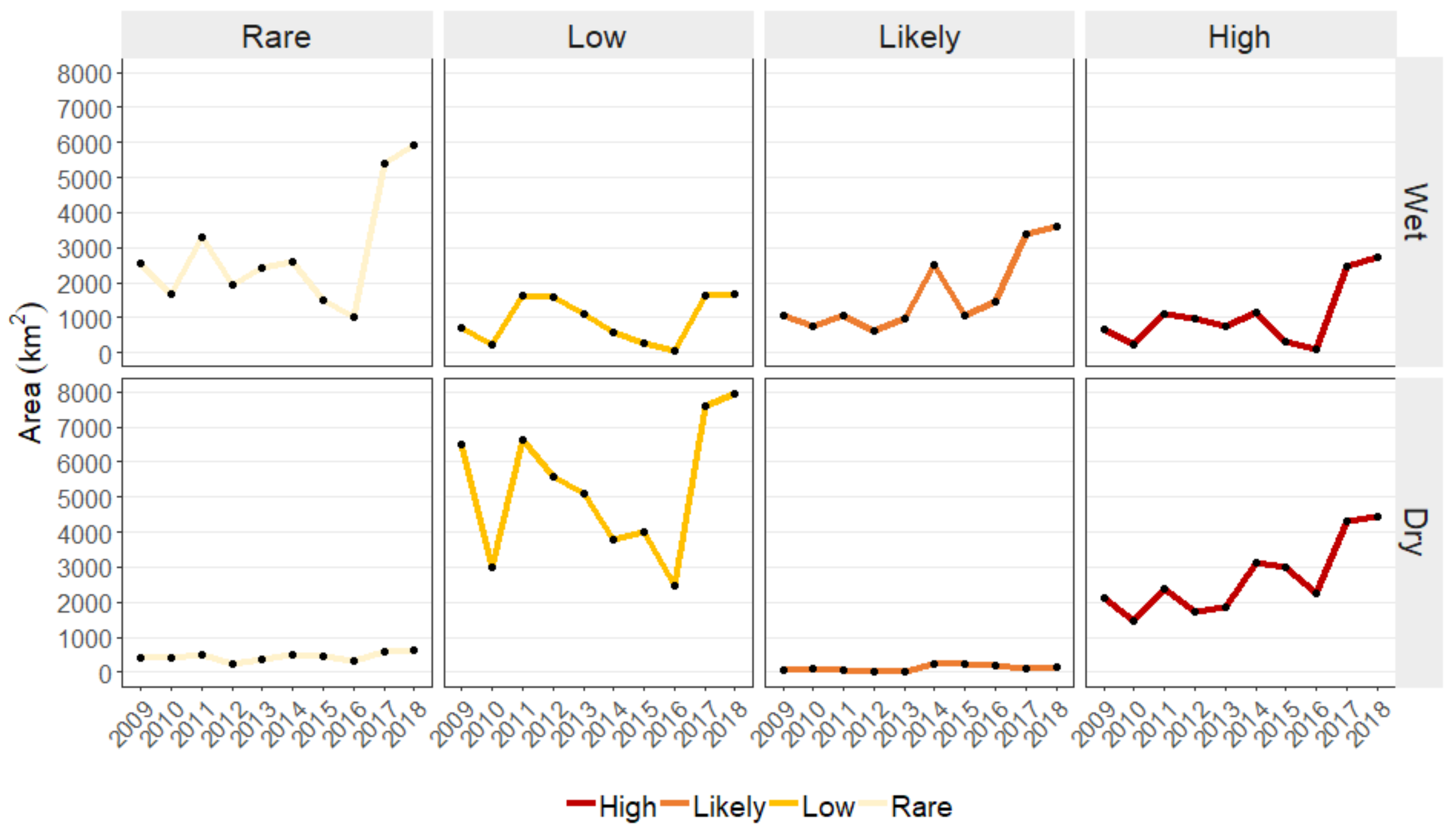
Figure 6.
Areas of human–elephant conflict (HEC) from each category calculated by province from 2009 to 2018 showed that Chantaburi had the largest HEC areas and the expansion of HEC zones was observed in 2017 for most provinces.
Figure 6.
Areas of human–elephant conflict (HEC) from each category calculated by province from 2009 to 2018 showed that Chantaburi had the largest HEC areas and the expansion of HEC zones was observed in 2017 for most provinces.

Figure 7.
(a) Temporal distribution of areas predicted as High, Low, and Very Low category during 2009–2018. (b) Changes in HEC probability from 2009 to 2018 under resource suitability and direct human pressure scenarios. Each location presents two values, a slope and an intercept. The maps are visualized using RGB composite, Red: negative slope (decreasing trend), Green: intercept (baseline of HEC probability in 2009), and Blue: positive slope (increasing trend).
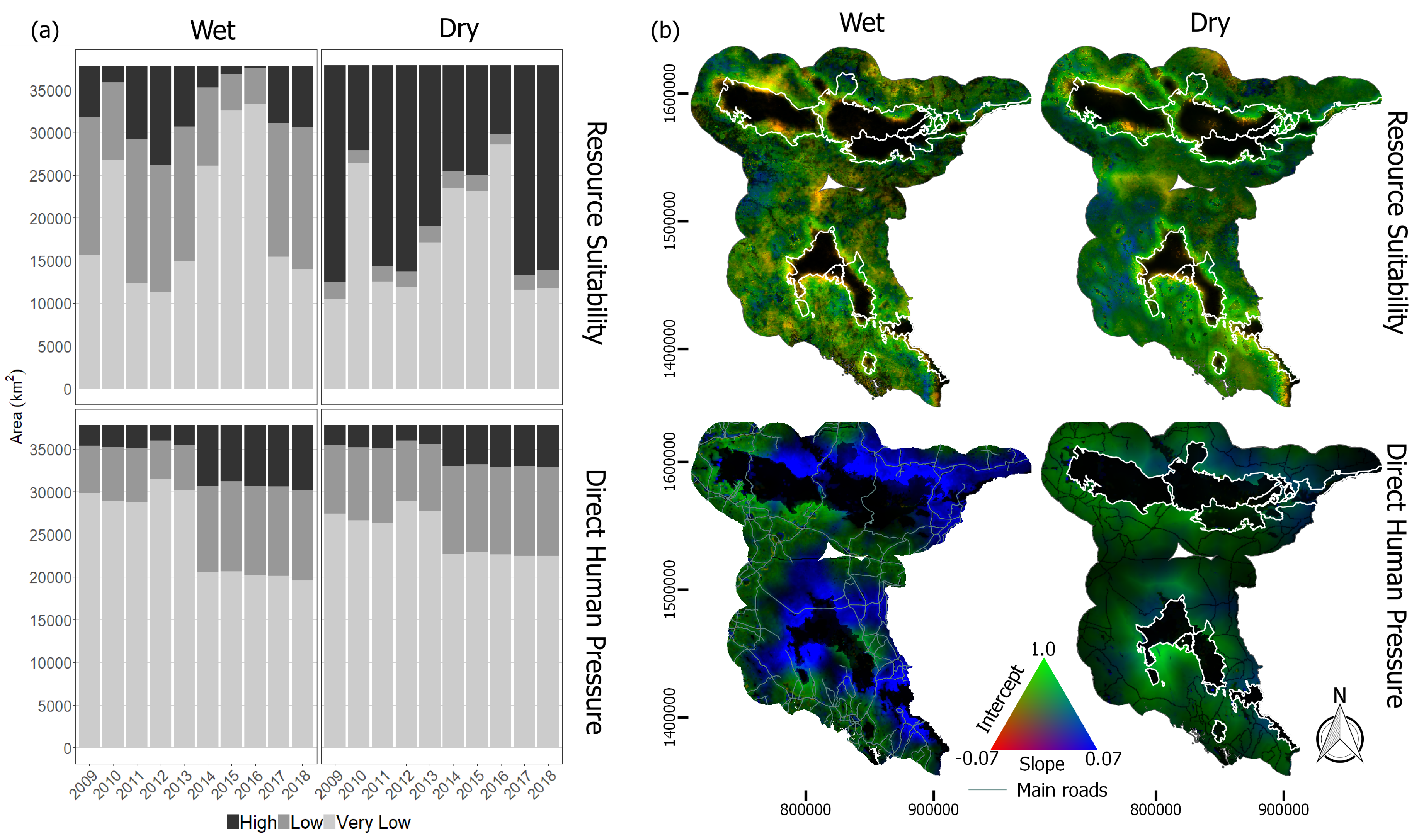
Figure 8.
Anomaly of Keetch–Byram Drought Index (KBDI) showed large positive value in 2014–2016 compared to relatively normal condition in 2013. Positive KBDI anomaly indicated deficit of soil moisture, which is suspected to restrict the availability of resources and alter the potential HEC distribution.

Figure 9.
(a) Areas of different land cover types from 2009 to 2018 based on the reclassified MODIS land cover classes (b) Dominant land cover changes detected from 2016 to 2017.
Figure 9.
(a) Areas of different land cover types from 2009 to 2018 based on the reclassified MODIS land cover classes (b) Dominant land cover changes detected from 2016 to 2017.

Table 1.
List of predictor variables including data source, spatial resolution, and temporal scale in which data was prepared (temporal scale: An—Annual, Se—Seasonal, St—Static).
Table 1.
List of predictor variables including data source, spatial resolution, and temporal scale in which data was prepared (temporal scale: An—Annual, Se—Seasonal, St—Static).
| Variable | Source | Resolution | |
|---|---|---|---|
| Resource-related | |||
| Keetch–Byram Drought Index (KBDI) | KBDI product | 4000 m | Se |
| Enhance Vegetation Index (EVI) | MOD09A1 | 500 m | Se |
| EVI change slope | MOD09A1 | 500 m | Se |
| EVI standard deviation | MOD09A1 | 500 m | Se |
| EVI landscape heterogeneity | MOD09A1 | 500 m | Se |
| Distance to forest | MCD12A1 | 500 m | An |
| Forest percent cover | MCD12A1 | 500 m | An |
| Distance to Water | Global Water Surface product | 30 m | An |
| Terrain Roughness Index (TRI) | SRTM | 90 m | St |
| Direct human pressure | |||
| Distance to lit-up areas | Intercalibrated DMSP and VIIRS | 1000 m | An |
| Human population density | Landscan product | 1000 m | An |
| Distance to main roads | Thailand Bureau of Highway | vector | St |
| Distance to protected habitats | WDPA | vector | St |
© 2019 by the authors. Licensee MDPI, Basel, Switzerland. This article is an open access article distributed under the terms and conditions of the Creative Commons Attribution (CC BY) license (http://creativecommons.org/licenses/by/4.0/).
Share and Cite
MDPI and ACS Style
Kitratporn, N.; Takeuchi, W. Spatiotemporal Distribution of Human–Elephant Conflict in Eastern Thailand: A Model-Based Assessment Using News Reports and Remotely Sensed Data. Remote Sens. 2020, 12, 90. https://doi.org/10.3390/rs12010090
AMA Style
Kitratporn N, Takeuchi W. Spatiotemporal Distribution of Human–Elephant Conflict in Eastern Thailand: A Model-Based Assessment Using News Reports and Remotely Sensed Data. Remote Sensing. 2020; 12(1):90. https://doi.org/10.3390/rs12010090
Chicago/Turabian StyleKitratporn, Nuntikorn, and Wataru Takeuchi. 2020. "Spatiotemporal Distribution of Human–Elephant Conflict in Eastern Thailand: A Model-Based Assessment Using News Reports and Remotely Sensed Data" Remote Sensing 12, no. 1: 90. https://doi.org/10.3390/rs12010090
Note that from the first issue of 2016, this journal uses article numbers instead of page numbers. See further details here.