Mapping Paddy Fields in Japan by Using a Sentinel-1 SAR Time Series Supplemented by Sentinel-2 Images on Google Earth Engine

1
Center for Global Environmental Research, National Institute for Environmental Studies, 16-2 Onogawa, Tsukuba, Ibaraki 305-8506, Japan
2
Graduate School of Agricultural Science, Tohoku University, 468-1 Aoba, Aramaki, Aoba-ku, Sendai, Miyagi 980-8572, Japan
*
Author to whom correspondence should be addressed.
Remote Sens. 2020, 12(10), 1622; https://doi.org/10.3390/rs12101622
Submission received: 27 April 2020
/
Revised: 14 May 2020
/
Accepted: 18 May 2020
/
Published: 19 May 2020
Abstract
:Paddy fields play very important environmental roles in food security, water resource management, biodiversity conservation, and climate change. Therefore, reliable broad-scale paddy field maps are essential for understanding these issues related to rice and paddy fields. Here, we propose a novel paddy field mapping method that uses Sentinel-1 synthetic aperture radar (SAR) time series that are robust for cloud cover, supplemented by Sentinel-2 optical images that are more reliable than SAR data for extracting irrigated paddy fields. Paddy fields were provisionally specified by using the Sentinel-1 SAR data and a conventional decision tree method. Then, an additional mask using water and vegetation indexes based on Sentinel-2 optical images was overlaid to remove non-paddy field areas. We used the proposed method to develop a paddy field map for Japan in 2018 with a 30 m spatial resolution. The producer’s accuracy of this map (92.4%) for non-paddy reference agricultural fields was much higher than that of a map developed by the conventional method (57.0%) using only Sentinel-1 data. Our proposed method also reproduced paddy field areas at the prefecture scale better than existing paddy field maps developed by a remote sensing approach.

1. Introduction
Rice is a staple food for billions of people especially in Asia, and paddy fields play important environmental roles by regulating water and energy budgets and supporting local biodiversity [1,2,3]. Paddy fields have also cultural and esthetic values, as several traditional ones were awarded as Globally Important Agricultural Heritage [4]. In addition, paddy fields are remarkable with respect to global warming because they are a major source of methane (CH4), the second most influential greenhouse gas for global warming following CO2. According to the fifth assessment report of the Intergovernmental Panel on Climate Change, global emissions from paddy fields are estimated to be 33 to 40 Tg (CH4)/yr, or approximately 12% of total anthropogenic methane emissions [5]. In Japan, however, methane emissions from paddy fields account for more than 45% of total anthropogenic methane emissions [6]. Thus, regional methane budgets strongly depend on the paddy field distribution. High-accuracy mapping of broad-scale paddy fields is of fundamental importance for understanding these issues related to rice and paddy fields.
Satellite remote sensing is often the most appropriate approach for a comprehensive understanding of land cover. For example, the MCD12Q1 is a global land cover map based on Moderate Resolution Imaging Spectroradiometer (MODIS) data, and the Global Food Security-support Analysis Data Product (GFSAD1000) is a global cropland map based on multi-satellite data (e.g., Landsat, MODIS) [7,8]. With the increasing necessity of broad-scale paddy field maps in various research fields, many efforts to produce such maps have used satellite remote sensing images, including both optical images and synthetic aperture radar (SAR) images. Before the early 2010s, most research on broad-scale paddy field mapping used remote sensing images with low to medium spatial resolutions, such as MODIS (250 to 1000 m spatial resolutions) [9,10,11,12,13,14,15,16]. Processing of multi-source remote sensing images at high spatial resolutions, such as Landsat (30 m spatial resolution), on a broad scale, is a major challenge because it requires a high computer operating capacity and large amounts of storage. Until recently few remote sensing images have been available free of charge or at a low price, broad-scale paddy field mapping has been very expensive. For this reason, various mapping techniques based on limited remote sensing resources have been developed to improve the accuracy of paddy field mapping. For example, the land surface water index (LSWI), normalized difference vegetation index (NDVI), and enhanced vegetation index (EVI), based on multispectral optical images, have been effectively used to extract irrigated paddy fields [9,10,11,12,13,14], and optical images from multiple sources have also been used to improve classification accuracy [15,16].
In recent years, many remote sensing analyses have utilized cloud-based platforms [17,18,19]. In particular, Google Earth Engine (GEE) is a popular cloud-based platform for broad-scale geospatial analyses. With GEE, high-performance computing resources for the processing of very large geospatial datasets can be accessed without the necessity to provide in-house information technology support [20]. Therefore, GEE solves many difficulties associated with broad-scale remote sensing analyses and makes it possible to use huge numbers of multisource remote sensing images with high spatial resolution. For example, Dong et al. [17], using over a thousand scenes of Landsat 8 images on GEE, have developed a paddy field map for northeastern Asia with a 30 m spatial resolution. The spatial resolution of this paddy field map is much finer than that of conventional paddy field maps developed by using low spatial resolution satellite images.
However, only a few broad-scale paddy field maps have been developed to date because some serious technical issues remain. For example, rice cultivation periods roughly overlap with rainy and cloudy seasons, and they differ among regions depending on factors such as the rice cultivar and the water management practice used. To solve these issues, several methods that use SAR images have been proposed, because SAR images can be obtained even under cloudy conditions. Among the many kinds of SAR images, Sentinel-1 images are used often because they are open source and have high spatial and temporal resolution [19,21,22,23,24,25,26,27,28,29,30]. However, methods that use only Sentinel-1 images have low accuracy for paddy field extraction, because the backscatter of Sentinel-1 is less sensitive to vegetation and irrigated agricultural areas than multi-band optical sensors [21].
In this study, to compensate for this weakness of Sentinel-1 time series images for broad-scale paddy field mapping, we propose a novel paddy field mapping method that supplements the use of Sentinel-1 time series images with Sentinel-2 optical images to reduce misclassification of land covers. The proposed method is more reliable and robust for the extraction of irrigated areas across various land surface types. We developed two sets of paddy field maps with a 30 m spatial resolution for Japan in 2018. We developed one set by using a conventional method based on only Sentinel-1 time series images, and we developed the other set by using our proposed method based on Sentinel-1 time series images supplemented by Sentinel-2 images. Then, by comparing the results obtained by the two methods, we showed that our proposed method improved the paddy field mapping accuracy. Then, we compared the paddy field maps developed by our method with two major existing paddy field maps to demonstrate the potential of our method for accurate broad-scale paddy field mapping.
2. Materials and Methods
2.1. Study Area
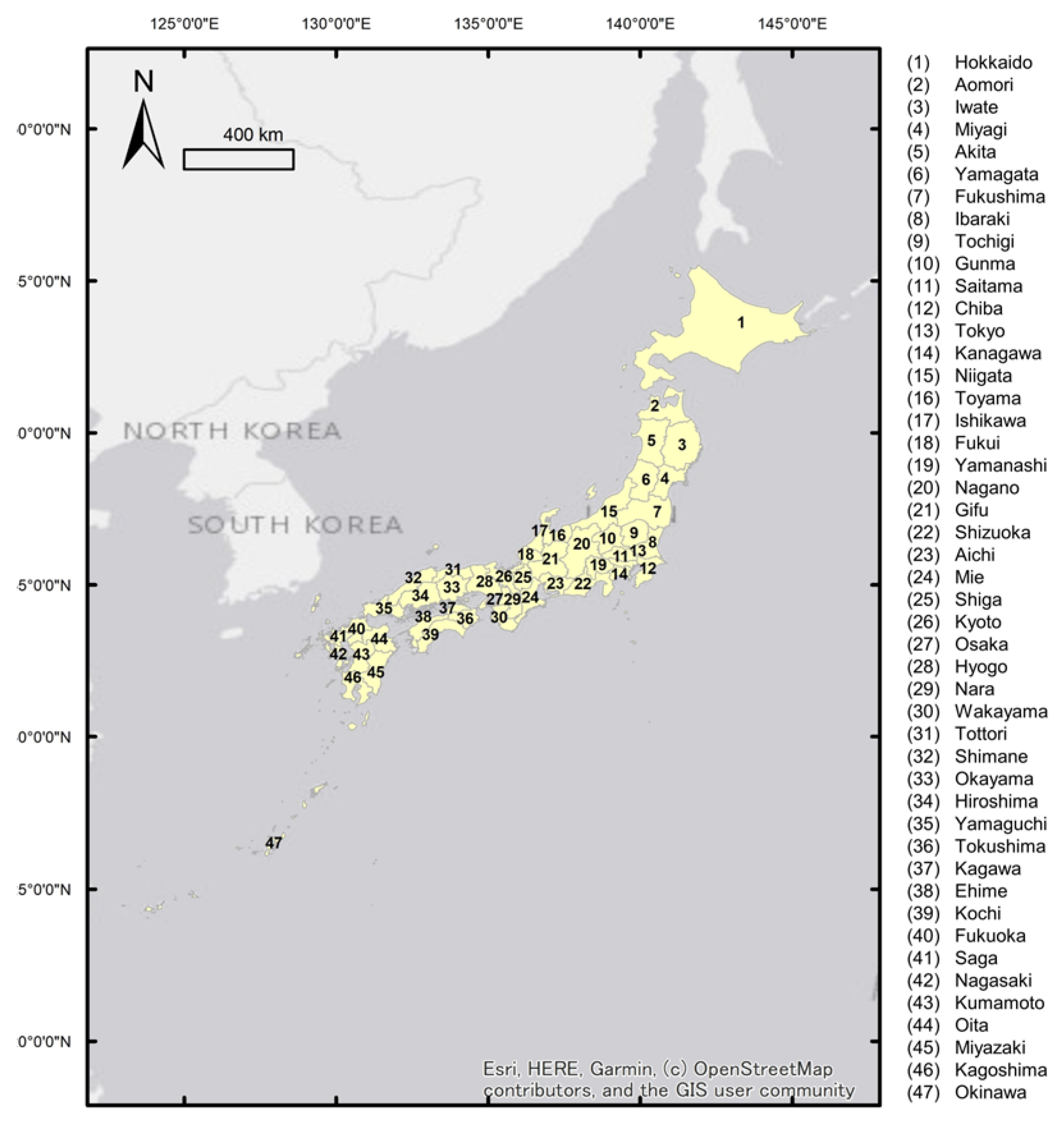
The whole area of Japan (20–46°N, 123–154°E), comprising 47 prefectures, was selected as the study area (Figure A1 in Appendix A). According to the FAO, in 2018 Japan was the 13th largest rice producer in the world [31], and according to the Ministry of Agriculture, Forestry, and Fisheries of Japan (MAFF), the total paddy field area in 2018 planted to rice, including both food rice and feed rice, was approximately 15,920 km², and approximately 7.8 million tons of food rice was produced in that year [32]. In most paddy fields in Japan, single rice cropping with irrigation is practiced. However, in Okinawa prefecture, the southernmost prefecture of Japan, double rice cropping with irrigation, which means two rice crops on a field in a single year, is practiced in a very small area (total 1.89 km²). The area accounted for only 0.012% of the total paddy field area in Japan, and we aimed to develop a paddy field mapping method applicable to all irrigated paddy fields, so no further categorization of irrigated paddy fields was done.
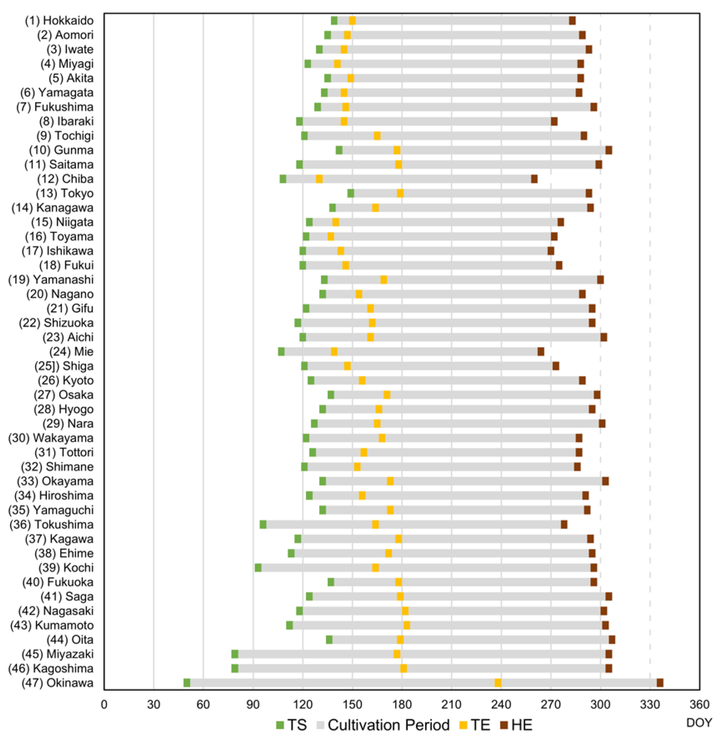
Until 2017, MAFF published typical rice cultivation dates for each prefecture, including “Transplant Start ” (TS), “Transplant End” (TE), and “Harvest End” (HE) dates [33], where TS and TE are the dates on which 5% and 95%, respectively, of the total paddy field area has been transplanted, and HE is the date on which 95% of the total paddy field area has been harvested. We used the average day of the year (DOY) calculated using the TS, TE, and HE dates for the three years from 2015 to 2017 in our analysis (Figure 1).
2.2. Satellite Data
2.2.1. Sentinel-1 Time Series
Sentinel-1 Ground Range Detected (GRD) images were used as fundamental data for our paddy field mapping method because the C-band SAR instrument of Sentinel-1 can obtain data through cloud cover. Sentinel-1 GRD images are thus particularly appropriate for paddy field mapping in Japan, where the rainy season overlaps with the rice cultivation period. Characteristics of the satellite data used in this study are shown in Table 1. The Sentinel-1 satellites were launched by the European Space Agency (ESA) on 3 April 2014 (Sentinel-1A) and 25 April 2016 (Sentinel-1B) [34]. The SAR sensors onboard the Sentinel-1 satellites acquire C-band images at 5.4 GHz in four modes with different spatial resolutions and swath widths. We used the images acquired in Interferometric Wide Swath mode, which acquires images with a swath width of 250 km and a 10 m spatial resolution. To minimize the effects of orbit direction and look angle, for all prefectures except Okinawa prefecture, we used only images that were acquired by the Sentinel-1A satellite during descending orbits in our analysis. For Okinawa prefecture, we used images acquired by the Sentinel-1B satellite during ascending orbits. We used only VH (vertical transmit and horizontal receive) polarized images because some studies have shown that VH-polarized backscatter is more sensitive to rice growth and phenology than other polarizations [22,23]. Both Sentinel-1 satellites have a 12-day revisit cycle at the equator. Therefore, most of the study area is observed about 30 times per year. Using GEE, we accessed all Sentinel-1 GRD images (1073 images) covering the period from 1 January 2018, to 31 December 2018.
2.2.2. Sentinel-2 Multispectral Imager
Sentinel-2 Multispectral Imager (MSI) images were used in a supplemental role for the extraction of paddy fields because they are more reliable and robust for extracting irrigated areas. The Sentinel-2 satellites were launched by the ESA on 23 June 2015 (Sentinel-2A) and 7 March 2017 (Sentinel-2B) [34]. Both satellites have a 10-day revisit cycle. Therefore, most of the study area is observed more than 60 times per year. The Sentinel-2 satellites carry the Sentinel-2 MSI, which is an optical sensor with 12 bands for acquiring images with a swath width of 290 km and a spatial resolution of 10–60 m. We accessed Sentinel-2 MSI Level-1C Top of Atmosphere (TOA) reflectance images (49,694 images) acquired during the irrigated period (from 19 February 2018, to 25 September 2018) by both Sentinel-2A and Sentinel-2B satellites from GEE. Here, the irrigated period is defined as the period from TS to the date calculated by adding 30 days to TE.
2.3. Reference Agricultural Fields
Two classes of reference fields, “Paddy” and “Not paddy”, were prepared for accuracy assessments; here, “Not paddy” reference fields are agricultural fields other than paddy fields.
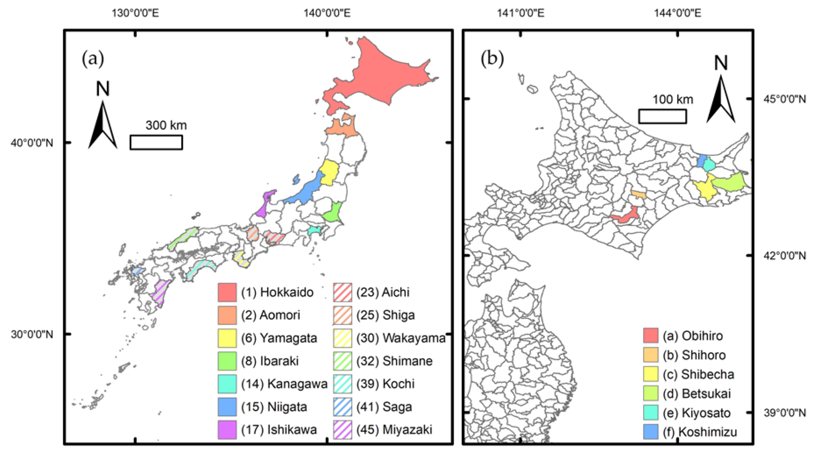
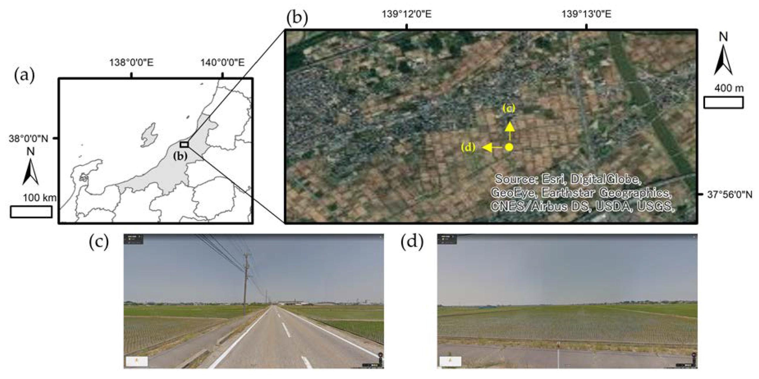
For “Paddy” reference fields, 100 paddy fields were selected from each of 14 prefectures by using Google Maps Street View (Figure 2a), which is being increasingly used for acquiring ground truth data of various land surface types, including agricultural fields [35,36,37]. We selected the 14 prefectures from the 47 prefectures in Japan because Street View data available for the irrigation period in 2018 were limited. However, they effectively covered the whole area of Japan, allowing us to conduct data validation for the present purpose. Further validation including other prefectures remained for our forthcoming study. Irrigation management during the cultivation period of rice is distinctive from that used for other major crops. Therefore, fields that were irrigated and planted to rice could be selected by visual interpretation and designated as “Paddy” reference fields (Figure 3).
For “Not paddy” reference fields, agricultural field polygons derived from high spatial resolution aerial photographs and provided by MAFF were used. Six municipal districts in Hokkaido prefecture (Figure 2b) were selected as “Not paddy” reference field regions. In most of Japan, most cultivated fields are paddy fields, but Hokkaido is atypical because broad areas are used to cultivate grains other than rice, such as wheat, corn, and soybeans. In the six selected districts, no fields were planted to rice in 2018, according to national statistics released by MAFF [32]. Therefore, all agricultural field polygons in the six districts were used as “Not paddy” reference fields.
A total of 1400 field polygons were used as “Paddy” reference fields, and 36,703 field polygons were used as “Not paddy” reference fields.
2.4. Existing Paddy Field Maps
Two different paddy field maps that had been developed by a remote sensing approach were used for accuracy assessment. The first map was produced by Takeuchi and Yasuoka [15,16] from MODIS and Advanced Spacebourne Thermal Emission and Reflection Radiometer (ASTER) images obtained in the early 2000s. This map, referred to here as the “TY” map, covers Monsoon Asia (East Asia, Southeast Asia, and part of South Asia) with a 1 km spatial resolution. The second map is a land-use map produced by the Japan Aerospace Exploration Agency (JAXA) from Landsat 8 operational land imager images obtained between 2014 and 2016 [38]. This map, the “JAXA” map, covers the whole area of Japan with a 30 m spatial resolution, and one of its land-use classes is the “paddy field.”
2.5. Methods
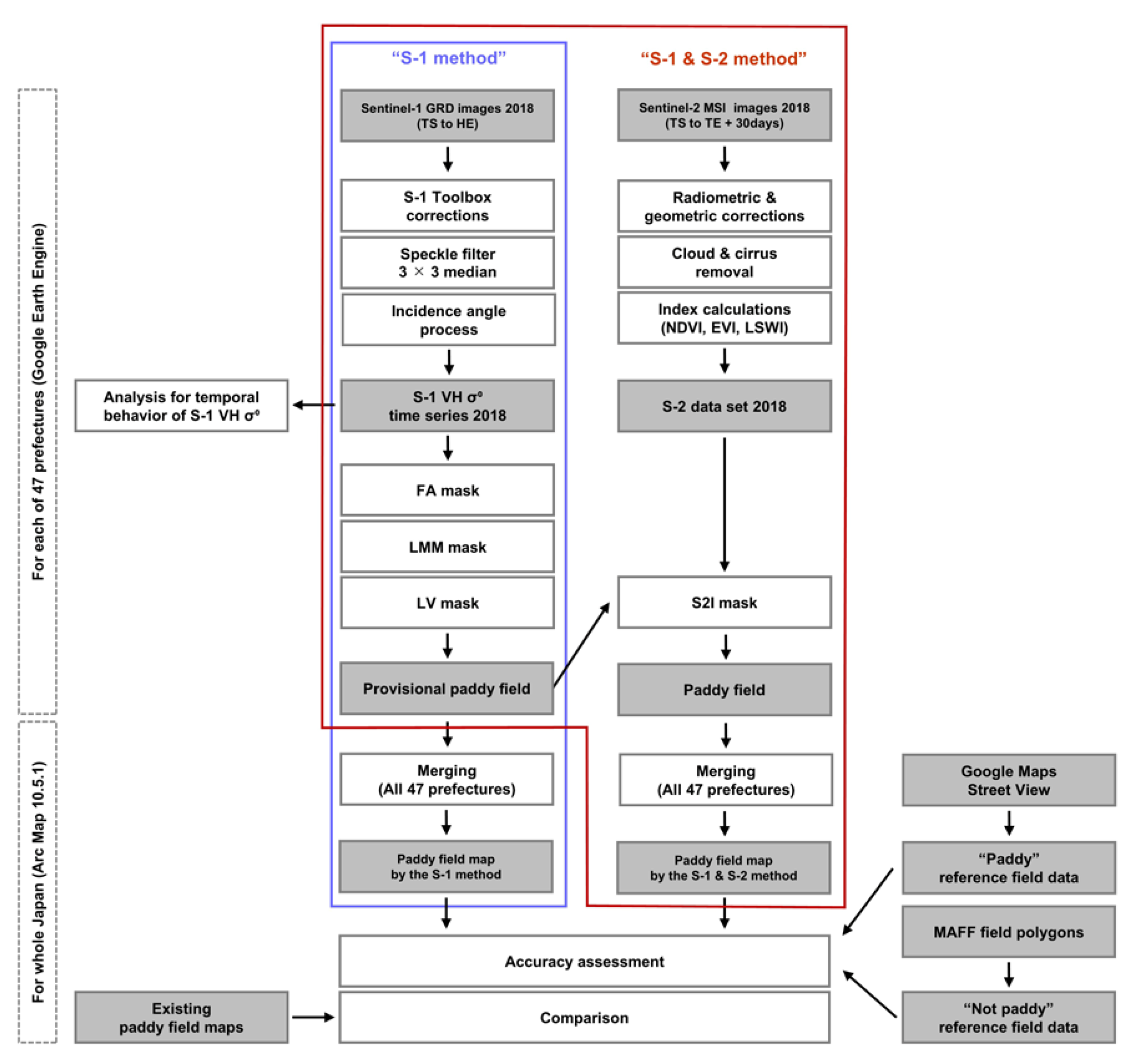
Figure 4 shows a flow chart of the approach used by this study. First, two types of paddy field maps were developed, one by the “S-1” method and the other by the “S-1 & S-2” method. The S-1 method is a conventional paddy field mapping method that uses a decision tree approach and only Sentinel-1 time series data [25,26,27]. The S-1 & S-2 method is our proposed method, which also uses a decision tree approach and Sentinel-1 time series data, but it also uses an additional mask based on Sentinel-2 images. Paddy field maps for each of the 47 prefectures created by each method were merged into a single map for each method covering the whole land area of Japan. All of the processes used to develop the paddy field maps up to the final merging were performed in the GEE platform (https://earthengine.google.com/). The merging, accuracy assessment, and comparison processes were performed in ArcMap 10.5.1.
2.5.1. Preprocessing
To generate the backscatter coefficient (σ0), the Sentinel-1 GRD images accessed on the GEE platform were preprocessed by applying five Sentinel-1 Toolbox corrections developed by the ESA in the following order: (1) orbit file application, (2) ground range detected border noise removal, (3) thermal noise removal, (4) radiometric calibration, and (5) terrain correction. To these preprocessed images, we applied a median filter with a 3 × 3 pixels moving window to reduce inherent speckle noise [24]. In broad-scale analyses of satellite remote sensing images, overlapping observation areas are inevitable. In the case of SAR data, overlapping areas with different incidence angles can produce noise in a time series analysis [19]. Therefore, we applied incidence angle processing to overlapping observation areas.
To the Sentinel-2 MSI Level-1C TOA reflectance images that we accessed on the GEE platform, we applied radiometric and geometric corrections, including orthorectification and spatial registration to a global reference system with sub-pixel accuracy. Optical remote sensing images are greatly influenced by cloud conditions. Therefore, pixels heavily affected by dense and cirrus clouds were removed from all Sentinel-2 MSI images by applying the QA60 Quality Assessment band.
2.5.2. Analysis of the Temporal Behavior of Sentinel-1 VH σ0 Values of “Paddy” Reference Fields
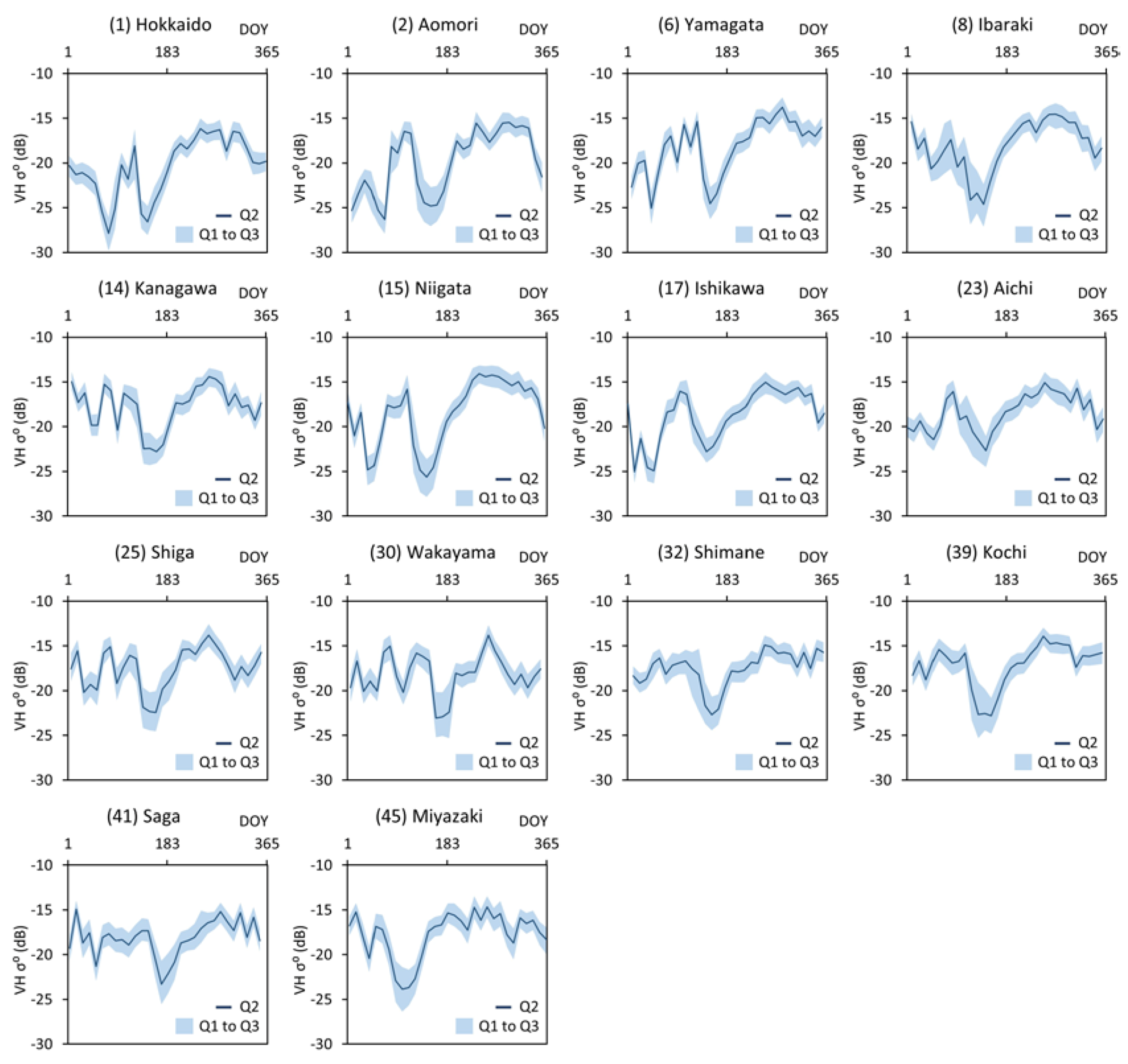
The temporal behavior of Sentinel-1 VH σ0 over each “Paddy” reference field region was analyzed to determine the threshold values for the mask described in 2.5.3. Figure 5 shows the time series of second quartile (Q2) values and the first (Q1) to third (Q3) interquartile range of VH σ0 calculated from 2018 data in each of the 14 “Paddy” reference field regions. In all “Paddy” reference field regions, a local VH σ0 minimum was observed during the irrigated period. Subsequently, VH σ0 increased and reached a peak within a few months. Thereafter, during the latter part of the rice cultivation period, VH σ0 maintained a high value or decreased slightly. Previous studies have shown that VH σ0 decreases during the transplanting period, when the fields are flooded with irrigation water, and then increases during the rice-growing period until around harvest time [23,24,25,26,27,28]. Therefore, rice phenology in broad areas of Japan can be observed in VH σ0 time series. The low VH σ0 values from January to March in Hokkaido, Aomori, Yamagata, Niigata, and Ishikawa prefectures are attributable to snow cover because these prefectures are located in northern Japan, where heavy snow falls in winter.
2.5.3. Masks Used for Provisional Extraction of Paddy Fields
“Forest Area (FA)” mask: A mask for forest area was made based on an updated version of the Hansen Global Forest Change map (v1.6, 2000–2018) [39]. Pixels with a forest area covering more than 30% of the pixel area were specified as forest pixels. On Hansen’s map, forest area is defined by the canopy closure due to vegetation taller than 5 m. The Forest area masking was performed to minimize commission errors in paddy field mapping [17].
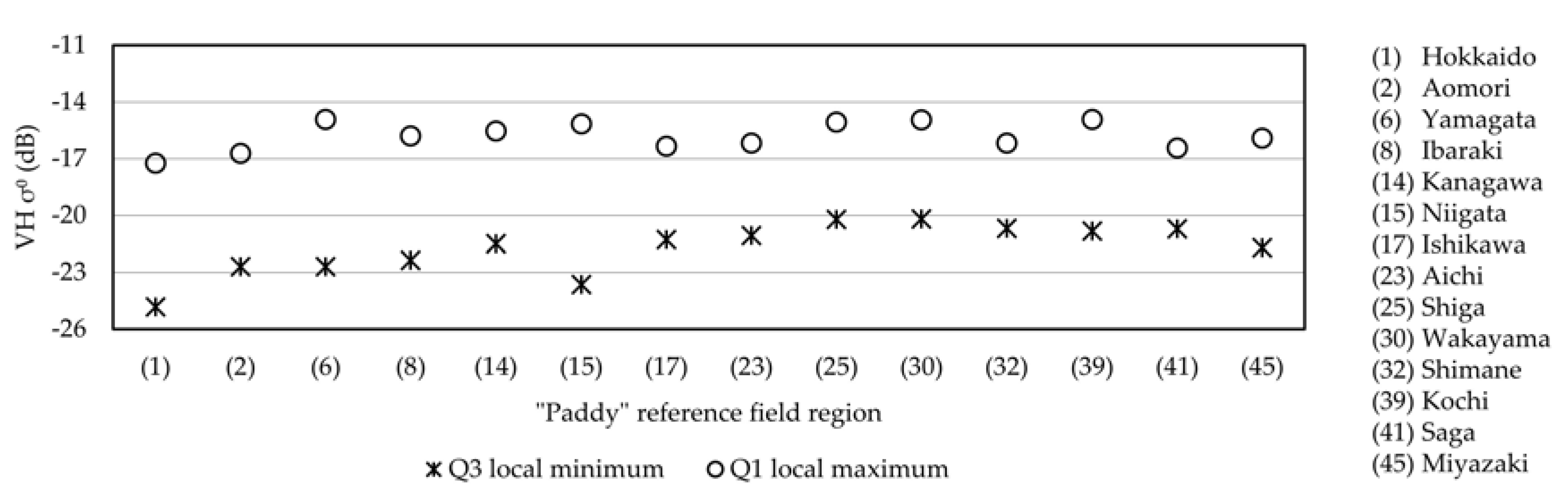
“Local Maximum & Minimum (LMM)” mask: The local maximum σ0 value and the local minimum σ0 value of the Sentinel-1 time series within 90-day moving windows were calculated for each Sentinel-1 image from the period between TS and HE. In this study, the thresholds of the local minimum and local maximum σ0 values were determined by analyzing the temporal behavior of Sentinel-1 VH σ0 values in the “Paddy” reference fields (Figure 5). Figure 6 shows the local minimum Q3 VH σ0 value during the irrigated period and the local maximum Q1 VH σ0 value between the end of the irrigated period and HE for each “Paddy” reference field region. In all “Paddy” field reference regions, the local minimum Q3 VH σ0 value was smaller than −20 dB. The local maximum Q1 VH σ0 value in Hokkaido was slightly below −17 dB, whereas those in other areas were above −17 dB. Therefore, pixels with a local minimum VH σ0 larger than −20 dB or a local maximum VH σ0 smaller than −17 dB, were masked on each Sentinel-1 image. The VH σ0 of paddy fields shows a very distinct minimum when the paddy fields are irrigated just after transplanting and a maximum during the heading stage of the rice plants [26].
“Local Variation (LV)” mask: Local variation values were calculated for each Sentinel-1 image by using the following equation:
local maximum VH σ0 and local minimum VH σ0 are the values calculated for the LMM mask. Pixels with a local variation of less than 5 dB were masked on each Sentinel-1 image. This threshold value, which was also determined by analyzing the temporal behavior of Sentinel-1 VH σ0 values in the “Paddy” reference fields, was selected to differentiate vegetation with clear seasonality from land covers with a constant low or high backscatter such as waterbodies and urban areas [26].
Local variation = Local maximum VH σ0 − Local minimum VH σ0
It should be noted that the FA mask was applied to the entire Sentinel-1 time series, whereas the LMM and LV masks were applied to each Sentinel-1 image composing the Sentinel-1 time series. The pixels of Sentinel-1 images during the irrigated period that were not masked by any of these three masks were extracted as provisional paddy field pixels. In this paper, we refer to the application of this series of three masks as the “S-1” method. We used the S-1 method to prepare a paddy field map of Japan for later comparison with a paddy field map developed by our proposed method.
2.5.4. Mask Based on Sentinel-2 MSI Environmental Indexes
“Sentinel-2 indexes (S2I)” mask: The provisional paddy fields extracted by the S-1 method were reexamined by using water and vegetation indexes, LSWI, NDVI, and EVI, calculated from Sentinel-2 MSI images acquired during the irrigated period. The LSWI is sensitive to the total amount of liquid water in vegetation and its soil background [40], and the NDVI and EVI are sensitive to variations in the vegetation [41,42]. These three indexes were calculated by using Equations (2)–(4), respectively:
where Blue, Red, NIR, and SWIR are the reflectance values at the top of the atmosphere of the B2 band (central wavelength: 490 nm), B4 band (665 nm), B8 band (842 nm), and B11 band (1610 nm) of the Sentinel-2 MSI. Previous studies have revealed that relationships among the LSWI, NDVI, and EVI can be used effectively to extract irrigated areas [9,17,43]. After the three S-1 masks were applied to each Sentinel-1 image, the local maximum “LSWI − NDVI” and “LSWI − EVI” values within the 10 days after the date that the Sentinel-1 image was acquired were calculated, and pixels in which the local maximum “LSWI − NDVI” and “LSWI − EVI” values were both smaller than 0 were masked. These threshold values are based on values proposed by Dong et al. [17]. The pixels of Sentinel-1 images acquired during the irrigated period that were not masked by any of the four masks were extracted as paddy fields. We call the application of this series of four masks the “S-1 & S-2” method in this paper.
2.6. Accuracy Assessment
The accuracy of the paddy field maps was assessed by producer’s accuracy with a pixel-scale resolution of 30 m. The producer’s accuracy indicates the quality of the classification and is calculated by dividing the number of correctly classified reference pixels in each category by the total number of reference pixels in that category [44]. All pixels of the paddy field maps spatially included in the two types of reference field polygons were assessed for accuracy.
3. Results
3.1. Accuracy Assessments in Reference Agricultural Fields
The producer’s accuracy for “Paddy” reference fields was 83.6% by the S-1 method and 79.2% by the S-1 & S-2 method. For “Not paddy” reference fields, the producer’s accuracy was 57.0% by the S-1 method and 92.4% by the S-1 & S-2 method. Thus, the application of the S2I mask following the three S-1 masks caused the producer’s accuracy for “Paddy” reference fields to decrease by 4.4 points and that for “Not paddy” reference fields to increase by 35.4 points.
The producer’s accuracies in each “Paddy” and “Not paddy” reference field region are shown in Table 2 and Table 3, respectively. The producer’s accuracies in “Paddy” reference field regions were 68.6–100.0% by the S-1 method and 68.1–98.3% by the S-1 & S-2 method. The producer’s accuracies in “Not paddy” reference field regions were 29.6–78.4% by the S-1 method and 88.0–97.6% by the S-1 & S-2 method. Thus, the application of the S2I mask decreased the producer’s accuracy in “Paddy” reference field regions by 0–16.3 points and increased the producer’s accuracy in “Not paddy” reference field regions by 14.8–61.1 points.
3.2. Comparison with Existing Paddy Field Maps
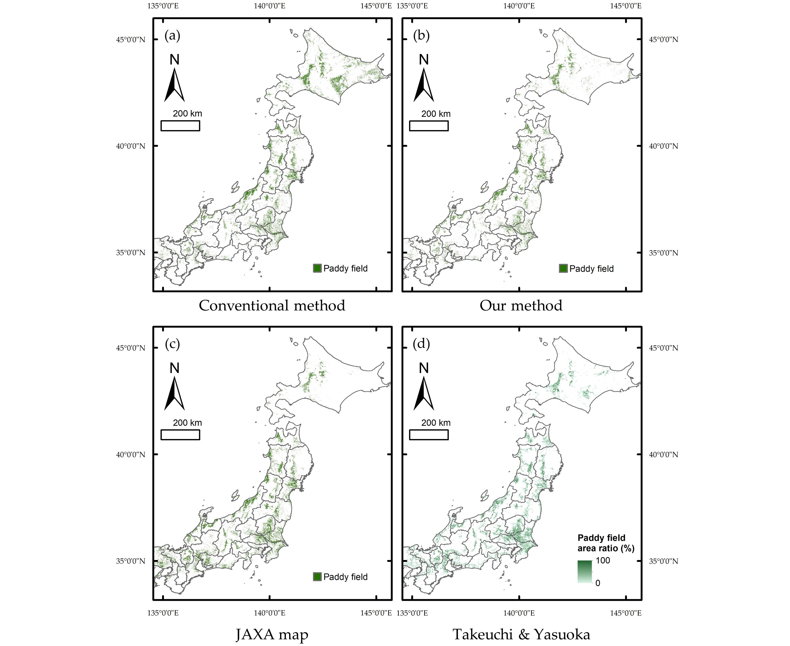
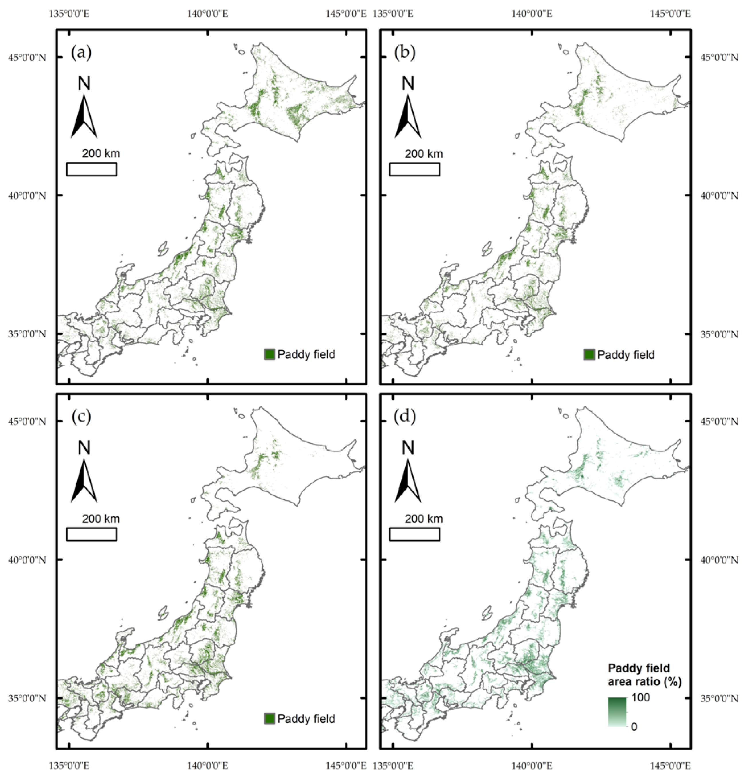
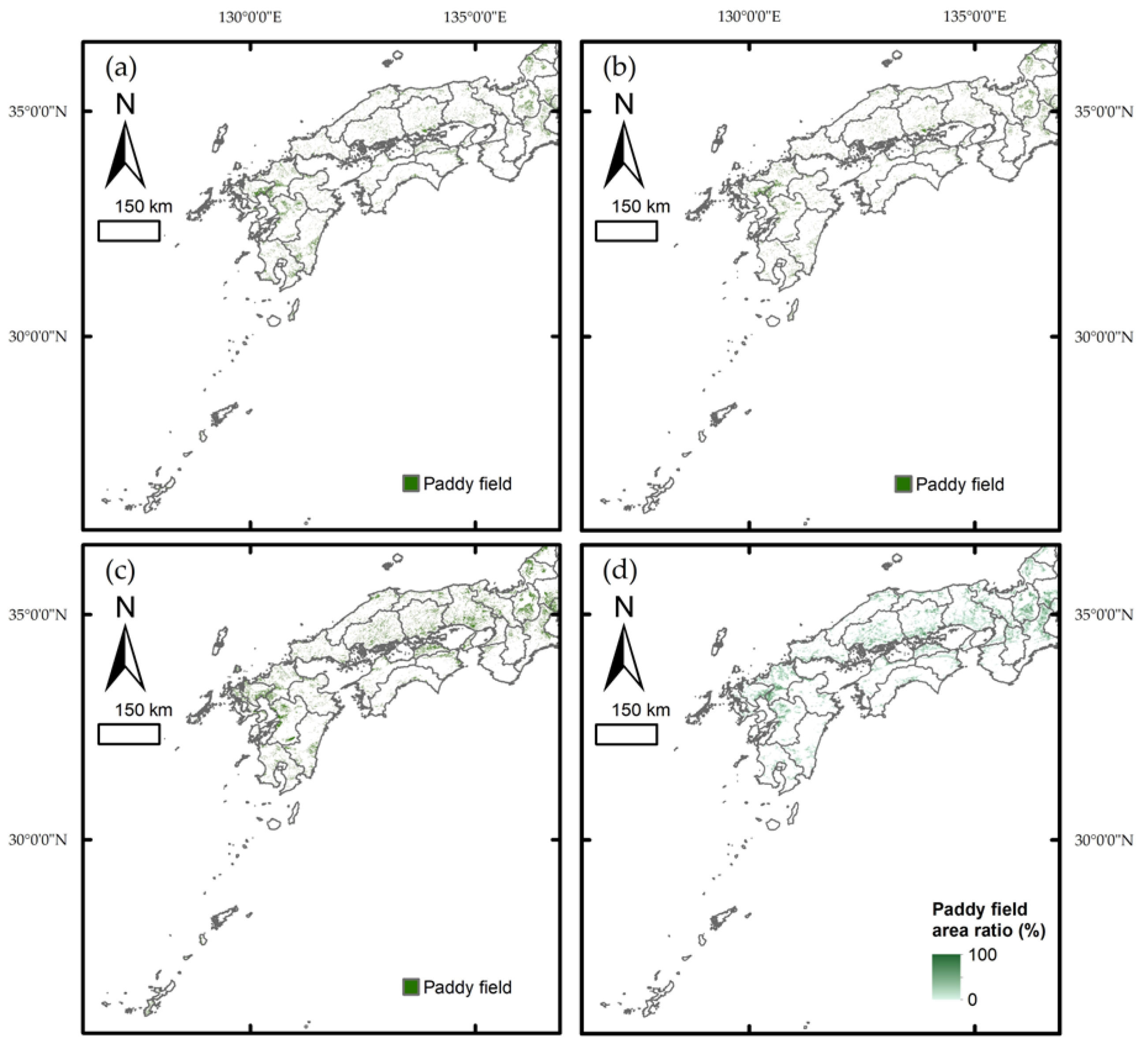
The paddy field maps developed by the S-1 and the S-1 & S-2 methods are compared with the JAXA and TY paddy field maps in Figure 7 and Figure 8. The maps prepared by the S-1 and the S-1 & S-2 methods and the JAXA map have a spatial resolution of 30 m, and the TY map has a 1 km spatial resolution. The paddy field maps developed by the S-1 and the S-1 & S-2 methods have some noticeable characteristics. Compared with the JAXA and TY maps, the map produced by the S-1 method has more paddy field pixels in Hokkaido prefecture. However, the map produced by the S-1 & S-2 method has many fewer paddy field pixels in eastern Hokkaido prefecture. In general, the paddy field distribution in Japan on the maps produced by the S-1 & S-2 method is more similar to the paddy field distributions on the JAXA and TY maps. In eastern Hokkaido, rice is not grown, but non-rice grains are widely grown. Therefore, the application of the S-1 & S-2 method reduces the misclassification of non-paddy fields in that region.
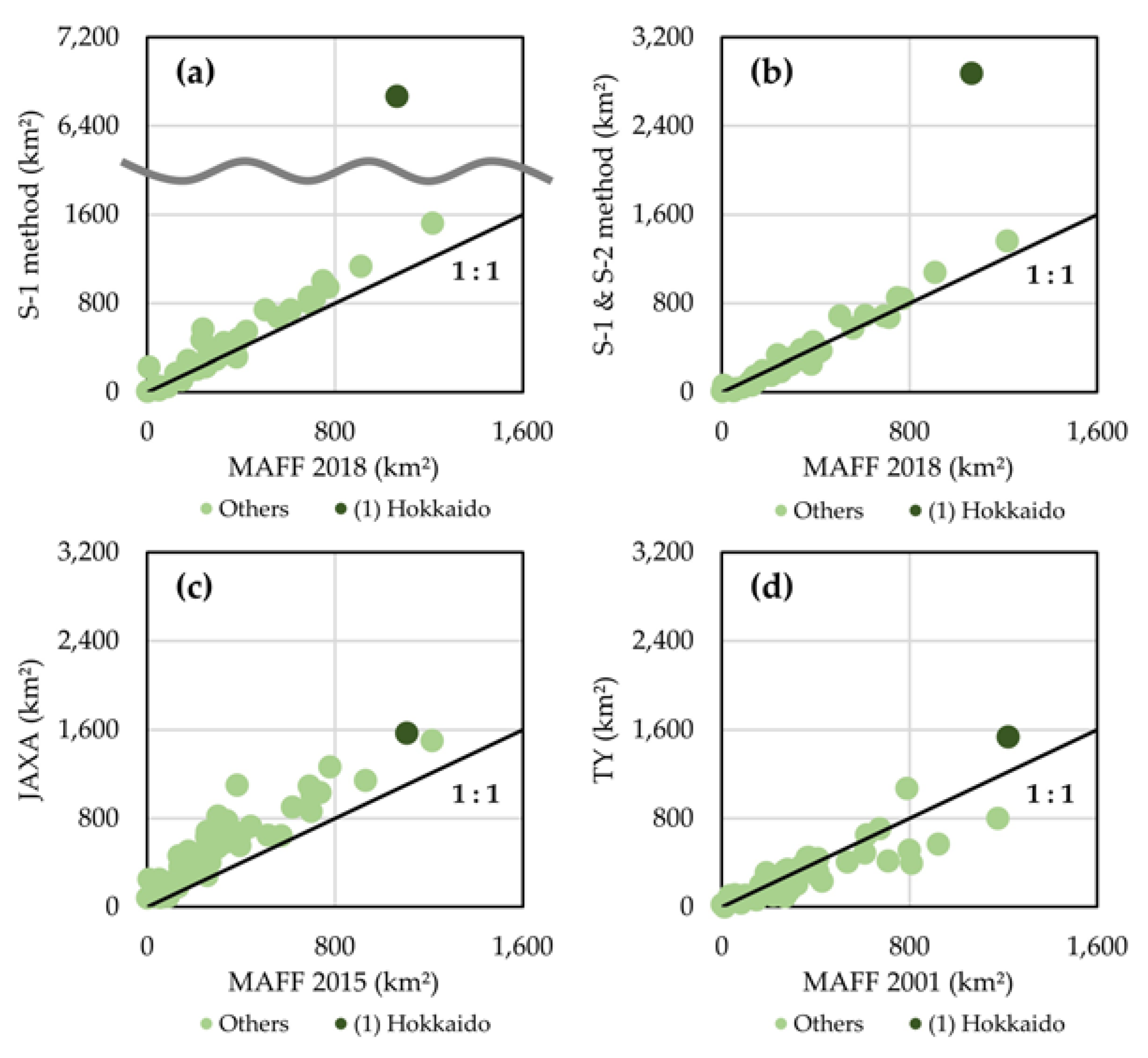
We next compared the paddy field area at the prefecture scale, calculated for each paddy field map, with paddy field area data published by MAFF [32] (Figure 9). When the total paddy field area in Japan according to MAFF was set to 100%, the total paddy field area on the map produced by the S-1 and S-1 & S-2 methods was 156.7% and 112.4%, respectively, and on the JAXA and TY maps, it was 168.5% and 84.7%, respectively. The maps produced by the S-1 and the S-1 & S-2 methods greatly overestimated the paddy field area in Hokkaido prefecture (Figure 9a,b, respectively), but in other prefectures, paddy field areas did not differ significantly from the MAFF values.
To examine the overall trend of paddy field areas on each map relative to the MAFF data, we fitted straight lines to the data shown in Figure 9 by the least-squares method with the y-intercept fixed at 0. Table 4 shows the slopes of the fitted lines together with the coefficients of determination (R²) and the mean square error (MSE) of the map data relative to the MAFF data. The paddy field areas calculated from the maps produced by the S-1 and S-1 & S-2 methods and the JAXA map (slopes > 1) were overestimated compared with the published MAFF areas. In contrast, the paddy field areas on the TY map (slope = 0.86) were underestimated. When Hokkaido was excluded, the areas obtained by the S-1 & S-2 method were still overestimated, but the slope was closer to 1. R² is a measure of how well the areas calculated from each map replicate the MAFF areas at the prefecture scale, where R² = 1 indicates a perfect match between them. For all of Japan, R² values for the S-1 and S-1 & S-2 methods were lower than those for JAXA and TY, whereas when Hokkaido was excluded, R² value for the S-1 & S-2 method was much higher than those for JAXA and TY. MSE is the average of the squared errors between the paddy field area in each prefecture calculated from the paddy field maps and the MAFF areas. When Hokkaido was excluded, MSE values for the S-1 & S-2 method were lower than those of JAXA and TY.
4. Discussion
We proposed a new high-resolution paddy field mapping method that uses Sentinel-1 SAR time series images supplemented by Sentinel-2 optical images. Although some paddy field mapping methods combining SAR and optical images have been proposed previously [19,21,22], those methods used optical images as fundamental data for paddy field extraction; therefore, they could be seriously affected by gaps and biases in the optical images due to cloud cover. In contrast, in our proposed method, the Sentinel-2 images are used only as ancillary data to produce masks based on water and vegetation indexes. As a result, gaps in the Sentinel-2 images did not adversely affect the paddy field mapping accuracy. In this regard, our method is expected to have an advantage for detecting paddy fields at a broad scale.
The producer’s accuracy for “Paddy” reference fields identified by the S-1 & S-2 method was lower than that of fields identified by the S-1 method; this result is reasonable because the additional mask applied to extract paddy fields in the S-1 & S-2 method makes the identification criteria more strict. In contrast, the producer’s accuracy for “Not paddy” reference fields identified by the S-1 & S-2 method was higher compared with the S-1 method. Therefore, to grasp the potential of the S-1 & S-2 method for paddy field mapping, a comprehensive evaluation is needed to account for the decrease of the producer’s accuracy in “Paddy” reference fields and the increase in “Not paddy” reference fields. The map developed by the S-1 & S-2 method has a spatial resolution of 30 m, which is much finer than previous maps based on satellite images with low to medium spatial resolutions. However, this resolution might be still insufficient for validation of the accuracy at the pixel scale for individual agricultural fields in Japan. In 2009, 38% of paddy fields in Japan were smaller than 0.003 km², and 92% of paddy fields were smaller than 0.01 km², according to MAFF [45]. Therefore, we believe that the producer’s accuracy for “Paddy” reference fields (79.2%) identified by the S-1 & S-2 method is still acceptable, and the decrease of 4.4 points in the accuracy for “Paddy” reference fields compared to the S-1 method does not indicate a serious reduction in paddy field extraction accuracy at a broad scale. In contrast, the accuracy for “Not paddy” reference fields of the S-1 & S-2 method was greatly improved, by 35.4 points, compared with that of the S-1 method. This large increase in accuracy justifies the use of the S-1 & S-2 method despite the decrease in accuracy for “Paddy” reference fields. Therefore, we consider the S-1 & S-2 method to be an effective paddy field mapping approach because it reduces the misclassification of non-paddy agricultural fields as paddy fields.
Remarkably, the effectiveness with which the S-1 & S-2 method reduced misclassification differed among regions (Table 4). In particular, in the Koshimizu district, Hokkaido prefecture, 12% of “Not paddy” reference fields were misclassified. The inter-regional variation in accuracy is primarily attributable to gaps in Sentinel-2 images caused by cloud cover. Although unlike previous paddy field mapping methods that use optical images as fundamental data, the S-1 & S-2 method does not generally misclassify or produce no-data pixels because of gaps in the Sentinel-2 images, if there are no cloud-free Sentinel-2 images during the irrigated period, the S2I mask is ineffective. In this situation, therefore, gaps in the Sentinel-2 images can reduce the degree to which the classification accuracy is improved by the S-1 & S-2 method. It is difficult to completely resolve this issue because the effects of cloud cover cannot be controlled, but it should be possible to reduce the uncertainty of the classification by using a larger number of cloud-free optical image scenes. Fortunately, the ESA has planned the launches of Sentinel-2C and Sentinel-2D, and these additional satellites will make it possible to use more Sentinel-2 images in the future. This future increase in the number of Sentinel-2 satellites will reduce the uncertainty of the S-1 & S-2 method by improving its temporal resolution.
This study developed a paddy field map covering a wide area of Japan, except for Hokkaido prefecture, that reproduced well data from MAFF on paddy field areas. The maps produced by the S-1 and S-1 & S-2 methods, however, seriously overestimated the paddy field area in Hokkaido prefecture (Figure 9). This prefecture is in a cooler climate and has more types of agricultural fields covering a larger area (11,450 km²) than the other prefectures; in 2018, the cultivated paddy field area accounted for only 9.3% of the total agricultural field area in Hokkaido prefecture [32]. In contrast, in the other Japanese prefectures, the cultivated paddy field area accounted for 45.4% of the total agricultural field area in 2018 [32]. The maps by JAXA and TY used multi-band optical sensors that are more robust for extracting vegetation type and irrigated agricultural areas in the Hokkaido prefecture than the SAR sensor. One approach to solving the overestimation in Hokkaido prefecture is, as described above, to improve the accuracy of the S2I mask for extracting irrigated areas from satellite images by using a larger number of optical image scenes. Another approach is to refine the threshold values of the LMM and LV masks to improve the accuracy with which paddy fields are extracted from the Sentinel-1 time series data. In this study, we used the same threshold values for these masks to extract paddy fields everywhere in Japan, but the temporal behavior of Sentinel-1 VH σ0 differed greatly among the regions (Figure 5 and Figure 6). Therefore, to further improve the accuracy of paddy field mapping in different regions, appropriate threshold values should be selected for each region instead of using uniform country-scale values. For Japan excluding Hokkaido prefecture, however, the S-1 & S-2 method satisfactorily reproduced MAFF paddy field areas at both country scale and prefecture scale. Therefore, we are convinced that our novel S-1 & S-2 method has a high potential for paddy field mapping in most of Japan, except for the Hokkaido prefecture.
Our efforts in this study are a first step toward providing more accurate paddy field maps wherever paddy rice is grown. Because rice cultivation method and cultivation environments vary greatly from region to region, it is important to confirm whether our method is applicable to mapping paddy fields in other parts of Asia and the world. We examined the new mapping method only in Japan and found that the new method worked well in most of the study area but overestimated in Hokkaido prefecture. This implies that the method can be improved by applying additional masks and thresholds such as a more detailed classification of cultivated crops and land cover types, and by conducting validations over broader and more diverse areas. Here, by using Google Maps Street View, it was relatively easy to select “Paddy” reference fields without on-site visits, but Street View recordings are not always available in every targeted region and time. Furthermore, many paddy fields are likely distributed in areas where few Street View recordings have been made. Therefore, in such regions, it will be necessary to use different approaches for identifying reference fields. Nevertheless, in the future, it would be desirable to expand the target region to regions outside of Japan and to verify the effectiveness of our method after overcoming the issues described above.
5. Conclusions
Through developing paddy field maps for Japan, this study demonstrated the potential of our novel paddy field mapping method using the Sentinel-1 time series supplemented by Sentinel-2 optical images in comparison with the conventional paddy field method using only Sentinel-1 time series data. Furthermore, by comparing our maps with existing paddy field maps and MAFF data on paddy field areas, we evaluated the reproducibility of our paddy field map. Our method, which uses an additional mask based on Sentinel-2 indexes obtained during the irrigated period, shows great potential for reducing the misclassification of non-paddy agricultural fields as paddy fields. The producer’s accuracy for non-paddy reference agricultural fields increased from 57.0% with the conventional method to 92.4% with our proposed method. The paddy field map developed by our proposed method also reproduced well paddy field area data at the prefecture scale more reliably than existing paddy field maps of Japan, except in Hokkaido prefecture where our method systematically overestimated paddy field area. Our advanced method would be extended by covering other land cover types such as cropland, forest, and urban areas, and therefore methodological accuracy can be improved by conducting validations over a wide variety of areas not only in Japan but also in other countries.
Author Contributions
Conceptualization and data collection, S.I. and A.I.; methodology, analysis, validation, and paper writing, S.I.; paper revision, A.I. and C.Y. All authors have read and agreed to the published version of the manuscript.
Funding
This research was funded by the Environment Research and Technology Development Fund (2-1710) of the Ministry of the Environment and the Environmental Restoration and Conservation Agency.
Acknowledgments
We thank the Ministry of the Environment and the Environmental Restoration and Conservation Agency for supporting this work. We thank the Ministry of Agriculture, Forestry and Fisheries for providing the agricultural field polygons. We thank Wataru Takeuchi, University of Tokyo, for approval to use his paddy field map data.
Conflicts of Interest
The authors declare no conflict of interest.
Appendix A
Figure A1.
The 47 prefectures of Japan.

References
- Elert, E. Rice by the numbers: A good grain. Nature 2014, 514, S50–S51. [Google Scholar] [CrossRef] [PubMed] [Green Version]
- Bouman, B.A.M.; Humphreys, E.; Tuong, T.P.; Barker, R. Rice and Water. In Advances in Agronomy; Sparks, D.L., Ed.; Academic Press: Cambridge, MA, USA, 2007; Volume 92, pp. 187–237. [Google Scholar]
- Kiritani, K. Integrated Biodiversity Management in Paddy Fields: Shift of Paradigm from IPM toward IBM. Integr. Pest Manag. Rev. 2000, 5, 175–183. [Google Scholar] [CrossRef]
- Lu, J.; Li, X. Review of rice–fish-farming systems in China—One of the Globally Important Ingenious Agricultural Heritage Systems (GIAHS). Aquaculture 2006, 260, 106–113. [Google Scholar] [CrossRef]
- Stocker, T.F.; Qin, D.; Plattner, G.K.; Tignor, M.; Allen, S.K.; Boschung, J.; Nauels, A.; Xia, Y.; Bex, V.; Midgley, P.M. Climate Change 2013: The Physical Science Basis. In Contribution of Working Group I to the Fifth Assessment Report of the Intergovernmental Panel on Climate Change; IPCC, Cambridge University: Cambridge, MA, USA, 2013; p. 509. [Google Scholar]
- Ito, A.; Tohjima, Y.; Saito, T.; Umezawa, T.; Hajima, T.; Hirata, R.; Saito, M.; Terao, Y. Methane budget of East Asia, 1990–2015: A bottom-up evaluation. Sci. Total Environ. 2019, 676, 40–52. [Google Scholar] [CrossRef] [PubMed]
- LP DAAC—MCD12Q1. Available online: https://lpdaac.usgs.gov/products/mcd12q1v006/ (accessed on 13 May 2020).
- Thenkabail, P.S.; Knox, J.W.; Ozdogan, M.; Gumma, M.K.; Congalton, R.G.; Wu, Z.T.; Milesi, C.; Finkral, A.; Marshall, M.; Mariotto, I.; et al. Assessing future risks to agricultural productivity, water resources and food security: How can remote sensing help? PE&RS Photogramm. Eng. Remote Sens. 2012, 78, 773–782. [Google Scholar]
- Xiao, X.; Boles, S.; Liu, J.; Zhuang, D.; Frolking, S.; Li, C.; Salas, W.; Moore, B. Mapping paddy rice agriculture in southern China using multi-temporal MODIS images. Remote Sens. Environ. 2005, 95, 480–492. [Google Scholar] [CrossRef]
- Xiao, X.; Boles, S.; Frolking, S.; Li, C.; Babu, J.Y.; Salas, W.; Moore, B. Mapping paddy rice agriculture in South and Southeast Asia using multi-temporal MODIS images. Remote Sens. Environ. 2006, 100, 95–113. [Google Scholar] [CrossRef]
- Clauss, K.; Yan, H.; Kuenzer, C. Mapping Paddy Rice in China in 2002, 2005, 2010 and 2014 with MODIS Time Series. Remote Sens. 2016, 8, 434. [Google Scholar] [CrossRef] [Green Version]
- Ozdogan, M.; Gutman, G. A new methodology to map irrigated areas using multi-temporal MODIS and ancillary data: An application example in the continental US. Remote Sens. Environ. 2008, 112, 3520–3537. [Google Scholar] [CrossRef] [Green Version]
- Sun, H.; Huang, J.; Huete, A.R.; Peng, D.; Zhang, F. Mapping paddy rice with multi-date moderate-resolution imaging spectroradiometer (MODIS) data in China. J. Zhejiang Univ.-Sci. A 2009, 10, 1509–1522. [Google Scholar] [CrossRef]
- Zhang, G.; Xiao, X.; Biradar, C.M.; Dong, J.; Qin, Y.; Menarguez, M.A.; Zhou, Y.; Zhang, Y.; Jin, C.; Wang, J.; et al. Spatiotemporal patterns of paddy rice croplands in China and India from 2000 to 2015. Sci. Total Environ. 2017, 579, 82–92. [Google Scholar] [CrossRef] [PubMed]
- Takeuchi, W.; Yasuoka, Y. Mapping of fractional coverage of paddy fields over East Asia using MODIS data. J. Jpn. Soc. Photogramm. Remote Sens. 2004, 43, 20–33. [Google Scholar] [CrossRef]
- Takeuchi, W.; Yasuoka, Y. 11 Subpixel Mapping of Rice Paddy Fields over Asia Using MODIS Time Series. Remote Sens. Glob. Crop. Food Secur. 2009, 2009, 281–296. [Google Scholar]
- Dong, J.; Xiao, X.; Menarguez, M.A.; Zhang, G.; Qin, Y.; Thau, D.; Biradar, C.; Moore, B. Mapping paddy rice planting area in northeastern Asia with Landsat 8 images, phenology-based algorithm and Google Earth Engine. Remote Sens. Environ. 2016, 185, 142–154. [Google Scholar] [CrossRef] [PubMed] [Green Version]
- Xiong, J.; Thenkabail, P.S.; Gumma, M.K.; Teluguntla, P.; Poehnelt, J.; Congalton, R.G.; Yadav, K.; Thau, D. Automated cropland mapping of continental Africa using Google Earth Engine cloud computing. ISPRS J. Photogramm. Remote Sens. 2017, 126, 225–244. [Google Scholar] [CrossRef] [Green Version]
- Zhang, X.; Wu, B.; Ponce-Campos, G.E.; Zhang, M.; Chang, S.; Tian, F. Mapping up-to-Date Paddy Rice Extent at 10 M Resolution in China through the Integration of Optical and Synthetic Aperture Radar Images. Remote Sens. 2018, 10, 1200. [Google Scholar] [CrossRef] [Green Version]
- Gorelick, N.; Hancher, M.; Dixon, M.; Ilyushchenko, S.; Thau, D.; Moore, R. Google Earth Engine: Planetary-scale geospatial analysis for everyone. Remote Sens. Environ. 2017, 202, 18–27. [Google Scholar] [CrossRef]
- Torbick, N.; Chowdhury, D.; Salas, W.; Qi, J. Monitoring Rice Agriculture across Myanmar Using Time Series Sentinel-1 Assisted by Landsat-8 and PALSAR-2. Remote Sens. 2017, 9, 119. [Google Scholar] [CrossRef] [Green Version]
- Onojeghuo, A.O.; Blackburn, G.A.; Wang, Q.; Atkinson, P.M.; Kindred, D.; Miao, Y. Mapping paddy rice fields by applying machine learning algorithms to multi-temporal Sentinel-1A and Landsat data. Int. J. Remote Sens. 2018, 39, 1042–1067. [Google Scholar] [CrossRef] [Green Version]
- Minh, H.V.T.; Avtar, R.; Mohan, G.; Misra, P.; Kurasaki, M. Monitoring and Mapping of Rice Cropping Pattern in Flooding Area in the Vietnamese Mekong Delta Using Sentinel-1A Data: A Case of An Giang Province. ISPRS Int. J. Geo-Inf. 2019, 8, 211. [Google Scholar] [CrossRef] [Green Version]
- Tian, H.; Wu, M.; Wang, L.; Niu, Z. Mapping Early, Middle and Late Rice Extent Using Sentinel-1A and Landsat-8 Data in the Poyang Lake Plain, China. Sensors 2018, 18, 185. [Google Scholar] [CrossRef] [Green Version]
- Nguyen, D.B.; Gruber, A.; Wagner, W. Mapping rice extent and cropping scheme in the Mekong Delta using Sentinel-1A data. Remote Sens. Lett. 2016, 7, 1209–1218. [Google Scholar] [CrossRef]
- Clauss, K.; Ottinger, M.; Kuenzer, C. Mapping rice areas with Sentinel-1 time series and superpixel segmentation. Int. J. Remote Sens. 2018, 39, 1399–1420. [Google Scholar] [CrossRef] [Green Version]
- Bazzi, H.; Baghdadi, N.; El Hajj, M.; Zribi, M.; Minh, D.H.T.; Ndikumana, E.; Courault, D.; Belhouchette, H. Mapping Paddy Rice Using Sentinel-1 SAR Time Series in Camargue, France. Remote Sens. 2019, 11, 887. [Google Scholar] [CrossRef] [Green Version]
- Mandal, D.; Kumar, V.; Bhattacharya, A.; Rao, Y.S.; Siqueira, P.; Bera, S. Sen4Rice: A Processing Chain for Differentiating Early and Late Transplanted Rice Using Time-Series Sentinel-1 SAR Data with Google Earth Engine. IEEE Geosci. Remote Sens. Lett. 2018, 15, 1947–1951. [Google Scholar] [CrossRef]
- Singha, M.; Dong, J.; Zhang, G.; Xiao, X. High resolution paddy rice maps in cloud-prone Bangladesh and Northeast India using Sentinel-1 data. Sci. Data 2019, 6, 1–10. [Google Scholar] [CrossRef]
- Mansaray, L.R.; Huang, W.; Zhang, D.; Huang, J.; Li, J. Mapping Rice Fields in Urban Shanghai, Southeast China, Using Sentinel-1A and Landsat 8 Datasets. Remote Sens. 2017, 9, 257. [Google Scholar] [CrossRef] [Green Version]
- FAOSTAT. Available online: http://www.fao.org/faostat/en/#data/QC (accessed on 13 May 2020).
- E-Stat. Available online: https://www.e-stat.go.jp/stat-search/?page=1 (accessed on 13 May 2020).
- MAFF. Available online: https://www.maff.go.jp/j/study/suito_sakugara/ (accessed on 13 May 2020).
- ESA. Available online: https://earth.esa.int/web/guest/home (accessed on 13 May 2020).
- Li, X.; Zhang, C.; Li, W. Building block level urban land-use information retrieval based on Google Street View images. GIScience Remote Sens. 2017, 54, 819–835. [Google Scholar] [CrossRef]
- Berland, A.; Lange, D.A. Google Street View shows promise for virtual street tree surveys. Urban For. Urban Green. 2017, 21, 11–15. [Google Scholar] [CrossRef]
- Oda, K.; Rupprecht, C.D.D.; Tsuchiya, K.; McGreevy, S.R. Urban Agriculture as a Sustainability Transition Strategy for Shrinking Cities? Land Use Change Trajectory as an Obstacle in Kyoto City, Japan. Sustainability 2018, 10, 1048. [Google Scholar] [CrossRef] [Green Version]
- JAXA ALOS Projects. Available online: https://www.eorc.jaxa.jp/ALOS/lulc/lulc_jindex.htm (accessed on 13 May 2020).
- Hansen, M.C.; Potapov, P.V.; Moore, R.; Hancher, M.; Turubanova, S.A.; Tyukavina, A.; Thau, D.; Stehman, S.V.; Goetz, S.J.; Loveland, T.R.; et al. High-Resolution Global Maps of 21st-Century Forest Cover Change. Science 2013, 342, 850–853. [Google Scholar] [CrossRef] [PubMed] [Green Version]
- Chandrasekar, K.; Sai, M.V.R.S.; Roy, P.S.; Dwevedi, R.S. Land Surface Water Index (LSWI) response to rainfall and NDVI using the MODIS Vegetation Index product. Int. J. Remote Sens. 2010, 31, 3987–4005. [Google Scholar] [CrossRef]
- Carlson, T.N.; Ripley, D.A. On the relation between NDVI, fractional vegetation cover, and leaf area index. Remote Sens. Environ. 1997, 62, 241–252. [Google Scholar] [CrossRef]
- Huete, A.; Didan, K.; Miura, T.; Rodriguez, E.P.; Gao, X.; Ferreira, L.G. Overview of the radiometric and biophysical performance of the MODIS vegetation indices. Remote Sens. Environ. 2002, 83, 195–213. [Google Scholar] [CrossRef]
- Jin, C.; Xiao, X.; Dong, J.; Qin, Y.; Wang, Z. Mapping paddy rice distribution using multi-temporal Landsat imagery in the Sanjiang Plain, northeast China. Front. Earth Sci. 2016, 10, 49–62. [Google Scholar] [CrossRef] [PubMed] [Green Version]
- Story, M.; Congalton, R.G. Accuracy assessment: A user’s perspective. Photogramm. Eng. Remote Sens. 1986, 52, 397–399. [Google Scholar]
- MAFF. Available online: https://www.maff.go.jp/j/wpaper/w_maff/h22_h/trend/part1/chap2/c7_01_05.html (accessed on 13 May 2020).
Figure 1.
Typical dates of rice cultivation in the 47 prefectures of Japan. The day of the year (DOY) of the Transplant Start (TS), Transplant End (TE), and Harvest End (HE) dates was obtained by averaging the dates for 2015–2017 published by MAFF.
Figure 1.
Typical dates of rice cultivation in the 47 prefectures of Japan. The day of the year (DOY) of the Transplant Start (TS), Transplant End (TE), and Harvest End (HE) dates was obtained by averaging the dates for 2015–2017 published by MAFF.

Figure 2.
(a) The 14 prefectures selected as “Paddy” reference field regions; 100 paddy fields from each of the 14 prefectures were selected as “Paddy” reference fields. (b) Six municipal districts in Hokkaido prefecture were selected as regions for “Not paddy” reference fields. All agricultural fields in these six districts were selected as “Not paddy” reference fields.

Figure 3.
Example of a Google Maps Street View of a “Paddy” reference field in Niigata prefecture. (a) and (b) indicate the location of reference paddy fields. Yellow arrows show the view angles of the photographs in (c) and (d) taken from the position indicated by the yellow circle.
Figure 3.
Example of a Google Maps Street View of a “Paddy” reference field in Niigata prefecture. (a) and (b) indicate the location of reference paddy fields. Yellow arrows show the view angles of the photographs in (c) and (d) taken from the position indicated by the yellow circle.

Figure 4.
Flow chart of the two paddy field mapping methods, the conventional method S-1 method and our newly proposed S-1 & S-2 method, and their validation by comparisons with reference fields and existing maps.
Figure 4.
Flow chart of the two paddy field mapping methods, the conventional method S-1 method and our newly proposed S-1 & S-2 method, and their validation by comparisons with reference fields and existing maps.

Figure 5.
Time series variation of Sentinel-1 VH σ0 in 2018 for each “Paddy” reference field region. The first (Q1), second (Q2), and third (Q3) quartiles of VH σ0 over “Paddy” reference fields were calculated for all pixels included within “Paddy” reference fields, with a 10 m spatial resolution. Blue lines indicate the Q2 values, and blue shading indicates the Q1 to Q3 interval.

Figure 6.
The local minimum Q3 value during the irrigated period and the local maximum Q1 value between the end of the irrigated period and HE in each “Paddy” reference field region.
Figure 6.
The local minimum Q3 value during the irrigated period and the local maximum Q1 value between the end of the irrigated period and HE in each “Paddy” reference field region.

Figure 7.
Comparison of paddy field maps of eastern Japan developed in this study with existing maps. Paddy fields in 2018 on the maps developed by the (a) S-1 and (b) S-1 & S-2 methods (30 m spatial resolution). (c) Paddy fields in 2014–2016 on the JAXA map (30 m spatial resolution). (d) Paddy fields in the early 2000s on the TY map (1 km spatial resolution).

Figure 8.
Comparison of paddy field maps of western Japan developed in this study with the existing maps. Paddy fields in 2018 on the maps developed by the (a) S-1 and (b) S-1 & S-2 methods (30 m spatial resolution). (c) Paddy fields in 2014–2016 on the JAXA map (30 m spatial resolution). (d) Paddy fields in the early 2000s on the TY map (1 km spatial resolution).

Figure 9.
Comparisons of paddy field areas in each prefecture calculated from each paddy field map with paddy field areas published by MAFF: (a) S-1 method and (b) S-1 & S-2 method versus 2018 MAFF data for both food rice and feed rice. (c) JAXA versus 2015 MAFF data for both food rice and feed rice. (d) TY versus 2001 MAFF data for food rice.

Table 1.
Characteristics of the satellite data used in this study.
| Sensor | Provider | Band | Resolution | Wavelength | Use | |
|---|---|---|---|---|---|---|
| Satellite data | Sentinel-1 SAR | ESA | C (VH) | 10 m | Interferometric Wide Mode | |
| Sentinel-2 MSI | ESA | B2 | 10 m | 490 nm | Blue | |
| B4 | 10 m | 665 nm | Red | |||
| B8 | 10 m | 842 nm | Near-infrared | |||
| B11 | 20 m | 1610 nm | Short-wave infrared 1 |
Table 2.
Producer’s accuracies in each of the 14 “Paddy” reference field regions (30 m pixel-scale resolution). See Figure 2a for reference field region locations.
Table 2.
Producer’s accuracies in each of the 14 “Paddy” reference field regions (30 m pixel-scale resolution). See Figure 2a for reference field region locations.
| Method | (1) | (2) | (6) | (8) | (14) | (15) | (17) |
|---|---|---|---|---|---|---|---|
| Hokkaido | Aomori | Yamagata | Ibaraki | Kanagawa | Niigata | Ishikawa | |
| S-1 | 81.7% | 84.5% | 86.6% | 92.9% | 98.2% | 100.0% | 70.9% |
| S-1& S-2 | 77.1% | 84.5% | 79.2% | 91.1% | 98.2% | 98.3% | 70.9% |
| Method | (23) | (25) | (30) | (32) | (39) | (41) | (45) |
| Aichi | Shiga | Wakayama | Shimane | Kochi | Saga | Miyazaki | |
| S-1 | 68.6% | 77.4% | 76.1% | 84.9% | 82.3% | 75.3% | 91.1% |
| S-1& S-2 | 68.1% | 74.8% | 70.3% | 76.1% | 79.5% | 70.3% | 74.8% |
Table 3.
Producer’s accuracies in each of the six “Not paddy” reference field regions in Hokkaido prefecture (30 m pixel-scale resolution). See Figure 2b for reference field region locations.
Table 3.
Producer’s accuracies in each of the six “Not paddy” reference field regions in Hokkaido prefecture (30 m pixel-scale resolution). See Figure 2b for reference field region locations.
| Method | (a) | (b) | (c) | (d) | (e) | (f) |
|---|---|---|---|---|---|---|
| Obihiro | Shihoro | Shibecha | Betsukai | Kiyosato | Koshimizu | |
| S-1 | 47.5% | 78.4% | 71.6% | 29.6% | 64.8% | 58.4% |
| S-1& S-2 | 97.1% | 93.2% | 94.9% | 90.7% | 97.6% | 88.0% |
Table 4.
Slopes of straight lines fitted to the relationships shown in Figure 9 with the y-intercept fixed at 0, together with the coefficients of determination (R²) and the mean square errors (MSE) relative to the MAFF data.
Table 4.
Slopes of straight lines fitted to the relationships shown in Figure 9 with the y-intercept fixed at 0, together with the coefficients of determination (R²) and the mean square errors (MSE) relative to the MAFF data.
| All of Japan | Excluding Hokkaido | ||||
|---|---|---|---|---|---|
| S-1 | S-1 & S-2 | JAXA | TY | S-1 & S-2 | |
| Slope | 1.87 | 1.26 | 1.50 | 0.86 | 1.06 |
| R2 | 1.87 | 1.26 | 1.50 | 0.86 | 1.06 |
| MSE (km2 × km2) | 682,924 | 73,513 | 77,310 | 23,474 | 3894 |
© 2020 by the authors. Licensee MDPI, Basel, Switzerland. This article is an open access article distributed under the terms and conditions of the Creative Commons Attribution (CC BY) license (http://creativecommons.org/licenses/by/4.0/).
Share and Cite
MDPI and ACS Style
Inoue, S.; Ito, A.; Yonezawa, C. Mapping Paddy Fields in Japan by Using a Sentinel-1 SAR Time Series Supplemented by Sentinel-2 Images on Google Earth Engine. Remote Sens. 2020, 12, 1622. https://doi.org/10.3390/rs12101622
AMA Style
Inoue S, Ito A, Yonezawa C. Mapping Paddy Fields in Japan by Using a Sentinel-1 SAR Time Series Supplemented by Sentinel-2 Images on Google Earth Engine. Remote Sensing. 2020; 12(10):1622. https://doi.org/10.3390/rs12101622
Chicago/Turabian StyleInoue, Shimpei, Akihiko Ito, and Chinatsu Yonezawa. 2020. "Mapping Paddy Fields in Japan by Using a Sentinel-1 SAR Time Series Supplemented by Sentinel-2 Images on Google Earth Engine" Remote Sensing 12, no. 10: 1622. https://doi.org/10.3390/rs12101622
Note that from the first issue of 2016, this journal uses article numbers instead of page numbers. See further details here.